Abstract
Climate parameter projections obtained by global and regional models (GCM and RCM, respectively) offer a challenge to many researchers in terms of controlling the quality of the outcome data using several scales. In the literature, the proposed models, namely statistical downscaled and regression-based models, are mostly used to adjust the RCM data series. Contrariwise, in practice, these conceptual models perform poorly in certain cases and at certain scales. In this regard, a new downscaling model is proposed herein for annual rainfall projection, based on fusion models, namely polynomial regression (Poly_R), classification and regression tree (CRT), and principal component regression (PCR). The proposed model downscales the rainfall data projected by the coupled model intercomparison phase five (CMIP5) under different representative concentration pathway (RCP) scenarios (2.6, 4.5, 6.0, and 8.5) using overlapping data between the observation and the CMIP5 historical data. This process aims to define the framework for how to use the output equations and algorithm to correct data forecasting by RCM. Generally, the model can be summarized into three levels of analysis, starting with an iterative downscaling using a trendline model that is obtained by Poly_R fitting. Then, the CRT is used to classify and predict the data in subsets. Finally, multiple regression is given by a PCR model using principal components and standardized variables. The final model is also used to downscale the predicted data obtained by both previous models. The results provide the best performance of the fusion model in all RCP cases, compared to the delta change correction and linear scale models. This performance is proved by R2 scores which range between 0.87 and 0.95.
1. Introduction
Evaluating hydroclimatic indices under future climate change conditions is crucial for informing decision-makers about future water availability. This information must also be considered in future plans for civil construction and development [1,2]. Future studies on rainfall variability often use data from global climate models (GCMs), which explore the causes of climate change and the relationship between natural climate variability and human activities. GCMs are widely used in climate research to study global and regional climate patterns, assess the potential impacts of climate change, and evaluate the effectiveness of different mitigation and adaptation strategies. Unfortunately, GCMs have a very low spatial resolution, which can lead to limitations in accurately representing local climate characteristics [3]. In order to address these limitations, researchers often use certain techniques such as downscaling, which involves refining the GCM outputs to a finer scale to better represent local conditions.
Downscaling can be performed using statistical methods or by using regional climate models (RCM) that possess a higher spatial resolution. Generally, the RCM model uses incorporating topography, land–sea contrast, surface heterogeneities, and certain information about physical processes using a spatial resolution from 20 to 50 km [4]. The statistical downscaling (SD) method is based on historical observed data to create an empirical relationship between the GCM and observed data [5,6]. The most commonly used SD methods are regression-based [7,8,9] and correction-based equations [10].
Artificial neural networks (ANNs) offer another regression-based method, which is able to capture non-linear relationships, and these networks tend to perform better than the multiple linear regression method in certain cases [11]. ANNs also yield physically interpretable linkages to surface climate. However, ANN models require large time series data and are incapable of predicting values outside of the historical dataset [4].
This work aims to propose a new model to downscale the annual rainfall data projected by the coupled model intercomparison phase five (CMIP5) using representative concentration pathway (RCP) scenarios, such as RCP 2.6, RCP 4.5, RCP 6.0, and RCP 8.0 [12]. The idea is to fuse two different results obtained by polynomial and tree-regression (Poly_R and CRT, respectively) methods using principal components regression (PCR). In general, the new model follows three steps of processing using overlapping data series of observed and simulated historical data. The Trentino-Alto Adige region (in northern Italy) has been selected in our study due to the significant temporal variability of annual rainfall observed there during the 17 years under study, as well as for the high diversity of elevation which characterizes this region.
In the experimental part, the new method shows in detail its efficiency in correcting the large errors between CMIP5 and real data, followed by a comparative study to explain its performance compared to other models mostly used in the state of art. This technique provides an improvement when applying consecutive processing on a downscaled output using different classifications by CRT and PCR models.
2. Related Work
In the literature, several statistical methods are based on regression techniques using linear and machine-learning models to correct future RCM multiscale data. Generally, these models use historical observed and RCM data to define a new factor or equation for climate downscaling in each specific region. Examples of these methods are those implemented by the soil and water assessment tool (SWAT) [13], which are the linear scaling (LS) model and delta change correction (DCC) model.
2.1. Linear Scaling Model
The LS model is one of the statistical methods applied to downscale the rainfall and temperature projection data obtained by RCM, based on the change factors α and β, respectively [14]. Both factors are obtained by dividing the overlapping data of real observation on the data projection, as is shown by Equations (1) and (2), respectively. Using these factors allows to correct the future RCM rainfall and temperature data.
where and are the future rainfall and temperature downscaled data, respectively; and are the future rainfall and temperature data projection by RCM, respectively; and are the historical rainfall and temperature real data, respectively; and and are the historical rainfall and temperature data projection, respectively.
2.2. Delta Change Correction Model
This method uses the extreme rainfall or temperature values (PE or TE, respectively) obtained during T years by the generalized extreme value distribution model (GEV). The extreme values are used to determine the correction factor to downscale RCM future data using the following functions [15]:
where and are the future rainfall and temperature downscaled data, respectively; and are the future rainfall and temperature data projection by RCM, respectively; and are the extreme rainfall and temperature real data, respectively; and and are the extreme rainfall and temperature data projection, respectively.
3. Material and Methods
In this part, the used methods, the study area, and the newly proposed data-driven downscaling model are detailed. This is used to adjust the CMIP5 annual rainfall projections given by RCM, under different scenarios, as detailed in the following sub-sections.
3.1. Used Method
3.1.1. Polynomial regression
Polynomial regression (Ploy_R) is a case of a multiple non-linear regression model with only one independent variable (X). In this function, we regress the variable X on powers () [16], as follows:
3.1.2. Classification Regression Tree
The tree-driven regression algorithm is one of the family of machine-learning models. In this regard, four models were developed using the tree technique, including a classification and regression tree (CRT), random forest (RF), gradient-boosting decision tree (GBDT), and extreme gradient boosting (XGB) [17]. CRT and RF belong to supervised learning. In time series analysis, both models provide a stable performance for data downscaling under different scales [18].
3.1.3. Principal Component Regression
Generally, this model performs better than a simple regression. It is based on data classification and regression of each subset using principal components (). This method regresses the independent variable () using a standardized variable () and principal component () [19], as follows:
3.2. Metrics of Performance
A set of statistical parameters has been applied in the experimental part of this paper to control the quality of performance provided by each sub-model used in this proposal. These metrics are the coefficient of determination (R2), adjusted coefficient of determination (R2Adj), root mean square error (RMSE), and residual analysis [20,21,22]. These were applied to compare the predicted values with the observed values.
4. Study Area and Data
Trentino-Alto Adige is located in the northern part of Italy. It has an approximate total surface area of 13,612 km2 and a demography of 523,000 people. Alto Adige is located between a latitude of 45.67° N and 47.10° N, and a longitude of 10.37° E and 12.48° E. The region is well known for its diverse geography, which includes the towering Dolomite Mountains and rolling hills dotted with vineyards and apple orchards. The climate in Alto Adige is continental, with warm summers and cold winters. The average maximum temperature in the summer months, especially during July and August, is around 25 °C, while the average minimum temperature in the winter months is around −5 °C. The region experiences an average amount of annual rainfall of around 895 mm. This region is characterized by diverse elevations ranging from 200 m to 4565 m, which are distributed relatively from the central to the northern part of the region, between an urban and a mountainous area, respectively [23]. The maximum altitude in the Trentino-Alto Adige region is more observed in the western part between 2295 m and 4565 m (Figure 1). In this work, the annual rainfall historical data of the Trentino-Alto Adige region observed by the monitoring station between 2005 and 2022 are presented as the response variable for the proposed model. On the other side, the CMIP5 data projection for the same region is obtained by the RCM according to a multi-model ensemble under different RCPs scenarios, which are 2.6, 4.5, 6.0, and 8.5. The CMIP5 data are supported by the IPCC’s fifth assessment report, which is available on the climate knowledge portal website of the World Bank Group: https://climateknowledgeportal.worldbank.org/country/italy/cmip5 (accessed on 20 January 2023).
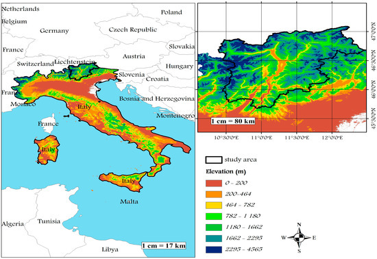
Figure 1.
Map of the Trentino-Alto Adige region showing the spatial elevations and its regional location in Italy.
Figure 2 shows quantitative and qualitative statistical tools to describe the data variability and distribution of each dataset used in the experimental part of this paper. This part gives information about a comparative analysis between the CMIP5 data series under each scenario and the observed data, using the histogram of density, the curve of the values compared to the mean, and the quantile values (first quantile, median, and third quantile). According to real observations that were obtained by the Trentino-Alto Adige meteorological station, the region underwent a humid period between 2005 and 2015, where the annual rainfall exceeded an average of 958.20 mm. In 2009 and 2010, the rainfall accumulation reached the maximum value during this period. However, between 2016 and 2022, a drought phase was observed in the region, while the minimum extreme value is 920 mm. This was observed during 2019 and 2022 (Figure 2(B1)). Generally, the rainfall pattern in the Trentino-Alto Adige region is non-stationary, demonstrated in Figure 2(C1) by a median value above the average with a variability equal to 0.031. All cases where rainfall data were projected by the RCM under RCP scenarios exhibit a high diversity in rainfall variability and distribution (Table S1). According to Scenario 2.6, the rainfall data follow the Weibull distribution during the whole period (Figure 2(B2)), followed by a periodic variability between wet and dry; during the periods of 2005–2008 and 2013–2019, the region exhibited two phases of humidity, demonstrated by a maximum rainfall value equal to 970 mm which was observed in 2016.
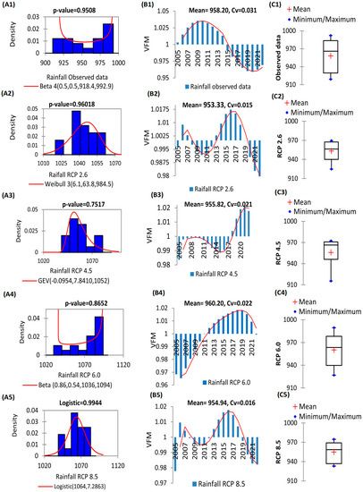
Figure 2.
Statistical description of observed and projected annual rainfall data in the Trentino-Alto Adige region using RCP scenarios, given by density curve (A), histograms of values from the mean (B), and boxplots (C). CV: coefficient of variation.
In addition, during the time range of 2009–2012 and 2020–2022, a drought was observed in this region (Figure 2(B2)), which reached a minimum value of 920 mm (Figure 2(C2)). The data projected by the RCP 2.6 scenario provide a large gap when compared with the actual observation. Contrariwise, the RCP 4.5 rainfall data have a symmetric variability compared to the real observation, in which the series started with a dryness phase between 2005 and 2017. Then, a period of humidity was observed between 2018 and 2022, in which the rainfall showed a maximum value of 980 mm in 2021. During this period, the projected data follow a GEV distribution (Figure 2(C1)). Moreover, the data obtained under RCP 6.0 have the same distribution as the previous projection. The average value of this series is close to the mean actual data. Generally, this series is the best which provides a near variability to actual data (Table S1). The only difference is the temporal data distribution where the data have a symmetric distribution compared to actual observation (Figure 2(B1–B5)). The data obtained by the RCP 8.5 scenario also exhibit similarity with downscaled data under the 4.5 scenario, where the variability of both series is very close, demonstrated by a CV equal to 0.16 and 0.15, respectively.
5. Experimental Part
In this section, the model proposed to downscale CMIP5 rainfall data projection, obtained under different RCP scenarios, is represented in Figure 3. A flowchart summarizes in detail the three fundamental analyses step by step. The model process is a form of framework used to increase the quality of the input data. The observed data histories measured by the meteorological station are used firstly as the response variable of the downscaling model and secondly to control the performance of the outcome, while the overlapping data simulated by the RCM are selected in the first and second steps as the independent variable (Xi) of each sub-model.
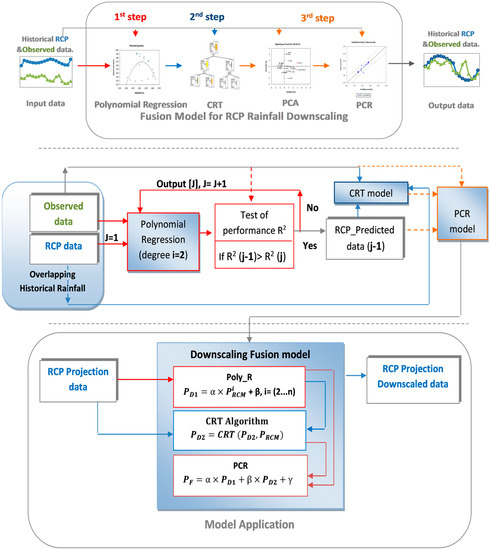
Figure 3.
Flowchart summarizes the fusion model steps proposed for CMIP5 annual rainfall downscaling. R2: coefficient of determination; j: number of iterations. PD1, PD2, and PF are the downscaled data by each sub-model. Poly_R: polynomial regression; PCA: principal component analysis; PCR: principal component regression; CRT: classification and regression tree.
The proposed model starts the procedure of data correction by using a non-linear adjustment between the real and simulated data for each RCP scenario to define the trend equation that will be applied for CMIP5 data downscaling (Table S2). The polynomial method produces a good response to rainfall data distribution. However, the model parameters vary from one scenario to another. For this reason, we have defined an iterative process by this method using the second degree of power. In the first iteration, the sub-model uses the projection data of each scenario as univariate. Then, a validation test will be applied to the predicted data using the R2 to verify how the data fit with the real observation. The procedure iteratively uses the outcome results as input for the next step (Table S2). The downscale analysis stops when the R2 of iteration (j) shows a value lower than the one obtained in iteration (j-1).
According to Figure 4, the application of the second degree of the polynomial model in two iterations gives a good fit, provided by an R2 ranging between 0.52 and 0.61. On the other side, during the first iteration of applying Poly_R, the results show a good fit of 0.69 (Figure 4(A3)).
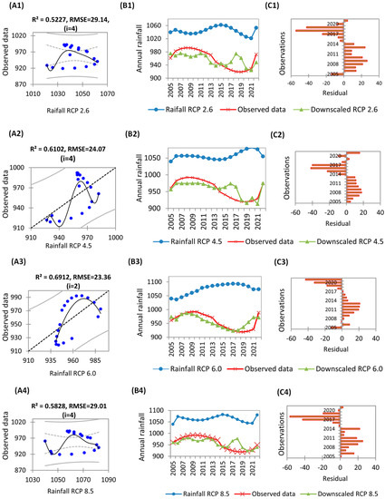
Figure 4.
Non-linear regression scutter graphs (A,B) followed by residual histograms (C) to compare actual and RCP rainfall downscaling obtained by the Poly_R function. R2: coefficient of determination; RMSE: root mean square error.
According to the graphs shown in Figure 4(B1–B4), a significant improvement is observed by the predicted data when compared with the CMIP5 data projected by the four scenarios. In the second step, the proposed model uses a multivariate classification via the application of CRT to the data predicted by the Poly_R model and projected by the RCP scenario as an independent variable of the CRT model. This classification helps to provide satisfactory results of data downscaling compared to the previous model. According to Figure 5(A1–A4), a good fit is observed between the actual data and the predicted series by the CRT model, which is demonstrated by an R2 equal between 0.6194 and 0.8019.
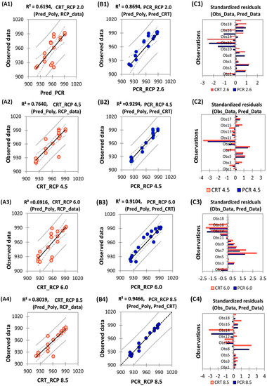
Figure 5.
Regression scutter graph (A,B) and histogram of the residuals (C) between the actual and downscaled rainfall obtained by the CRT and PCR models. R2: coefficient of determination.
In all scenarios, an improvement of the downscaled model was observed when comparing results to the first step of data correction. The application of the RCP model to downscale CMIP5 data by using the results obtained by both correction models (Poly_R and CRT) shows very good results. The PCR classifies the outcome data obtained by the previous models into clusters to estimate the standardized variable. This step helps to provide a very good estimation, which is proved by an R2 ranging between 0.894 and 0.9466. The regression plots and the residual analysis show that the PCR model exhibits the best performance and provides a good response in all RCP scenarios, where the adjustment values fall within the confidence interval better than the CRT outcome. As a result, the fusion model produces a set of equations that will be used to downscale the CMIP5 rainfall data forecasting in the application phase.
6. Validation and Performance
The performance and the validity of the proposed model are provided in this section by comparing the outcome results for each RCP scenario with predicted data obtained by LS and DCC downscaling models. Both models were applied using the SWAT software.
We used statistics metrics including R2, R2Adj, and RMSE to control the performance and the error tendency given by each model. A graphical representation for the whole predicted rainfall series is also given to monitor and compare in detail the downscaled values with the real one during the time period. In this part, the performance analysis applied to the CMIP5 data assessment under all RCP scenarios (2.6, 4.5, 6.0, and 8.5) is well explained in Figure 6.
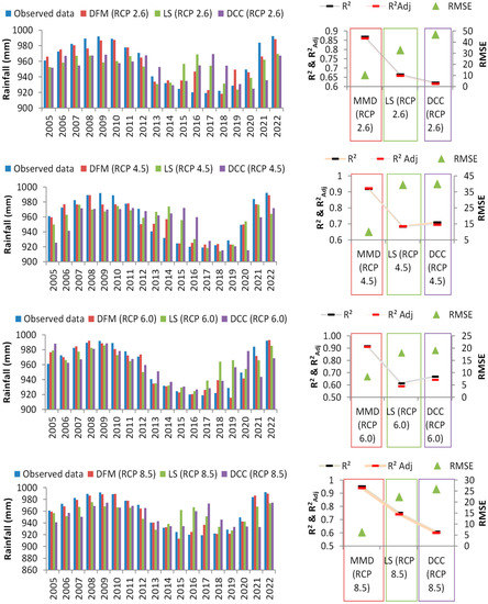
Figure 6.
Histograms of actual and downscaled annual rainfall data obtained by the proposed downscaling fusion model (DFM) compared with LS and DCC downscaled models of SWAT, followed by statistical performance. R2: coefficient of determination; R2Adj: adjusted coefficient of determination; RMSE: root mean square error.
The results show a very good performance of the proposed model with all projected rainfall data series, given by an R2Adj between 0.87 and 0.94. The model provides very low errors of RMSE, which vary between 5 mm to 10 mm. On the other hand, the LS model performs better than the DCC model when using data series obtained under the RCP 2.6 and 8.5 scenarios. However, with the data provided by the RCP 4.5 and 6.0 scenarios, the LS model produces fewer errors than the DCC downscaling model in each case of data processing. The histogram of the downscaled rainfall projection versus actual observation shows that the new model provides the best estimation between 2005 and 2022. When using rainfall data simulated under the 2.6 and 4.5 scenarios, the models gave only one underestimated value each which were observed in 2016 and 2014, respectively. On the other hand, the proposed model showed 2/14 underestimations of data when processing the data series obtained under the RCP 6.0 and RCP 8.5 scenarios. This bias estimation was observed in 2005 and 2018, respectively.
7. Conclusions and Summary
Climate change significantly impacts future biodiversity and the ecosystem. Good knowledge of several natural phenomena is based mainly on the good quality of the climate data projected by GCM and RCM. This work aims to propose a new method to downscale the CMIP5 rainfall data, under different RCP scenarios.
The new proposition is a fusion of three sub-models of the machine-learning family, which were applied to annual rainfall data observed in the Trentino-Alto Adige region between 2005 and 2022.
The first step was to iteratively apply a Poly_R model of a second-degree power on the rainfall simulated data by each scenario. A performance of 0.69 was observed after the first iteration of adjusting projected data by the Poly_R model. Then, improvements of RCP 2.6, 4.5, and 8.5 data downscaling by the Poly_R model were remarked in the second iteration, where the R2 equaled between 0.52 and 0.62. The CRT model which was applied to the outcome data obtained by the previous model showed a good adjustment between 0.60 and 0.80. This performance was more noticeable when using rainfall data under RCP 4.5 and 8.5. Moreover, the application of the PCR model to downscaling data provided by both previous sub-models gave the best performance, which was proven by an R2 between 0.86 and 0.94. The quality of the performance was also approved and compared against the LS and DCC models, where the proposed model proved the most efficient assessment in all RCP scenarios.
The good performance of this method using different scenarios shows its capacity for multiscale application. The method does not depend on the region of study because no physical parameters were used as input variables. This technique can also be employed to correct the estimation biases of several models in the hydro climatological field.
Supplementary Materials
The following supporting information can be downloaded at: https://www.mdpi.com/article/10.3390/engproc2023039055/s1, Table S1: Statistic of observed and CMIP5 projected rainfall data in Trentino-Alto Adige under different RCP scenarios; Table S2: Performance analysis of polynomial regression model to downscale CMIP5 annual rainfall data projection using different iterations, followed by model’s equation.
Author Contributions
All authors of this manuscript have directly participated in this study. A.A. worked on data collection, statistical analysis, modeling, validation, and comparison. A.L. worked on the research method, supervision, co-editing, and reviewing. I.K. worked on mapping. All authors have read and agreed to the published version of the manuscript.
Funding
This research received no external funding.
Institutional Review Board Statement
Not applicable.
Informed Consent Statement
Not applicable.
Data Availability Statement
The data presented in this study can be requested from the corresponding author. They are also available in the Climate Change Knowledge Portal, https://climateknowledgeportal.worldbank.org/country/italy/cmip5 (accessed on 20 January 2023).
Acknowledgments
We wish to thank the Free University of Bozen-Bolzano, Italy, for providing advice and feedback.
Conflicts of Interest
The authors declare no conflict of interest.
References
- Sachindra, D.; Ahmed, K.; Rashid, M.; Shahid, S.; Perera, B. Statistical downscaling of precipitation using machine learning techniques. Atmos. Res. 2018, 212, 240–258. [Google Scholar] [CrossRef]
- Noor, M.; Ismail, T.; Chung, E.-S.; Shahid, S.; Sung, J.H. Uncertainty in Rainfall Intensity Duration Frequency Curves of Peninsular Malaysia under Changing Climate Scenarios. Water 2018, 10, 1750. [Google Scholar] [CrossRef]
- Onyutha, C.; Tabari, H.; Rutkowska, A.; Nyeko-Ogiramoi, P.; Willems, P. Comparison of different statistical downscaling methods for climate change rainfall projections over the Lake Victoria basin considering CMIP3 and CMIP5. J. Hydro-Environ. Res. 2016, 12, 31–45. [Google Scholar] [CrossRef]
- Trzaska, S.; Schnarr, E. A Review of Downscaling Methods for Climate Change Projections; United States Agency for International Development by Tetra Tech ARD: Washington, DC, USA, 2014; pp. 1–42. [Google Scholar]
- Liu, D.L.; Zuo, H. Statistical downscaling of daily climate variables for climate change impact assessment over New South Wales, Australia. Clim. Chang. 2012, 115, 629–666. [Google Scholar] [CrossRef]
- Busuioc, A.; Chen, D.; Hellström, C. Performance of statistical downscaling models in GCM validation and regional climate change estimates: Application for Swedish precipitation. Int. J. Clim. 2001, 21, 557–578. [Google Scholar] [CrossRef]
- Hessami, M.; Gachon, P.; Ouarda, T.B.; St-Hilaire, A. Automated regression-based statistical downscaling tool. Environ. Model. Softw. 2008, 23, 813–834. [Google Scholar] [CrossRef]
- Bürger, G.; Chen, Y. Regression-based downscaling of spatial variability for hydrologic applications. J. Hydrol. 2005, 311, 299–317. [Google Scholar] [CrossRef]
- Chen, J.; Brissette, F.P.; Leconte, R. Assessing regression-based statistical approaches for downscaling precipitation over North America. Hydrol. Process. 2013, 28, 3482–3504. [Google Scholar] [CrossRef]
- Mami, A.; Raimonet, M.; Yebdri, D.; Sauvage, S.; Zettam, A.; Perez, J.M.S. Future climatic and hydrologic changes estimated by bias-adjusted regional climate model outputs of the Cordex-Africa project: Case of the Tafna basin (North-Western Africa). Int. J. Glob. Warm. 2021, 23, 58–90. [Google Scholar] [CrossRef]
- Vu, M.T.; Aribarg, T.; Supratid, S.; Raghavan, S.V.; Liong, S.-Y. Statistical downscaling rainfall using artificial neural network: Significantly wetter Bangkok? Theor. Appl. Climatol. 2016, 126, 453–467. [Google Scholar] [CrossRef]
- Laddimath, R.S.; Patil, N.S. Assessment of Future Meteorological Drought in Bhima basin based on CMIP5 Multi-model Projections. Int. J. Future Gener. Commun. Netw. 2020, 13, 2903–2911. [Google Scholar]
- Krysanova, V.; White, M. Advances in water resources assessment with SWAT—An overview. Hydrol. Sci. J. 2015, 60, 771–783. [Google Scholar] [CrossRef]
- Mahmood, R.; Jia, S. An extended linear scaling method for downscaling temperature and its implication in the Jhelum River basin, Pakistan, and India, using CMIP5 GCMs. Theor. Appl. Clim. 2016, 130, 725–734. [Google Scholar] [CrossRef]
- Sarr, M.; Seidou, O.; Tramblay, Y.; El Adlouni, S. Comparison of downscaling methods for mean and extreme precipitation in Senegal. J. Hydrol. Reg. Stud. 2015, 4, 369–385. [Google Scholar] [CrossRef]
- Ostertagová, E. Modelling using Polynomial Regression. Procedia Eng. 2012, 48, 500–506. [Google Scholar] [CrossRef]
- Murphy, K.P. Machine Learning: A Probabilistic Perspective; MIT Press: Cambridge, MA, USA, 2012. [Google Scholar]
- Liu, Y.; Yao, L.; Jing, W.; Di, L.; Yang, J.; Li, Y. Comparison of two satellite-based soil moisture reconstruction algorithms: A case study in the state of Oklahoma, USA. J. Hydrol. 2020, 590, 125406. [Google Scholar] [CrossRef]
- Liu, R.; Kuang, J.; Gong, Q.; Hou, X. Principal component regression analysis with spss. Comput. Methods Programs Biomed. 2002, 71, 141–147. [Google Scholar] [CrossRef] [PubMed]
- LeGates, D.R.; McCabe, G.J., Jr. Evaluating the use of “goodness-of-fit” Measures in hydrologic and hydroclimatic model validation. Water Resour. Res. 1999, 35, 233–241. [Google Scholar] [CrossRef]
- Rosa, D.P.; Cantú-Lozano, D.; Luna-Solano, G.; Polachini, T.C.; Telis-Romero, J. Mathematical modeling of orange seed drying kinetics. Ciênc. Agrotecnol. 2015, 39, 291–300. [Google Scholar] [CrossRef]
- Chai, T.; Draxler, R.R. Root mean square error (RMSE) or mean absolute error (MAE)?—Arguments against avoiding RMSE in the literature. Geosci. Model Dev. 2014, 7, 1247–1250. [Google Scholar] [CrossRef]
- Nikolopoulos, E.I.; Borga, M.; Marra, F.; Crema, S.; Marchi, L. Debris flows in the eastern Italian Alps: Seasonality and atmospheric circulation patterns. Nat. Hazards Earth Syst. Sci. 2015, 15, 647–656. [Google Scholar] [CrossRef]


Disclaimer/Publisher’s Note: The statements, opinions and data contained in all publications are solely those of the individual author(s) and contributor(s) and not of MDPI and/or the editor(s). MDPI and/or the editor(s) disclaim responsibility for any injury to people or property resulting from any ideas, methods, instructions or products referred to in the content. |
© 2023 by the authors. Licensee MDPI, Basel, Switzerland. This article is an open access article distributed under the terms and conditions of the Creative Commons Attribution (CC BY) license (https://creativecommons.org/licenses/by/4.0/).