Abstract
Moving object path prediction in traffic scenes from the perspective of a moving vehicle can improve safety on the road, which is the aim of Advanced Driver Assistance Systems (ADAS). However, this task still remains a challenge. Work has been carried out on the use of positional information of the moving objects only. However, besides positional information there is more information that surrounds a vehicle that can be leveraged in the prediction along with the features. This is known as contextual information. In this work, a deep exploration of these features is carried out by evaluating different types of data, using different fusion strategies. The core architectures of this model are CNN and LSTM architectures. It is concluded that in the prediction task, not only are the features important, but the way they are fused in the developed architecture is also of importance.
1. Introduction
In previous work [1,2], only the past positions of the observed object in a scene have been used to predict its future path. However, in traffic scenarios there is a rich set of additional information available about the environment of the ego vehicle and each object in the scene. For example, this information could be an image of a moving object, the velocity of the ego vehicle, the position of other objects or an image of the scene itself. Nowadays, instrumented vehicles are capable of sensing and providing this information that could be leveraged in the path prediction task. This contextual information is used along with the positional information of the object whose future path is to be predicted.
However, using contextual information still poses a challenge. The information comes in different types of data, e.g., numerical, images. Data also derive from different sources. As a result, the following problems have to be faced: synchronization and availability of data, feature extraction, multimodal data management, and data fusion strategies. This work presents an approach developed to use this contextual information in the path prediction task.
2. Related Works
A variety of techniques for path prediction have been developed, from the well known Kalman Filter (KF) [3], some probabilistic approaches [4], approaches based on prototype trajectories [5] to Recurrent Neural Networks (RNNs) and its variants that have shown good performance on sequential or time series data [6].
LSTMs have been used as well. LSTMs are capable of obtaining information from sequences and then performing prediction using that previous information. The use of LSTMs in different ways has been explored, from stacked LSTMs [7] to encoder–decoders [8]. One interesting work is presented in [7], where they use LSTMs to predict the trajectory of vehicles in highways from a fixed top-view. In [9], multiple cameras were used to predict the trajectory of people in crowded scenes and [10] predicts the trajectory of vehicles in an occupancy grid from the point of view of an ego vehicle. A more closely related work to this paper is presented in [11], where they predict the future path of pedestrians using RNNs as encoder–decoders and also include the prediction of the odometry of the ego-vehicle.
Nowadays, due to the availability of more data, approaches using contextual information have also been explored. Ref. [12] predicts the trajectory of a cyclist based on the image of the cyclist, the distance of the cyclist to the vehicle and information about the scene. They refer to this information as the object, dynamic and static context, respectively. Ref. [13] predicts the trajectory of pedestrians using the observed trajectory, an occupancy map and visual information of a scene which they call the person, social and scene scale, respectively. Ref. [14] also makes use of visual information from a map along with information from the objects such as velocity, acceleration, and heading change rate as inputs. A complete work is shown in [15], where an end-to-end architecture is used to process different contextual features such as the dynamics of the agents, scene context and interaction between agents. An extended survey is presented in [16], with traditional and deeplearning approaches used in the path prediction task. Something interesting about [12,13,14,15] is that CNNs along with LSTMs are used to extract features from images, which is required when multi-modal features are processed. The mentioned works present different architectures using different features. Looking at them, it can be seen that there are three important tasks that need to be faced. (1) Multimodal data, (2) feature extraction, and (3) fusion strategies. In this work, different to the ones presented in this section, we aim to explore and evidence the importance of those three processes that should be taken into account when predicting the future path of objects in traffic scenes. For this, we carried out some further research on CNNs and fusion Strategies.
One of the limitations when dealing with a sequence of images is that the CNN model can be highly resource consuming, particularly with large images. Therefore, in this work, we focus on working with subsampled images of sizes such as 40 × 40, 64 × 64 and 124 × 37 pixels to accommodate for the original image size. For that reason, some research was performed on tiny images classification. An interesting work is detailed in [17], where they present a 4Block-4CNN model that performs well on tiny images of 32 × 32 pixels from the CINIC-10 dataset. Another related work is provided in [18], where they used the Tiny ImageNet dataset with images of 64 × 64. In this work, they conclude that the use of deep models (8CNNs) leads to better performance. Similar conclusions were made in [19]. In these works, the use of several layers of CNNs in the models is common. Since here the task is different to classification, another point to consider is the use of a Global Average Pooling Layer (GAP) that allows the model to generate more generic features and also helps to expose the regions in which the CNNs are focused [20]. This is a desirable characteristic since we are not aiming to classify an image but to predict the future path of objects based on them. Finally, because of the work in [21,22], we decided to use batch normalization.
Finally, knowing how the available features from different sources will be combined is another challenge that is still open to further investigation. Fusion strategies define the way that different streams of features will be joined in the model architecture. Three main fusion strategies are described in [23,24]. Early fusion, mid-level fusion and late fusion. In this work, we also explored some of these fusion strategies.
3. Approach
A path, P, is a set of tracks, , that contains information such as spatial coordinates of an object traveling in a given space or scene, . However, besides the spatial location of the object, there are other features that can be extracted from the object itself, the ego vehicle, the other objects and the scene. This information can also be extracted sequentially so a track can be represented as a set of features such as
. Each track feature is a measure given for a sensor in intervals of time and in an ordered manner. This means that a path is a sequence of measurements of the same variables collected over time, where the order matters, resulting in a time series. Due to this fact, a path can be seen as a multivariate time series that has several time-dependent variables. Each variable depends on its past values and this dependency is used for forecasting future values. So the task of path prediction can be seen as multivariate multi-step time series forecasting. LSTMs have shown good performance when dealing when time series; thus, in this approach LSTMs are used for path prediction. We used the sliding window approach to create observed tracklets: and its respective ground truth tracklet: . The predicted vector of each is called . The aim of this work is to predict a based on the observed tracks .
3.1. Multimodal Data
The information we are processing derives from different sources and is of different types, as shown in Figure 1. We want to build an end-to-end model capable of processing all this information. To achieve this requirement, we are using the Keras functional API (https://keras.io/guides/functional_api/ (accessed on 20 January 2023)). The functional API can handle models with non-linear topology, shared layers, and multiple inputs or outputs.
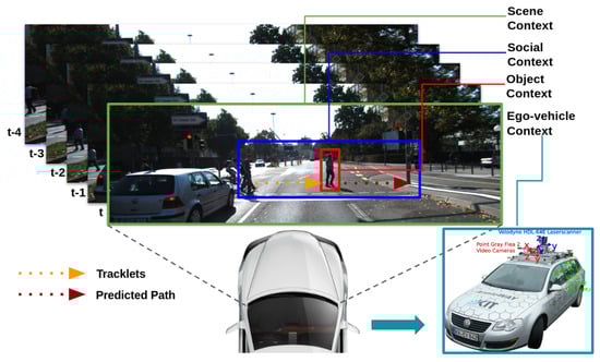
Figure 1.
Contextual information.
For traffic scenes, and specifically from cameras mounted on a moving vehicle, the following features were used: object, ego-vehicle telemetery data, scene, and interaction-aware or social context features (other objects), as visualised in Figure 1. These four types of features were selected since they cover most of the information that can be obtained from the perspective of an ego vehicle.
Object. Besides the position of the object, regions of the objects from the RGB images are used. These cropped images can potentially provide a better understanding of the object, such as the pose or orientation that can be leveraged as additional features.
Ego Vehicle. The following features were selected because they are more related to the movement of the vehicle on the ground. Yaw: heading (rad), VF: forward velocity, VL: leftward velocity, VU: upward velocity, AF: forward acceleration, AL: leftward acceleration, AU: upward acceleration.
Scene. Including information about the scene can potentially help to understand the type of traffic scene where the prediction is happening. In this work, RGB images are used.
Interaction Aware. Taking into account the position of other objects is an important feature for path prediction that is called interaction awareness. In this work, three representations of the position of the objects in a scene are used—a grid map, a polar map, and a local BEV map of objects. The grid and the polar map are implemented as in [13]. A Local Bird’s-Eye View Map represents in pixels the position of the objects in the real world. The map encodes the type of each object in a specific color; red for pedestrian, green for vehicles, and blue for cyclists. Here, we used a scale of 1 px:0.3 m because it helps to better separate objects that are too close to one another. However, the BEV contains all the objects in a scene, but for predicting the path of an object, nearby objects are the most influential. Therefore, a local BEV is extracted from the global BEV, as in Figure 2.
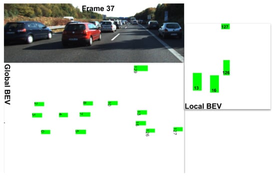
Figure 2.
Local BEV for object ID 126.
3.2. Feature Extraction
Taking into account the related works, three CNN models were created to process each type of image in this work. Figure 3 details the model used to process the object image. The architecture is the same for the other type of images—the only difference is the shape, since the sizes of the other types of images are different. For comparison, based on information in [20]—“The responses from the higher-level layers of CNN (e.g., fc6, fc7 from AlexNet) have been shown to be very effective generic features with state-of-the-art performance on a variety of image datasets” (p. 5)—and for its use in [13], we decided to use AlexNet to compare performance with our proposed CNN models. Figure 4 presents the AlexNet architecture for the object image. The architecture is the same for the other type of images, the difference is the stride in the conv1 and maxPool1 layers which is as follows: the interaction-aware image strides for conv1 and maxPool1 are 4 and 1, respectively. For the scene image, the strides for conv1 and maxPool1 are 3 and 2, respectively.
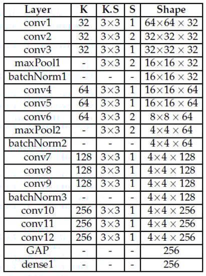
Figure 3.
4block3convGAP.
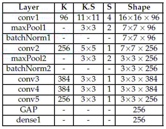
Figure 4.
AlexNet.
3.3. Fusion Strategies
The following three fusion strategies are evaluated: (1) early fusion of raw features (RF), (2) early fusion of latent space (LS) features, (3) middle fusion of latent space (LS) features. The architecture for each type of fusion is presented in the experiments.
3.4. Evaluation Metrics
As in [25,26], the Average Displacement Error (ADE) and Final Displacement Error (FDE) are used:
where are the predicted positions of the tracklet i at time t, are the actual position (ground truth) of the tracklet i at time t, is the last prediction step, and n is the number of tracklets in the testing set. We used the weighted sum of ADE (WSADE) and weighted sum of FDE (WSFDE) as metrics, as shown in (http://apolloscape.auto/trajectory.html (accessed on 10 February 2023)).
3.5. Model Architecture
The focus of this research is to demonstrate the improvement of the path prediction task when using more features, which is why two foundational architectures were used. Each LSTM has 128 units using the default Keras’ configuration. The Adam optimizer was also used with the default values. For regression loss, the Mean Squared Error (MSE) was used. All experiments were run for 1000 epochs, except for those where an initial evaluation of CNN models was performed (300 epochs). The batch size used was 32 due to hardware limitations and because using a small batch size leads to a better trained model. The architecture of the models changes according to the features and are illustrated in their respective sections below:
- Vanilla LSTM:an LSTM using the default Keras’ configuration.
- Encoder–Decoder: the encoder comprises a vanilla LSTM for numerical data and a CNN+LSTM for image data. The decoder is a vanilla LSTM that is fed with the features or concatenation of features from the encoder.
4. Experimental Setup
The dataset used to evaluate the models was KITTI due to its realistic scenes, such as highways, inner cities, vehicles standing/moving, and its different objects. All this information is obtained from cameras mounted on a vehicle, which is the main focus of this research work. There are other datasets, however, that do not provide RGB images of the scenarios and ego vehicle features as KITTI does. KITTI provides information from different type of sensors that can be fused and used together. The size of the dataset is 20,141 samples with a class distribution of cyclists (802), pedestrians (6312) and vehicles (13,027). The evaluation was carried out using three objects—pedestrian, vehicles, and cyclists—for a prediction horizon (P.H.) of ±20 steps. The available dataset is not large and no standard test/train split is available. For this reason, 5-fold cross validation was carried out and the mean results are reported.
4.1. Data Pre-Processing
KITTI provides the data in different files; to use these features together, all the information was synchronized, with the time stamp/ID reference taken as the frame number of each measurement. Each type of data was processed as follows:
- Object: position in metres were extracted. RGB features: patches of the objects were extracted and resized to 64 × 64 pixels.
- Ego vehicle: orientation, velocity in , acceleration in features were extracted from the oxt files which are the dynamics of the ego vehicle.
- Scene: RGB images from the scenes were resized to 124 × 37 pixels.
- Interaction aware: grid and polar map were flattened first to feed an LSTM. The local image BEV map was resized to 40 × 40 pixels.
4.2. Training and Prediction
During training, cross validation with was carried out and for each fold a training and test split was performed with 70% of the data used for training and the rest for testing. Additionally, to feed the model correctly, the following steps were performed:
- Select the features to use: object image, ego-vehicle information, scene image and interaction-aware information can be used.
- Scale data: tracklets were scaled to [0, 1]. Images were divided by 255 before being fed to the CNN models.
- Split data into observed tracklet, , and ground truth tracklet (path to be predicted), . is shaped as [, , ] and as [, ]. is the size of the output of the model. In this case, . Here, represents the steps to predict in the future and is the number of features to predict in each step.
In [2], it was shown that LSTMs can be extended to predict multiple paths by combining them with Mixture Density Models (MDMs) as a final layer. However, in this work, a single path was predicted to better analyse the impact of the contextual features. The model outputs a single array, , per of size . is re-shaped to .
5. Exploration of Multimodal Features
Several combinations of pairs of features were tested; then, those features that led to better performance were selected to create a combination of three features. Due to hardware limitations and the lack of improvement when fusing three type of features, no further combinations were tested.
The results are visualised using a colour scaling in a range of white to red. A white background means that the model achieved the best performance and a red background means that model showed the worst performance. A reddish shade means the model’s performance is between the best and the worst. The second column shows WSADE, followed by the individual ADE for each type of object. The fifth column presents WSFDE, followed by the individual FDE for each type of object.
Experiments and Results
X, Y Features. This experiment consists of feeding an LSTM with raw features versus first encoding the raw features in a latent space with an LSTM (the encoder) and then feeding this into another LSTM (the decoder). The results depicted in Figure 5 demonstrate that encoding the raw features in latent space improves performance over using the raw features to feed the Vanilla LSTM.
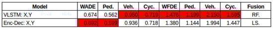
Figure 5.
Raw features vs. latent space features: features.
X, Y, Ego-vehicle Features. Three combinations of ego vehicle information were evaluated—1. [x,y,VF,VL], 2. [x,y,VF,VL,AF,AL] and 3. [x,y, HEADING, VF,VL,AF,AL]. To explore these features further, three fusion strategies were tested. From the results shown in Figure 6, two observations can be drawn: (1) the combination of features: the results indicate that using and VF, VL, AF and AL reduces the error in the prediction. (2) Fusion strategy: in most of the cases, using the middle fusion of features’ latent space improves performance. On the contrary, using the raw features directly to feed the LSTM leads to a greater error.
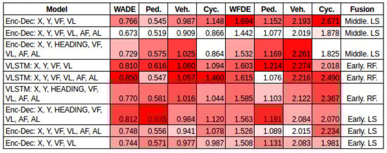
Figure 6.
Early fusion raw features, early fusion latent space, middle fusion latent space: , ego-vehicle features.
The models used to fuse the information in this experiment in three different strategies—early fusion no latent space, early fusion latent space and, middle fusion latent space—are presented in Figure 7, Figure 8, Figure 9, respectively. The figures show the fusion of four features—VF, VL, AF, AL of the ego vehicle—the fusion with the other two combinations—VF, VL and Heading, VF, VL, AF, AL—follow the same architecture.
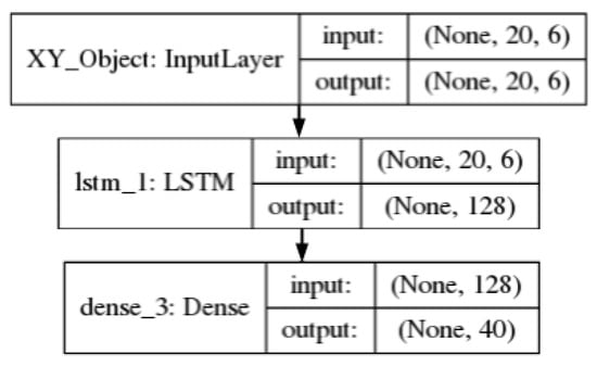
Figure 7.
Early fusion no latent space: and vf, vl, af, al features.
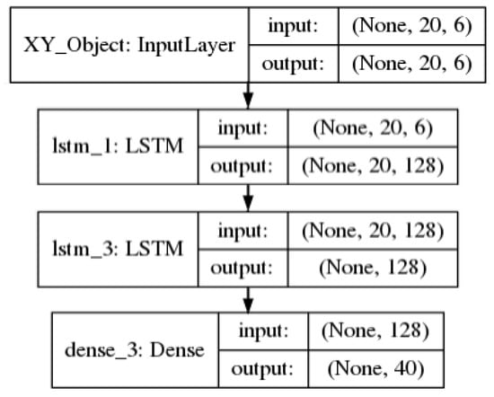
Figure 8.
Early fusion latent space: and vf, vl, af, al features.
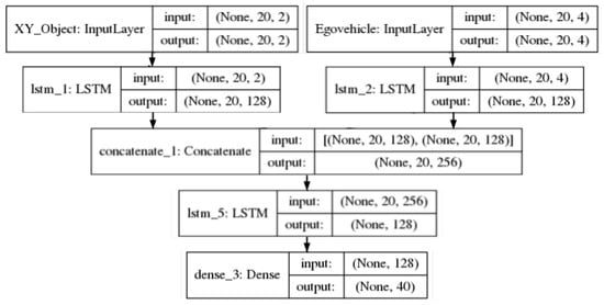
Figure 9.
Middle fusion latent space: and vf, vl, af, al features.
X, Y, Object Image. The initial approach to include deep features was to use the model from SSLSTM [13], where the code (https://github.com/xuehaouwa/SS-LSTM (accessed on 15 February 2023)) is provided. They use AlexNet without the two layers of Conv2D (384), which creates a shallow and narrow CNN model (AlexNet light). The results of this evaluation show no improvement in comparison to the baseline (using only features). The next step was to find out if using a different CNN would improve the performance; therefore, based on the available literature [13,17], we selected two CNNs. (1) 4block3convGAP for object image and (2) AlexNetGAP for object image. Due to the computational requirements, to initially test the performance of the models they were run for 300 epochs, using the k-fold numbers 1, 3 and 5. The results shown in Figure 10 indicate that using the CNN model 4block3convGAP leads to better performance.
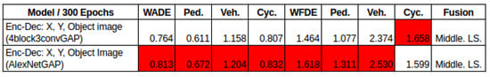
Figure 10.
4block3convGAP vs. AlexNetGAP for object image.
For the second stage of this experiment, the model 4block3convGAP was selected to be run for 1000 epochs and for all the k-folds. The results are shown in Figure 11. It can be observed that the 4block3convGAP CNN significantly improves the performance of the model compared to using the CNN from SSLSTM. Additionally, the 4block3convGAP CNN also improves the performance against the baseline model (using only ). The improvement is mostly seen for FDE, which leads to an error reduction in the prediction of the final position of an object. The improvement reached by using the 4block3convGAP in contrast to the model from SSLSTM provides evidence that refining the CNN model used leads to an improvement in the prediction. The encoder–decoder model used to fuse positional information and the object image is presented in Figure 12.
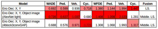
Figure 11.
only vs. AlexNet light vs. 4block3convGAP for object image.
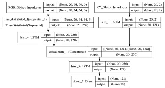
Figure 12.
Fusion model for and object image.
X, Y, Interaction-aware Map. Three types of maps were explored to include other objects’ positional information, a grid map, a polar map, and one local BEV. The results are presented in Figure 13. The following observations can be made: (1) Grid Map vs. Polar Map: using a grid map shows better performance. (2) Fusion strategy: there is a significant error reduction when using middle fusion of features in the latent space. Early fusion, however, leads to a higher error. This is observed for both the grid and polar map.
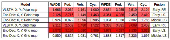
Figure 13.
Early fusion raw features, Early fusion latent space, Middle fusion latent space: , int-aware features.
For the third map BEV, as in X, Y, Object Image, two CNN models were selected—4block3convGAP and AlexNetGAP—for the BEV image. The two CNNs were run for 300 epochs using the k-folds numbers 1, 3 and 5 and the mean are reported in Figure 14. It can be seen that AlexNetGAP is slightly better than 4block3convGAP.
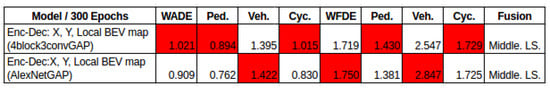
Figure 14.
4block3convGAP vs. AlexNetGAP for interaction-aware local BEV map.
The next step was to train the AlexNetGAP for 1000 epochs on the 5 folds. The results are depicted in Figure 15. It can be observed that using the local BEV with AlexNetGap improves the performance slightly over the use of a grid with middle fusion on latent space. However, the use of local BEV with AlexNetGap does not lead to error reduction over the base line model (using only features). The reason could be because the KITTI dataset does not have many crowded scenes where the objects interact with each other.
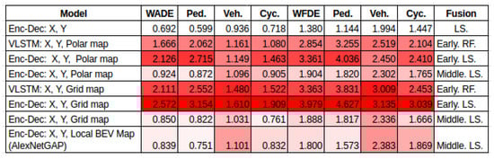
Figure 15.
only vs. polar vs. grid vs. local BEV map.
Three different models were used to fuse positional information and the created handcrafted maps—early fusion with no latent space, early fusion with latent space and middle fusion with latent space. These three models are similar to those used in X, Y, ego-vehicle features (Figure 7, Figure 8, Figure 9, respectively.) The only difference is that in this case the features used are from the created handcrafted maps (grid or polar map). The encoder–decoder model used to fuse positional information and the local BEV map image is similar to the one presented in Figure 12. The only difference is the CNN model, which in this case is used for the interaction-aware image.
X, Y, Scene Image. This experiment combines RGB images of the scenes with the features of the objects. Again, in this set of experiments, we first tested two CNN models (4block3convGAP and AlexNetGAP) for 300 epochs on the k-fold numbers 1, 3 and 5. The mean results are presented in Figure 16. Since AlexNetGAP demonstrated better performance, it was trained for 1000 epochs on the 5 folds. The results are depicted in Figure 17. It can be observed that the use of AlexNetGAP to extract features from scene images leads to a slight error reduction in comparison to the baseline model. The improvement is observed for FDE and mostly for the object cyclist. The encoder–decoder model used to fuse positional information and the scene image is similar to the one presented in Figure 12. The only difference is the CNN model, which in this case is the one used for the scene image.
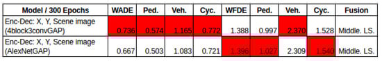
Figure 16.
4block3convGAP vs. AlexNetGAP for scene image.
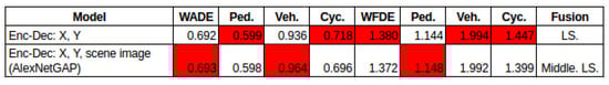
Figure 17.
and scene image: only vs. AlexNetGap for scene image.
Combinations of Features that Lead to a Better Performance. The Figure 18 shows the performance of the baseline model in the first row compared to the two best combinations of features. It can be seen that combining the features with the ego vehicle information (VF, VL, AF, AL) (second row) leads to better performance. The combination of features with the object image also improves the performance against the baseline.
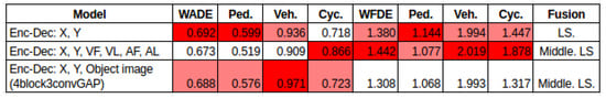
Figure 18.
Combinations of features that lead to a better performance.
X, Y, Object Image, Ego-vehicle Features. Previous experiments shown that ego vehicle information and visual information of the object lead to an error reduction. In this experiment, those two features are combined with the positional information. The results are presented in Figure 19, it can be seen that no improvement was reached when combining these three features. The model architecture is similar to the one shown in Figure 12 but in this case we added another branch of information coming from the ego-vehicle feature, as in Figure 9.
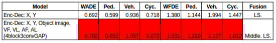
Figure 19.
Combination of three features: , object image, and ego-vehicle.
Ensembles. Three ensembles were built using the models that showed improvement in performance compared to our baseline methodology. Ensemble 1: [Enc-Dec: X, Y], [Enc-Dec: X, Y, VF, VL, AF, AL]. Ensemble 2: [Enc-Dec: X, Y], [Enc-Dec: X, Y, Object image (4block3convGAP)]. Ensemble 3: [Enc-Dec: X, Y], [Enc-Dec: X, Y, VF, VL, AF, AL], [Enc-Dec: X, Y, Object image (4block3convGAP)]. In each ensemble, the output of each model is combined by averaging in the final output layer. The results are presented in Figure 20. The three ensembles achieve better performance than the baseline model (row 1) and the two individual combinations of features (rows 2 and 3).
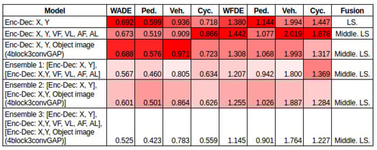
Figure 20.
Results of ensembles.
6. Discussion and Conclusions
The following observations can be noted from exploring multimodal features on the path prediction task:
Best Combination of Features. Combining with the ego-vehicle features leads to a better performance mostly for ADE. The combination of with Object image also improves the performance against the baseline model for both ADE and FDE.
Latent Space Representation and Fusion Strategies. It can be noted that the way in which the features are fused in the model architecture has a significant impact on the prediction. The initial evidence was presented in X, Y features in Figure 5; the results show that representing the features in a latent space improves the performance compared to using the features directly to the LSTM. Then, evidence was presented in X, Y, Ego-vehicle features; the results in Figure 6 indicate that the middle fusion of features represented in latent space had better performance. On the contrary, early fusion led to a higher error. Next, evidence was presented in X, Y, interaction-aware map; the results exhibited in Figure 13 revealed that there is an error reduction when using middle fusion in the latent space. Again, early fusion led to a higher error. Looking at the impact of the fusion strategies, it would be interesting to explore more in this area, since not only are the features important, but the way these features are fused in a model architecture is also of importance.
CNN Models. From the three experiments in which deep features were used, something important to point out is the impact that a CNN model has in the overall path prediction task. When dealing with images, an evaluation of different CNNs is desirable. It would be interesting to evaluate more CNNs and to see if some of them with common characteristics such as the number of CNN layers, filter size, or specific type of layers (GAP, Attention, etc.) can improve the performance.
Ensembles. It is known that ensembles improve the performance of individual classifiers or methods; in this work, there is evidenced in the context of path prediction in traffic scenes. The three ensembles improved the performance of the baseline methodology and the two other best individual models.
Author Contributions
Conceptualization, J.B.F. and S.L.; methodology, J.B.F. and S.L.; data acquisition, J.B.F.; software tools, J.B.F.; validation, J.B.F.; investigation, J.B.F.; writing—original draft preparation, J.B.F.; writing—review and editing, J.B.F., S.L. and N.E.O.; visualization, J.B.F.; supervision, S.L. and N.E.O. All authors have read and agreed to the published version of the manuscript.
Funding
This publication has emanated from research conducted with the financial support of Science Foundation Ireland [12/RC/2289_P2] at Insight the SFI Research Centre for Data Analytics at Dublin City University.
Institutional Review Board Statement
Not applicable.
Informed Consent Statement
Not applicable.
Data Availability Statement
Not applicable.
Acknowledgments
The GPU GeForce GTX 980 used for this research was donated by the NVIDIA Corporation.
Conflicts of Interest
The authors declare no conflict of interest.
References
- Fernandez, J.B.; Little, S.; O’Connor, N.E. A Single-Shot Approach Using an LSTM for Moving Object Path Prediction. In Proceedings of the 2019 Ninth International Conference on Image Processing Theory, Tools and Applications (IPTA), Istanbul, Turkey, 6–9 November 2019; IEEE: Piscataway, NJ, USA, 2019; pp. 1–6. [Google Scholar]
- Fernandez, J.B.; Little, S.; O’connor, N.E. Multiple Path Prediction for Traffic Scenes using LSTMs and Mixture Density Models. In Proceedings of the Proceedings of the 6th International Conference on Vehicle Technology and Intelligent Transport Systems—VEHITS, INSTICC, Prague, Czech Republic, 2–4 May 2020; SciTePress: Setubal, Portugal, 2020; pp. 481–488. [Google Scholar] [CrossRef]
- Jin, X.B.; Su, T.L.; Kong, J.L.; Bai, Y.T.; Miao, B.B.; Dou, C. State-of-the-Art Mobile Intelligence: Enabling Robots to Move Like Humans by Estimating Mobility with Artificial Intelligence. Appl. Sci. 2018, 8, 379. [Google Scholar] [CrossRef]
- Keller, C.G.; Gavrila, D.M. Will the pedestrian cross? A study on pedestrian path prediction. IEEE Trans. Intell. Transp. Syst. 2014, 15, 494–506. [Google Scholar] [CrossRef]
- Bian, J.; Tian, D.; Tang, Y.; Tao, D. A survey on trajectory clustering analysis. arXiv 2018, arXiv:1802.06971. [Google Scholar]
- Zyner, A.; Worrall, S.; Nebot, E. Naturalistic driver intention and path prediction using recurrent neural networks. IEEE Trans. Intell. Transp. Syst. 2019, 21, 1584–1594. [Google Scholar] [CrossRef]
- Altché, F.; de La Fortelle, A. An LSTM network for highway trajectory prediction. In Proceedings of the 2017 IEEE 20th International Conference on Intelligent Transportation Systems (ITSC), Yokohama, Japan, 16–19 October 2017; IEEE: Piscataway, NJ, USA, 2017; pp. 353–359. [Google Scholar]
- Park, S.H.; Kim, B.; Kang, C.M.; Chung, C.C.; Choi, J.W. Sequence-to-sequence prediction of vehicle trajectory via LSTM encoder-decoder architecture. In Proceedings of the 2018 IEEE Intelligent Vehicles Symposium (IV), Suzhou, China, 26–30 June 2018; IEEE: Piscataway, NJ, USA, 2018; pp. 1672–1678. [Google Scholar]
- Bartoli, F.; Lisanti, G.; Ballan, L.; Del Bimbo, A. Context-aware trajectory prediction. In Proceedings of the 2018 24th International Conference on Pattern Recognition (ICPR), Beijing, China, 20–24 August 2018; IEEE: Piscataway, NJ, USA, 2018; pp. 1941–1946. [Google Scholar]
- Kim, B.; Kang, C.M.; Kim, J.; Lee, S.H.; Chung, C.C.; Choi, J.W. Probabilistic vehicle trajectory prediction over occupancy grid map via recurrent neural network. In Proceedings of the 2017 IEEE 20th International Conference on Intelligent Transportation Systems (ITSC), Yokohama, Japan, 16–19 October 2017; IEEE: Piscataway, NJ, USA, 2017; pp. 399–404. [Google Scholar]
- Bhattacharyya, A.; Fritz, M.; Schiele, B. Long-term on-board prediction of pedestrians in traffic scenes. In Proceedings of the 1st Conference on Robot Learning, Mountain View, CA, USA, 13–15 November 2017. [Google Scholar]
- Pool, E.A.; Kooij, J.F.; Gavrila, D.M. Context-based cyclist path prediction using recurrent neural networks. In Proceedings of the 2019 IEEE Intelligent Vehicles Symposium (IV), Paris, France, 9–12 June 2019; IEEE: Piscataway, NJ, USA, 2019; pp. 824–830. [Google Scholar]
- Xue, H.; Huynh, D.Q.; Reynolds, M. SS-LSTM: A hierarchical LSTM model for pedestrian trajectory prediction. In Proceedings of the 2018 IEEE Winter Conference on Applications of Computer Vision (WACV), Lake Tahoe, NV, USA, 12–15 March 2017; IEEE: Piscataway, NJ, USA, 2018; pp. 1186–1194. [Google Scholar]
- Cui, H.; Radosavljevic, V.; Chou, F.C.; Lin, T.H.; Nguyen, T.; Huang, T.K.; Schneider, J.; Djuric, N. Multimodal trajectory predictions for autonomous driving using deep convolutional networks. In Proceedings of the 2019 International Conference on Robotics and Automation (ICRA), Montreal, QC, Canada, 20–24 May 2019; IEEE: Piscataway, NJ, USA, 2019; pp. 2090–2096. [Google Scholar]
- Lee, N.; Choi, W.; Vernaza, P.; Choy, C.B.; Torr, P.H.; Chandraker, M. Desire: Distant future prediction in dynamic scenes with interacting agents. In Proceedings of the IEEE Conference on Computer Vision and Pattern Recognition, Honolulu, HI, USA, 21–26 July 2017; pp. 336–345. [Google Scholar]
- Bighashdel, A.; Dubbelman, G. A survey on path prediction techniques for vulnerable road users: From traditional to deep-learning approaches. In Proceedings of the 2019 IEEE Intelligent Transportation Systems Conference (ITSC), Auckland, New Zealand, 27–30 October 2019; IEEE: Piscataway, NJ, USA, 2019; pp. 1039–1046. [Google Scholar]
- Sharif, M.; Kausar, A.; Park, J.; Shin, D.R. Tiny image classification using Four-Block convolutional neural network. In Proceedings of the 2019 International Conference on Information and Communication Technology Convergence (ICTC), Jeju Island, Republic of Korea, 16–18 October 2019; IEEE: Piscataway, NJ, USA, 2019; pp. 1–6. [Google Scholar]
- Yao, L.; Miller, J. Tiny imagenet classification with convolutional neural networks. CS 231N 2015, 2, 8. [Google Scholar]
- Abai, Z.; Rajmalwar, N. DenseNet Models for Tiny ImageNet Classification. arXiv 2019, arXiv:1904.10429. [Google Scholar]
- Zhou, B.; Khosla, A.; Lapedriza, A.; Oliva, A.; Torralba, A. Learning deep features for discriminative localization. In Proceedings of the IEEE Conference on Computer Vision and Pattern Recognition, Las Vegas, NV, USA, 27–30 June 2016; pp. 2921–2929. [Google Scholar]
- Ioffe, S.; Szegedy, C. Batch normalization: Accelerating deep network training by reducing internal covariate shift. In Proceedings of the International Conference on Machine Learning, Lille, France, 6–11 July 2015; PMLR: Cambridge, MA, USA, 2015; pp. 448–456. [Google Scholar]
- Garbin, C.; Zhu, X.; Marques, O. Dropout vs. batch normalization: An empirical study of their impact to deep learning. Multimed. Tools Appl. 2020, 79, 12777–12815. [Google Scholar] [CrossRef]
- Hu, Y.; Lu, M.; Lu, X. Spatial-Temporal Fusion Convolutional Neural Network for Simulated Driving Behavior Recognition. In Proceedings of the 2018 15th International Conference on Control, Automation, Robotics and Vision (ICARCV), Singapore, 18–21 November 2018; IEEE: Piscataway, NJ, USA, 2018; pp. 1271–1277. [Google Scholar]
- Roitberg, A.; Pollert, T.; Haurilet, M.; Martin, M.; Stiefelhagen, R. Analysis of deep fusion strategies for multi-modal gesture recognition. In Proceedings of the Proceedings of the IEEE/CVF Conference on Computer Vision and Pattern Recognition Workshops, Long Beach, CA, USA, 15–20 June 2019. [Google Scholar]
- Hou, L.; Xin, L.; Li, S.E.; Cheng, B.; Wang, W. Interactive trajectory prediction of surrounding road users for autonomous driving using structural-LSTM network. IEEE Trans. Intell. Transp. Syst. 2019, 21, 4615–4625. [Google Scholar] [CrossRef]
- Ma, Y.; Zhu, X.; Zhang, S.; Yang, R.; Wang, W.; Manocha, D. Trafficpredict: Trajectory prediction for heterogeneous traffic-agents. In Proceedings of the Proceedings of the AAAI Conference on Artificial Intelligence, Honolulu, HI, USA, 27 January–1 February 2019; Volume 33, pp. 6120–6127.


Disclaimer/Publisher’s Note: The statements, opinions and data contained in all publications are solely those of the individual author(s) and contributor(s) and not of MDPI and/or the editor(s). MDPI and/or the editor(s) disclaim responsibility for any injury to people or property resulting from any ideas, methods, instructions or products referred to in the content. |
© 2023 by the authors. Licensee MDPI, Basel, Switzerland. This article is an open access article distributed under the terms and conditions of the Creative Commons Attribution (CC BY) license (https://creativecommons.org/licenses/by/4.0/).