Abstract
During the first year of the COVID-19 pandemic, governments only had access to non-pharmaceutical interventions (NPIs) to mitigate the spread of the disease. Various methods have been discussed in the literature for calculating the effectiveness of NPIs. Among these methods, the interrupted time series analysis method is the area of our interest. To study the second wave, we clustered countries based on levels of implemented NPIs, except for the target NPI (X) whose effectiveness wanted to be evaluated. To do so, the COVID-19 Policy Response Tracker data-set gathered by the “Our World in Data” team of Oxford University, and COVID-19 statistical data gathered by the John Hopkins Hospital were used. After clustering, we selected a counterfactual country from the countries that were in the same cluster as the target country, and implemented NPI (X) at its lowest level. Thus, the target country and the counterfactual country were similar in implementation level of other NPIs and only differed in the implementation level of the target NPI (X). Therefore, we can calculate the effectiveness of NPI (X) without being concerned about the impurity of the effectiveness values that might be caused by other NPIs. This allowed us to calculate the effectiveness of NPI (X) using the interrupted time series analysis with the control group. Interrupted time series analysis assesses the effect of different policy-implementation levels by evaluating interruptions caused by policies in trend and level after the policy-implementation date. Before the NPI-implementation date, the implementation levels of NPIs were similar in both selected countries. After this date, the counterfactual country could be treated as a baseline for calculating changes in the trends and levels of COVID-19 cases in the target country. To demonstrate this approach, we used the generalized least square (GLS) method to estimate interrupted time series parameters related to the effectiveness of school closure (the target NPI) in Spain (the target country). The results show that increasing the implementation level of school closure caused a 34% decrease in COVID-19 prevalence in Spain after only 10 days compared to the counterfactual country.
1. Introduction
The highly transmissible COVID-19 virus was announced as a variant of concern (VoC) by the World Health Organization (WHO) on the 11 March 2020 [1]. During the first year of the COVID-19 pandemic, governments used non-pharmaceutical interventions (NPIs) to control the spread of COVID-19, in the absence of medications and vaccines.
Restrictive NPIs can be categorized at the individual level, such as face covering mandates, and the social level, i.e., public transport restrictions, school closure, workplace closure, public event cancelations, restrictions on gatherings, stay-at-home orders, and international travel bans. Researchers have applied various methodologies to assess the effectiveness of these NPIs. Previous research has shown that even after developing and administering the COVID-19 vaccine and before achieving herd immunity, the NPIs remained effective [1].
Navazi et al. [1] analyzed the effects of lockdown on the third wave of COVID-19 in the province of Ontario, Canada, using the interrupted time series analysis (ITSA) method considering vaccination percentage; however, they did not have a counterfactual baseline to calculate lockdown effectiveness and only relied on predicting what would happen in the future, based on pre-intervention trends. Conversely, having a counterfactual country is more realistic. Saki et al. [2] found ITSA to be effective in estimating the effectiveness of social distancing in Iran. However, a limitation of their work was that they assumed the relationship between NPI implementation and COVID-19 confirmed cases to be linear, while it is known that epidemics follow a non-linear trend. This led us to add some non-linear terms to our model.
Auger et al. [3] also used ITSA to estimate the effectiveness of school closure. Although they added some of the other NPIs as covariates to their model, the effectiveness of school closure was not calculated independently and might depend on other NPI implementation levels. Therefore, in this study, we used ITSA with a control group to isolate the effectiveness of the NPI. Thayer et al. [4] used ITSA to investigate the effectiveness of lockdown in India. They considered lockdown implementation levels and estimated the effectiveness of different levels of lockdown. However, their research was limited to a single country, whereas when several countries with similar NPI-implementation levels exist, they can be used for ITSA with a control group. Emeto et al. [5] used ITSA with a matched-control country to study the effectiveness of border closure in Africa. However, the multi-country study by Ballard et al. [6] only considered the region as the ITSA model’s input variable, not as a control group. Shah et al. [7] applied ITSA individually to three regions and compared the impact of the first lockdown on non-COVID-19 patient hospital admission in these three regions. In this case, they implemented single-group ITSA three times without an accompanying counterfactual analysis.
There are some challenges in single-group interrupted time series analysis, such as being unable to control for other competing factors [8], poor internal validity [8], or using treatment group pre-intervention trends as counterfactuals [5]. To solve these issues, we will use other ITSA designs, such as using a control group, to obtain valid and causal results.
We developed a clustering-based counterfactual selection integrated with an interrupted time series analysis with a control group to address the research gap. For example, if we consider eight main restrictive NPIs to study, we will cluster countries based on seven NPIs. The remaining NPI (X) is the one whose effectiveness we are interested in studying. The selection mechanism of the control country was based on two criteria: (1) being in the same cluster as the target country and (2) having the greatest difference with the target country in implementing NPI (X) and implementing NPI (X) at a zero or lower level. Having a comparable control group helps to implement a robust approach that considers treatment effects [8]. This way, the change in COVID-19 prevalence resulting from the pattern of a COVID-19 wave, rather than the intervention, is considered, and will not lead to an underestimation or overestimation of the number of COVID-19 cases [8].
Regarding wave selection, if we are interested in studying the effectiveness of both non-pharmaceutical interventions and pharmaceutical interventions such as vaccines, then a wave during 2021 should be selected, whereas if we want to only study the effectiveness of NPIs, we should select the first or second wave of COVID-19 during 2020. As the first COVID-19 wave’s statistics have many uncertainties resulting from the shortage of test kits and non-standard COVID-19 diagnosis methods [1], we will focus on a study of the second wave of COVID-19.
2. Materials
This study used time series data from 8 NPIs in the COVID-19 Policy Response Tracker of Oxford University [9]. Effectiveness of the NPI that we are interested in studying is school closure, which means students and teachers are not required to go to school for in-person activities, and educational activities are provided online (except for some lab research) [3]. The 8 NPI implementation levels are as follows:
- Public event cancelation implemented at 3 levels: no measure (0), recommended cancelation (1), and required cancelation (2).
- Restrictions on gatherings, which limits the number of people in gatherings to less than 10 (4), 10 to 100 (3), 100 to 1000 (2), limiting only very large gatherings (>1000 people) (1), no limit (0) (five levels).
- Workplace closure implemented at four levels: no closure (0), recommended closure (1), required closure for some (2), and required closure for all (3).
- School closure implemented at four levels: no closure (0), recommended closure (1), required closure for some (2), and required closure for all (3).
- Restriction on internal movement is implemented at three levels: no measure (0), recommend movement restriction (1), and required movement restriction (2).
- International travel ban implemented at five levels: no measures (0), screening (1), quarantining of arrivals from high-risk regions (2), banning high-risk regions (3), and total border closure (4).
- Public transport closure implemented at three levels: no measures (0), recommend closing (or significantly reduced volume/route/means of available transport) (1), required closure (or prohibiting most people from using it) (2).
- Stay-at-home requirements implemented at four levels, including no measure (0), recommending not leaving the house (1); requiring not leaving the house, with exceptions for grocery shopping, essential trips, etc. (2); requiring not leaving the house with minimal exceptions like once every few days, etc. (3).
The COVID-19 statistical data, including COVID-19 prevalence provided by John Hopkins Hospital [10], was also used. Additionally, we calculated a date column showing how many days had passed since the start of the second wave.
3. Methods
Interrupted time series analysis is a statistical methodology used to study intervention effects that can cause both level and trend changes [1]. When only one group is exposed to the policy, researchers use a “pre-post” observational study design. However, if we have two groups and only one is exposed to the policy, we can use a “pre-post with control” observational study design. One group without exposure to the policy works as a control group for the other. This method is also called a difference in differences study. Having a control country helps to capture the change in trend caused by policy instead of the nonlinearity (curvilinear) of the outcome wave. Since adding a control group solidifies the study, we will use this research design.
In order to determine what would have happened if there had been no NPI X (target NPI to study its effectiveness), we needed a counterfactual country that did not implement NPI X but implemented the rest of the NPIs at a similar level with the target country. This method is called counterfactual analysis. Therefore, we developed a hybrid methodology with clustering-based counterfactual selection to find a suitable control group for interrupted time series analysis with control, as hybrid methodologies are well known for covering the shortcomings of a methodology with a second method [11].
First, we clustered all countries with their data based on all studied NPIs except for NPI X. The K-Means clustering algorithm [12] was used for this purpose. This identifies which countries are in the same cluster as the target country. Among these countries, we determined pairs of countries that implemented NPI X at different levels. We then looked at the countries paired with the target country and selected the country which could work as a control group. A control country must have implemented NPI X at zero or lower levels for a period before and after NPI X implementation level changes in the target country. After selecting the control country estimate, we could use interrupted time series with counterfactual analysis for the control group to determine the effectiveness of NPI X. The methodology’s steps are illustrated in Figure 1.
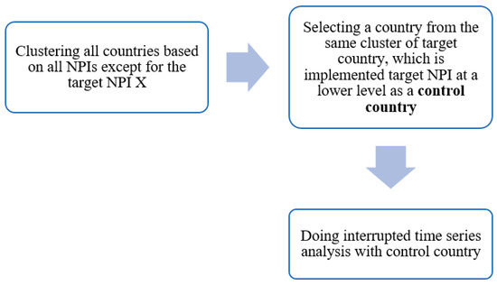
Figure 1.
Developed hybrid methodology.
We have data from several populous European countries, including Austria, Belgium, Czechia, Denmark, Finland, France, Germany, Italy, Netherlands, Norway, Poland, Portugal, Romania, Russia, Spain, Switzerland, United Kingdom, available to select the target and control countries.
In this study, the second wave of COVID-19, which occurred at the end of 2020 and the beginning of 2021 in most countries, was studied. This is because COVID-19 vaccines, developed at the beginning of 2021, affected immunization, while we want to study NPIs, not pharmaceutical interventions. Moreover, clustering by considering vaccine administration percentage is difficult given vaccine shortages at the beginning of 2021, countries varied in vaccine administration percentage, and it is hard to cluster countries based on pharmaceutical interventions and NPIs at the same time.
The target country of this study is Spain, and the target NPI whose effectiveness is investigated is school closure. We focused on finding a control country that implemented school closure at a lower level by clustering countries based on other NPIs.
We clustered countries based on NPIs mentioned in the Materials section, except for school closure. Since the data related to each NPI are time series data during the second wave of COVID-19, the problem was clustering time series data. One of the methods for clustering time series data is considering each time point as a data column (feature) for clustering. Figure 2 illustrates how the data frame was transformed for time series clustering purposes. We considered just the first 60 days of the second wave because the performance of K-Means depends on the number of features, and it cannot perform well when the number of features is increased [13]. Moreover, the minimum duration for the second COVID-19 wave was 65 days in Poland.
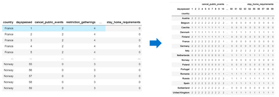
Figure 2.
Data frame transformation for time series clustering.
The time series clustering was coded in Python 3.8, and the K-Means algorithm from Python’s Scikit-learn library was used. Since we wanted to cluster time series data, dynamic time wrapping (DTW) distance [13] was used for calculating the distance among points and cluster centroids instead of simple Euclidean distance in the body of the K-Means algorithm. Euclidean distance ignores the time dimension of data and cannot take into account time shifts, whereas dynamic time wrapping can handle these features [13].
One of the limitations of K-Means clustering is that the number of clusters (K) is not determined. Several ways exist to determine the number of clusters, like elbow law or Silhouette score. Here, we used Silhouette score, which measures how well the items (countries) in one cluster are separated from items (countries) in another cluster. The maximum Silhouette score is one, and it assigns higher values to better clustering results [13]. Figure 3 illustrates the Silhouette metrics for different numbers of clusters. Since we had 17 countries to cluster, the maximum number of clusters was set to 9 because we needed at least one pair of countries in each cluster in order to select the control country. Since K = 2 has the highest Silhouette score, we set the number of clusters at 2.
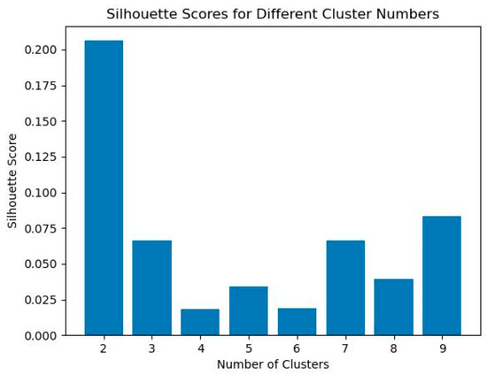
Figure 3.
Determining the number of clusters by Silhouette score.
The K-Means algorithm clustered the given countries in 2 clusters, as illustrated in Figure 4.
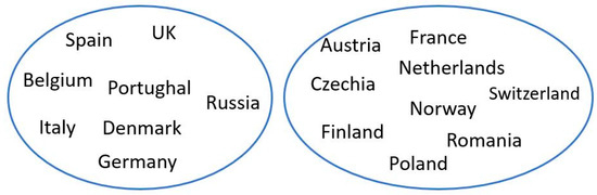
Figure 4.
Clustering (K = 2) results for the second wave of COVID-19.
In order to select the counterfactual country from the cluster that Spain is in, a loop was coded in Python that paired all countries in the cluster with Spain. Then, this loop checked for a significant difference between the mean [14] of NPI X implementation levels in each pair. Statistical paired t-test was used to check the mean difference [11]. This helped to select the counterfactual country. Table 1 shows all countries paired with Spain, the mean difference in school closure implementation level, and the p-value of the t-test.

Table 1.
t-test results for the mean difference of NPI (X).
Belgium and Denmark had the highest difference in implementing school closure. Between these two countries, we found Belgium to be the more suitable country as a control group. While Spain changed the school closure implementation level from 2 to 3 on day 101 of the second wave, Belgium changed its level from 1 to 2 on day 109 of the second wave. However, in Denmark, the school closure implementation level changed from 2 to 1 on day 24 of the second wave, again from 1 to 0 on day 105 of the second wave, and from 0 to 2 on day 124 of the second wave. As there was more fluctuation in school closure implementation levels in Denmark, Belgium seemed a better option for counterfactual analysis. Moreover, at least one level difference exists between school closure implementations in Spain and Belgium. This allowed us to investigate the effectiveness of higher-level school closure implementations using interrupted time series analysis with Belgium as a control country.
Interrupted time series analysis was implemented using NLME [15] and CAR [16] libraries of the RStudio software version 1.4.1106. The interrupted time series model that we wanted to analyze is as follows:
TC is the Target Country, a binary variable showing whether it is an intervention country (1) or a control country (0). By integrating clustering-based counterfactual analysis with interrupted time series analysis, we could overcome some of the drawbacks of interrupted time series stated in [17], such as the difficulty of isolating one policy’s effect. So, it is effective to have a control group.
We found the periods of the autoregressive residual and moving average by doing a preliminary interrupted time series analysis. The ordinary least squares (OLS) method was used for preliminary interrupted time series analysis. R squared of the GLS model was 72%, which meant that 72% of COVID-19 prevalence could be explained by the input variables, including days passed since the beginning of the second COVID-19 wave and the NPI implementation levels. Since OLS assumes the error terms are independent, we found suitable periods for autoregression or moving averages by checking for autocorrelation.
To check for autocorrelation, the auto correlation function (ACF) plot and partial ACF (PACF) plot of the OLS model residuals are illustrated in Figure 5. We considered the maximum 23-day possible lag. Since ACF shows exponential decay, we utilized autoregression (AR). AR means that the error term is related to the error term in previous periods. Since PACF does not show an exponential decay, considering the moving average was not necessary. We examined the PACF plot to determine the AR order and pick the highest violation from the 95% two-way confidence interval (dashed lines). As the PACF for number 7 was larger, AR = 7 was considered for the model.
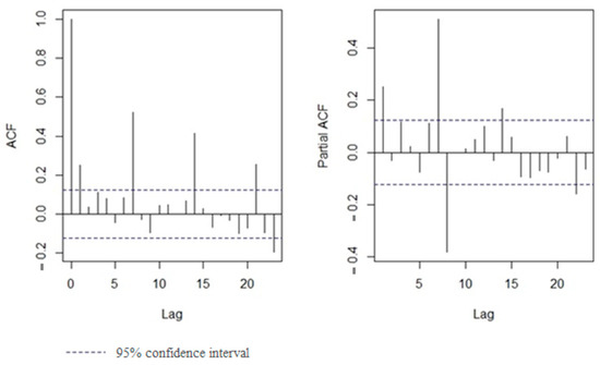
Figure 5.
ACF and PACF plot of OLS model residuals.
The second method for checking autocorrelation was the Durbin–Watson test. The Durbin–Watson test which used to check autoregressive residuals confirmed AR (7). The ideal value for the statistical Durbin–Watson test is 2. If the statistics are above 2, it shows a positive correlation; if they are below 2, it shows a negative correlation [16]. Results of the Durbin–Watson test reported in Table 2 confirms 7 days of lag for autoregression with the lowest absolute statistics (0.9090) and zero p-value (p-value < 0.01).
Table 2.
Durbin–Watson test results.
4. Results and Discussion
After preliminary analysis, we used the generalized least square (GLS) method, which, is an extension of the OLS model that considers both moving average and autoregressive errors [16]. The GLS model’s coefficients and their p-values are reported in Table 3. The residual standard error for this model is 217.9.
Table 3.
GLS results with AR = 7.
In the following, we provide the interpretation of the significant coefficients with a p-value less than 0.05. The COVID-19 prevalence in the control group increased (8.4 units per time period). However, in the target group, it was 6.1 units less, which means 2.3 (8.4–6.1) units per time period. In other words, Spain had a −6 cases per million decrease per time period compared to Belgium.
Moreover, the level coefficient shows a significant and positive level change in the control group (434). However, the level change coefficient caused by intervention in the target country was −511. Since it is a differential level change, it means that intervention caused an approximately −77 (−511 + 434) decrease in the level of COVID-19 prevalence in the intervention country.
As COVID-19 prevalence follows an exponential pattern in each wave, the trend2 term was added to the model, and its coefficients were significant. This means that the COVID-19 prevalence pattern followed an exponential trend. For the control country, this coefficient was −2.6, and for the target country, it was −0.7 (−2.6 + 1.9); although it was less, it was still negative.
Overall, the school closure intervention led to a reduction in the time coefficient, a negative trend2 coefficient, and a decrease in the level of COVID-19 prevalence; therefore, it was effective. On the other hand, the trend change coefficients in both target and control countries were insignificant.
In Figure 6, the blue line is the Spain data, and the red line is the Belgium data (control group). The dashed blue line shows the counterfactual for Spain based on the control group data (without the time-squared term). The blue line after the vertical black dashed line shows the COVID-19 prevalence after stricter intervention implementation in the target country. As shown in Figure 6, one level stricter school closure decreased the COVID-19 prevalence level and caused a negative trend2.
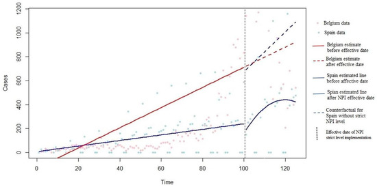
Figure 6.
COVID-19 prevalence in target and control countries with and without school closure level increase.
In order to approximate the effectiveness of one level increase in school closure implementation, we predicted the COVID-19 prevalence 10 days after the school closer level increase, considering intervention (using the main model) and without considering intervention (using the counterfactual model). Ten days were selected, as it takes at least five days (COVID-19 incubation period [18]) to observe the NPI effect on COVID-19 prevalence. The predicted COVID-19 prevalence was 385.5, while its counterfactual equivalent, considering the trend2 coefficient, was 587. This means that one level of school closure increase caused an approximately 34% decrease in COVID-19 prevalence after 10 days, which is significant. Therefore, school closure was an effective NPI.
5. Conclusions
Interrupted time series analysis has been used in the COVID-19 literature to investigate the effectiveness of NPIs. However, the single-group interrupted time series analysis has poor internal validity as well as other shortcomings. In this study, a new statistical methodology was developed and shown to be able to handle these shortcomings. By combining a clustering algorithm with conventional single-group interrupted time series analysis, we found an appropriate control country for our target country and changed the research design to ITSA with a control group. This counterfactual country acted as a baseline for the post-intervention period. Here, a K-Means algorithm was used to cluster countries based on all NPIs except the target NPI with two clusters (K = 2), which had the highest Silhouette score. In our case, Belgium was selected as a control group for Spain, to assess the effectiveness of school closure during the second wave of COVID-19, because it was in the same cluster as Spain and had one of the highest differences in implementing school closure compared with Spain. The interrupted time series with control group results showed that increasing one level of the “School closure” NPI effectively reduced the level and time coefficient of COVID-19 prevalence and maintained the negative trend2 coefficient.
In addition, the ITSA with counterfactual analysis showed that school closure caused a 34% reduction in COVID-19 prevalence 10 days after increasing the level of school closure in Spain. This means that school closure was an effective policy, and adherence to it was important in mitigating the spread of COVID-19. Extending the interrupted time series model to consider adherence to an implemented NPI is an opportunity for future research. Furthermore, improving the performance of the clustering aspect using complex time series clustering methodologies is another future research opportunity. All in all, depending on how many samples are available for clustering, the methodology we developed can also be applied to assessing other public health policies.
Author Contributions
Conceptualization, F.N., Y.Y. and N.A.; methodology, F.N. and N.A.; software, F.N.; validation, F.N.; formal analysis, F.N.; investigation, Y.Y. and N.A.; resources, F.N.; data curation, F.N.; writing—original draft preparation, F.N.; writing—review and editing, N.A. and Y.Y.; visualization, F.N.; supervision, Y.Y. and N.A.; project administration, Y.Y.; funding acquisition, Y.Y. All authors have read and agreed to the published version of the manuscript.
Funding
This research received no external funding.
Institutional Review Board Statement
Not applicable.
Informed Consent Statement
Not applicable.
Data Availability Statement
Data are available at https://ourworldindata.org/policy-responses-COVID.
Conflicts of Interest
The authors declare no conflict of interest.
References
- Navazi, F.; Yuan, Y.; Archer, N. The effect of the Ontario stay-at-home order on COVID-19 third wave infections including vaccination considerations: An interrupted time series analysis. PLoS ONE 2022, 17, e0265549. [Google Scholar] [CrossRef] [PubMed]
- Saki, M.; Ghanbari, M.K.; Behzadifar, M.; Imani-Nasab, M.H.; Behzadifar, M.; Azari, S.; Bakhtiari, A.; Wu, J.; Bragazzi, N.L. The impact of the social distancing policy on COVID-19 incidence cases and deaths in Iran from february 2020 to january 2021: Insights from an interrupted time series analysis. Yale J. Biol. Med. 2021, 94, 13–21. [Google Scholar] [PubMed]
- Auger, K.A.; Shah, S.S.; Richardson, T.; Hartley, D.; Hall, M.; Warniment, A.; Timmons, K.; Bosse, D.; Ferris, S.A.; Brady, P.W.; et al. Association between Statewide School Closure and COVID-19 Incidence and Mortality in the US. JAMA-J. Am. Med. Assoc. 2020, 324, 859–870. [Google Scholar] [CrossRef] [PubMed]
- Thayer, W.M.; Hasan, M.Z.; Sankhla, P.; Gupta, S. An interrupted time series analysis of the lockdown policies in India: A national-level analysis of COVID-19 incidence. Health Policy Plan. 2021, 36, 620–629. [Google Scholar] [CrossRef] [PubMed]
- Emeto, T.I.; Alele, F.O.; Ilesanmi, O.S. Evaluation of the effect of border closure on COVID-19 incidence rates across nine African countries: An interrupted time series study. Trans. R. Soc. Trop. Med. Hyg. 2021, 115, 1174–1183. [Google Scholar] [CrossRef] [PubMed]
- Ballard, M.; Olsen, H.E.; Millear, A.; Yang, J.; Whidden, C.; Yembrick, A.; Thakura, D.; Nuwasiima, A.; Christiansen, M.; Ressler, D.J.; et al. Continuity of community-based healthcare provision during COVID-19: A multicountry interrupted time series analysis. BMJ Open 2022, 12, e052407. [Google Scholar] [CrossRef] [PubMed]
- Shah, S.A.; Brophy, S.; Kennedy, J.; Fisher, L.; Walker, A.; Mackenna, B.; Curtis, H.; Inglesby, P.; Davy, S.; Bacon, S.; et al. Articles Impact of fi rst UK COVID-19 lockdown on hospital admissions: Interrupted time series study of 32 million people. eClinicalMedicine 2022, 49, 101462. [Google Scholar] [CrossRef] [PubMed]
- Linden, A. Challenges to validity in single-group interrupted time series analysis. J. Eval. Clin. Pract. 2017, 23, 413–418. [Google Scholar] [CrossRef] [PubMed]
- Hale, T.; Angrist, N.; Goldszmidt, R.; Kira, B.; Petherick, A.; Phillips, T.; Webster, S.; Cameron-Blake, E.; Hallas, L.; Majumdar, S.; et al. A global panel database of pandemic policies (Oxford COVID-19 Government Response Tracker). Nat. Hum. Behav. 2021, 5, 529–538. [Google Scholar] [CrossRef] [PubMed]
- Johns Hopkins University. Johns Hopkins Coronavirus Resource Center. 2021. Available online: https://coronavirus.jhu.edu/ (accessed on 26 October 2021).
- Navazi, F.; Sazvar, Z.; Tavakkoli-Moghaddam, R. A sustainable closed-loop location-routing-inventory problem for perishable products. Sci. Iran. 2023, 30, 757–783. [Google Scholar] [CrossRef]
- Hartigan, J.A.; Wong, M.A. Algorithm AS 136: A K-Means Clustering Algorithm. J. R. Stat. Soc. Ser. C Appl. Stat. 1979, 28, 100–108. [Google Scholar] [CrossRef]
- Verleysen, M.; François, D. The curse of dimensionality in data mining and time series prediction. In Computational Intelligence and Bioinspired Systems, Proceedings of the 8th International Work-Conference on Artificial Neural Networks, IWANN 2005, Vilanova i la Geltrú, Spain, 8–10 June 2005; Springer: Berlin/Heidelberg, Germany, 2005; pp. 758–770. [Google Scholar]
- Memari, P.; Navazi, F.; Jolai, F. Hybrid wind-municipal solid waste biomass power plant location selection considering waste collection problem: A case study. Energy Sources Part B Econ. Plan. Policy 2021, 16, 719–739. [Google Scholar] [CrossRef]
- Pinheiro, J.; Bates, D.; DebRoy, S.; Sarkar, D.; R Core Team. nlme: Linear and Nonlinear Mixed Effects Models, R Package version 3; R Core Team: Vienna, Austria, 2021; pp. 1–153. Available online: https://cran.r-project.org/package=nlme (accessed on 30 May 2023).
- Fox, J.; Weisberg, S. Time-series regression and generalized least squares: An appendix. In An R Companion to Applied Regression; SAGE: Thousand Oaks, CA, USA, 2018; pp. 1–10. Available online: http://tinyurl.com/carbook (accessed on 28 June 2021).
- Navazi, F.; Yuan, Y.; Archer, N. A review of big data analytics models for assessing nonpharmaceutical interventions for COVID-19 pandemic management. in press.
- Li, Q.; Guan, X.; Wu, P.; Wang, X.; Zhou, L.; Tong, Y.; Ren, R.; Leung, K.S.M.; Lau, E.H.Y.; Wong, J.Y.; et al. Early Transmission Dynamics in Wuhan, China, of Novel Coronavirus–Infected Pneumonia. N. Engl. J. Med. 2020, 382, 1199–1207. [Google Scholar] [CrossRef] [PubMed]


Disclaimer/Publisher’s Note: The statements, opinions and data contained in all publications are solely those of the individual author(s) and contributor(s) and not of MDPI and/or the editor(s). MDPI and/or the editor(s) disclaim responsibility for any injury to people or property resulting from any ideas, methods, instructions or products referred to in the content. |
© 2023 by the authors. Licensee MDPI, Basel, Switzerland. This article is an open access article distributed under the terms and conditions of the Creative Commons Attribution (CC BY) license (https://creativecommons.org/licenses/by/4.0/).