Abstract
The modeling of hydrogeological processes often involves a quantitative description of complex systems in which a limited dataset is available, bringing about the formulation of conceptual models able to describe them in a simplified framework. In order to evaluate the reliability of these conceptual models, a statistical description of the elements composing the system can be useful, especially with reference to their mutual interactions. This study shows, through some applicative examples in the hydrogeological field, that the statistical analysis of characterizing the parameters and cause–effect relations arising from time series monitoring data can give useful information about the system dynamic, thus contributing to updating the conceptual model and therefore improving the results of following numerical modeling. Indeed, this dynamic description of the system, with the introduction of the verification and validation processes of the conceptual model, allows the correction of possible errors due to a lack of data or the phenomenon’s complexity. This leads to many hydrogeological issues, such as the identification of the most productive aquifer or the one that has the highest vulnerability to pollution, as well as zones of interest in groundwater flow that can trigger slope instability.
1. Introduction
Numerical modeling is often used for describing and forecasting the behavior of complex hydrogeological systems, and has several purposes, from water resources management [1], to pollution analysis and related remediation design [2], as well as in slope stability problems [3].
Nevertheless, in mathematical modeling, not all geological and hydrogeological issues can be fully investigated. In fact, most geological phenomena cannot be described by simple predictable quantities (due to cause–effect relationships) on the basis of boundary conditions or as a function of the values obtained from other variables. On the contrary, many typical hydrogeological parameters can be considered as random variables due to:
- the intrinsic variability of natural processes;
- an inability to understand the physical system in its complexity;
- a lack of sufficient data, both in terms of quality and/or quantity [4].
In the applicative field, the hydrogeological complexity of both the system and the processes, and their limited knowledge, can involve unexpected risk, bringing about the need for a different approach in the system characterization [5].
Consequently, when dealing with hydrogeological risk assessment, a statistics-based conceptual model should be considered in order to take into account the different risk scenarios, and therefore to identify the proper mitigation measures.
Conceptual models are simplified descriptions of complex natural-anthropic systems, involving the identification of geomaterials, the reconstruction of their distribution in space, as well as their physical and technical characterization; this characterization is aimed at forecasting the system behavior, by taking into account the main processes which rule it. In fact, based on the conceptual model, the numerical or analytical model can be implemented and afterwards validated; the validation process often involves an improvement in the conceptual model, by means of a refinement in available data or an increasing complexity in the processes description. Regardless, the need for such an improvement must be quantitatively assessed, and this assessment can be efficiently based on time series analysis (i.e., by comparing time series of different parameters, or time series of simulated vs. observed parameters).
This paper proposes some typical hydrogeological situations in which a statistical approach to the conceptual model definition was essential for the reliability of the results of subsequent numerical modeling. With this aim, the hydrogeological system is represented through quantitative conceptual models, in which some elements, and their mutual interactions, are analyzed from a statistical point of view, endeavoring to reproduce the system evolution in a dynamic framework and involving back-analysis upgrading.
2. Conceptual Model Update: From Monitoring Data to Error Detection
In order to implement a statistical framework in which the conceptual model can be dynamically improved, it is necessary to quantify the effect of the modeling error on the forecasting and, therefore, proceed with checks and updates of the model itself, based on monitoring data [6]; the goal is to establish if, and to what extent, the model can explain and predict the observed phenomena, and detect any inconsistencies that require model refinement [7]. Indeed, the mismatch in between the time series of observed values compared to modeling results (values obtained by simulating the system behavior based on the defined conceptual model) should be minimized [8], by taking into account the fact that possible errors can arise from:
- modeling errors—because of incorrect hypotheses in the conceptual model, the model fails in reproducing some processes or some cause–effect relationships;
- parametric errors—due to an insufficient knowledge of the parameters describing the system behavior (i.e., connected to measurement errors, system heterogeneity or incorrect working scale).
The simplest method in order to detect conceptual model errors consists of a graphical comparison between the calculated and observed data [9]; for quantifying the capability of the model to fit the observed data, a goodness-of-fit test can be carried out. More specifically, an analysis of the deviations (i.e., the differences between the observed and simulated data) makes it possible to identify errors together with their typology. In fact, conceptual model errors are systematic and their effects on the modeling results depends on the spatial and temporal scale of the simulation. Consequently, a correlation between residuals over time or space means that a trend exists and, therefore, the model is affected by errors [10]. In more detail, if the residual deviation is constant but not null, the parameters have not been properly calibrated whereas, if it shows a trend, the model setting should be improved; only when it is null can the model be considered acceptable.
This approach has been implemented in a dynamic framework for hydrogeological risk assessment, which accounts for a conceptual model to be updated based on the time series analysis of the residuals (Figure 1). A similar approach had already given quite good results in managing the geological risk in civil engineering design [11] and built heritage [12]. In the present study, this framework has been applied in some applicative problems typical of the hydrogeological field, resulting in a significant improvement in risk mitigation and management.
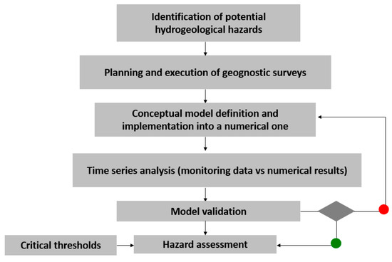
Figure 1.
Framework for hydrogeological risk assessment with dynamic conceptual modeling.
3. Examples of Time Series Analysis in Hydrogeological Modeling Improvement
3.1. Hydrogeological Risk in Tunneling
The hydrogeological risk in tunneling [13,14,15] consists in an inflow risk for the tunnel [16,17], and a water table drawdown with spring depletion for the environment [18,19,20]; these risks can be analyzed by considering, as a performance function, the water balance over a control volume, and the corresponding elements (i.e., rainfall and permeability) can be statistically described, leading to a stochastic modeling approach. Therefore, modeling results can be compared to monitoring data, typically with references to time series of water table drawdown or spring flow rate; for instance, the differences in between the simulated and observed values of water table (residuals) can be analyzed; if differences are detected, specifically an increasing deviation in residuals (purple line in Figure 2), it means that the conceptual model, based on which the numerical one has been implemented, was too simplified. When dealing with hydrogeological problems, a quite typical error consists in considering the presence of a single aquifer, instead of two different aquifers locally interconnected. In such a case, the performance function describing the conceptual model has to be improved for taking into account the two aquifers and their interaction; nevertheless, some parametrical errors could still be present (blue line in Figure 2 exhibits a constant not zero value), and a further calibration of the modeling parameters is still required.
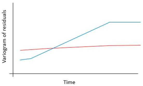
Figure 2.
Deviations between modeling results and observed data obtained by a simplified one-aquifer model (in blue) and a more complex multi-aquifer model (in red).
3.2. Landslide Hydrogeological Risk
The Vajont landslide is a typical example in which several attempts were made to frame and interpret the geological and hydrogeological setting, improving the conceptual model from time to time.
In particular, as far as the hydrogeological conceptual model aimed at describing the “landslide-aquifer-reservoir” is concerned, time series arising from some piezometers of different depths were analyzed and compared to time series of reservoir level and displacements. Based on this comparison, an inconsistency in water table data was detected; in particular, by carrying out an analysis of the linear correlation between the data recorded by piezometers and the reservoir level, one of the piezometers showed data uncorrelated with respect to the others (Figure 3). The first conceptual model, which accounted for a single-layer aquifer, was unable to explain this anomaly; this meant that it contained an error. In fact, it was too simplified for reproducing the real system complexity. Indeed, subsequent studies [21] reconstructed the correct conceptual model, by identifying the existence of a low permeability layer which separates two aquifers: one in the landslide mass and the other one in the underlying bedrock. This updated conceptual model could explain the trend of both shallow and deep piezometers. In fact, the two aquifers had different flow conditions; the shallow one was strongly influenced by the reservoir level (as shown in pz1 and pz3) whereas, in the confined aquifer (pz2), the water table was independent of the reservoir level and strictly correlated to the total rainfall of the previous period [21]. This updated conceptual model allowed the authors to identify a stability threshold for the landslide, as a function of the reservoir level and rainfall in the previous 30 days, related to the measured landslide displacements.
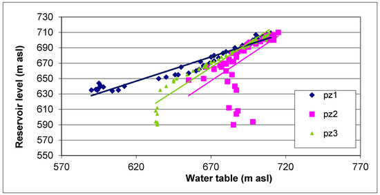
Figure 3.
Statistical correlation between water table in piezometers of different depths (pz1 and pz3 are in the shallow aquifer, whereas pz2 is in the confined one) and the reservoir level.
3.3. Groundwater Pollution Risk
The characterization of groundwater pollution involves the statistical analysis of monitoring data both in time and in space (i.e., multivariate analyses, association and correlation indexes on time series, variogram analyses on special distribute data), and it should lead to the identification of the pollution source and processes, as well as to a description of the groundwater quality and vulnerability.
In more detail, the statistical analysis of monitoring data should concern not only the time evolution of pollution, but also the possible relationships between the different contaminants (Figure 4), as well as the relationships between water table and pollution trends. Indeed, an analysis of correlation can be carried out among the time series of all those variables that are representative of cause–effect phenomena; for example, by comparing the time series of water table with the time series of the concentration of some peculiar pollutants, it is possible to verify whether the latter arises from a release of contaminants stored into an aquitard or in non-saturated soils.
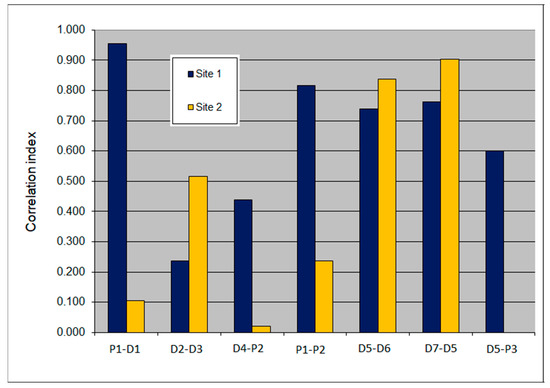
Figure 4.
Correlation indexes between the concentrations of some compounds in different polluted sites: in site 1, primary contaminants (Pi) and their degradation products (Di) are predominant and well correlated; in site 2, the correlation between Pi and Di decreases, which involves a different pollution source (afterwards identified with a dump).
Once the processes involved in the pollution event have been identified, a further analysis can be carried out by using variograms in order to identify not only the most polluted areas and their evolution though time, but the type of contamination, too (hot-spot, plume or diffuse; Figure 5).
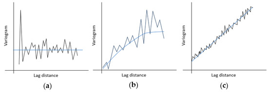
Figure 5.
Variograms corresponding to different types of groundwater pollution: (a) hot spots bring about a nugget effect, such as for the CVM in an industrial site, (b) plume involves a spherical variogram in the groundwater flow direction, such as for chlorides in the same industrial site and (c) diffuse contamination usually shows a linear trend, such as for nitrates in a large-scale alluvial aquifer.
4. Conclusions
Groundwater flow and transport are controlled by physical properties that are characterized by a high degree of heterogeneity and by scales of variation that span several orders of magnitude. This complexity can lead to unexpected risk in many applicative fields, from water resources management to civil engineering design and land planning, and therefore requires a strategy for risk mitigation. With this aim, a statistical analysis of the available data and time series can be used in order to detect possible errors in the hydrogeological conceptual model, thus improving its reliability.
The examples proposed in the present paper show the usefulness of this approach in the applicative field of hydrogeology, as it allows, firstly, the upgrading of the conceptual model of the system and then the subsequent numerical modeling results, especially when the hydrogeological setting is very complex. In fact, this approach quantifies the relevance of the different elements involved in the hydrogeological system and the related processes, therefore identifying errors which can be corrected in order to update the conceptual model.
Funding
This research received no external funding.
Institutional Review Board Statement
Not applicable.
Informed Consent Statement
Not applicable.
Data Availability Statement
Data sharing not applicable.
Conflicts of Interest
The authors declare no conflict of interest.
References
- Boronina, A.; Renard, P.; Balderer, W.; Christodoulides, A. Groundwater resources in the Kouros catchment (Cyprus): Data analysis and numerical modelling. J. Hydrol. 2002, 271, 130–149. [Google Scholar] [CrossRef]
- Francani, V.; Gattinoni, P. Statistical risk analysis of groundwater pollution. In GeoCongress 2008: Geosustainability and Geohazard Mitigation; American Society of Civil Engineers: Reston, VA, USA, 2008; Volume 178, pp. 154–161. [Google Scholar]
- Gattinoni, P. Parametrical landslide modeling for the hydrogeological susceptibility assessment: From the Crati Valley to the Cavallerizzo landslide (Southern Italy). Nat. Hazards 2008, 50, 161–178. [Google Scholar] [CrossRef]
- Loaiciga, H.A.; Charbeneau, R.J.; Everett, L.G.; Fogg, G.E.; Hobbs, B.F.; Rouhani, S. Review of Ground-Water Quality Monitoring Network Design. J. Hydraul. Eng. 1992, 118, 11–37. [Google Scholar] [CrossRef]
- Makropoulos, C.; Koutsoyiannis, D.; Stanić, M.; Djordjević, S.; Prodanović, D.; Dašić, T.; Prohaska, S.; Maksimović, C.; Wheater, H. A multi-model approach to the simulation of large scale karst flows. J. Hydrol. 2008, 348, 412–424. [Google Scholar] [CrossRef]
- Hassan, A.E. A methodology for validating numerical ground water models. Groundwater 2004, 42, 347–362. [Google Scholar] [CrossRef] [PubMed]
- Straface, S. A procedure of Model Validation with a Bayesian Approach. In XXX IAHR Congress—Agora Thessaloniki. Calibration and Validation of 3D Numerical Model; International Association of Hydraulic Engineering and Research: Thessaloniki, Greece, 2003. [Google Scholar]
- Gaganis, P.; Smith, L. A Bayesian Approach to the quantification of the effect of model error on the predictions of groundwater models. Water Resour. Res. 2001, 37, 2309–2322. [Google Scholar] [CrossRef]
- Flavelle, P. A quantitative measure of model validation and its potential use for regulatory purposes. Adv. Water Resour. 1992, 15, 5–13. [Google Scholar] [CrossRef]
- Davis, P.A.; Goodrich, M.T. A Proposed Strategy for the Validation of Ground-Water Flow and Solute Transport Models. In Proceedings from GEOVAL 1990; Swedish Nuclear Power Inspectorate: Stockholm, Sweden, 1990. [Google Scholar]
- Gattinoni, P.; Scesi, L.; Arieni, L.; Canavesi, M.; Zaffaroni, F. A new rating system for hydrogeological risk management along railway infrastructures in Prealpine zone (northern Italy). Innov. Infrastruct. Solutions 2021, 6, 1–14. [Google Scholar] [CrossRef]
- De Finis, E.; Gattinoni, P.; Scesi, L.; Valletta, A. Conceptual and numerical modelling for hydrogeological hazard assessment in the UNESCO site of Castelseprio (northern Italy). In Proceedings of the International Multidisciplinary Scientific GeoConference SGEM 2018, Albena, Bulgaria, 30 June–9 July 2018; Volume 18, pp. 161–176. [Google Scholar]
- Gattinoni, P.; Scesi, L. From hydrogeological hazard identification to risk assessment in tunnelling: An example in northern Italy. In Proceedings of the 20th International Multidisciplinary Scientific GeoConference SGEM, Albena, Bulgaria, 16–25 August 2020; pp. 519–530. [Google Scholar]
- Loew, S. Groundwater hydraulics and environmental impacts of tunnels in crystalline rocks. In Meccanica e Ingegneria delle Rocce; MIR: Torino, Italy, 2002; pp. 201–217. [Google Scholar]
- Molinero, J.; Samper, J.; Juanes, R. Numerical modeling of the transient hydrogeological response produced by tunnel construction in fractured bedrocks. Eng. Geol. 2002, 64, 369–386. [Google Scholar] [CrossRef]
- Celestino, T.B.; Gianbastiani, M.; Bortolucci, A.A. Water inflows in tunnels: Back-analysis and role of different lining systems. In AITES-ITA 2001, Progress in Tunnelling after 2000; Teuscher, P., Colombo, A., Eds.; Pàtron Editore: Bologna, Italy, 2001; Volume 2, pp. 547–554. [Google Scholar]
- Goodman, R.E.; Moye, D.G.; Van Schalkwyk, A.; Javandel, I. Ground water inflow during tunnel driving. Eng. Geol. 1965, 2, 39–56. [Google Scholar]
- Colombo, L.; Gattinoni, P.; Scesi, L. Influence of underground structures and infrastructures on the groundwater level in the urban area of milan, italy. Int. J. Sustain. Dev. Plan. 2017, 12, 176–184. [Google Scholar] [CrossRef]
- Anagnostou, G. The influence of tunnel excavation on the hydraulic head. Int. J. Numer. Anal. Methods Géoméch. 1995, 19, 725–746. [Google Scholar] [CrossRef]
- Dematteis, A.; Kalamaras, G.; Eusebio, A. A systems approach for evaluating springs drawdown due to tunnelling. In AITES-ITA 2001, Progress in Tunnelling after 2000; Teuscher, P., Colombo, A., Eds.; Pàtron Editore: Bologna, Italy, 2001; Volume 1, pp. 257–264. [Google Scholar]
- Hendron, A.J.; Patton, F.D. The Vaiont Slide, A Geotechnical Analysis Based on New Geologic Observations of the Failure Surface; Tech. Rep. GL-85-5; U.S. Army Corps of Engineers: Washington, DC, USA, 1985.


Disclaimer/Publisher’s Note: The statements, opinions and data contained in all publications are solely those of the individual author(s) and contributor(s) and not of MDPI and/or the editor(s). MDPI and/or the editor(s) disclaim responsibility for any injury to people or property resulting from any ideas, methods, instructions or products referred to in the content. |
© 2023 by the author. Licensee MDPI, Basel, Switzerland. This article is an open access article distributed under the terms and conditions of the Creative Commons Attribution (CC BY) license (https://creativecommons.org/licenses/by/4.0/).