Intrinsic Explainable Self-Enforcing Networks Using the ICON-D2-Ensemble Prediction System for Runway Configurations ^†

Abstract

Weather forecasts are indispensable for the decision on the direction of operation of a runway system. Since the forecasts contain uncertainties, additional challenges arise for runway configuration management (RCM). With developments in machine learning, numerous models have been developed to improve forecasts and assist management. In this contribution, an intrinsically explainable Self-Enforcing Network (SEN) is presented as a decision support system for the RCM at Frankfurt Airport.

1. Introduction

Weather forecasts are fundamental to flight safety and management. The functioning of airport-related meteorological services supports decision-making regarding flight routes and planning [1].

Despite the greatest efforts in recent years to improve weather forecasts, the uncertainties that still exist must be considered [2,3]. In addition, new challenges arise from climatic changes, extreme weather conditions, strong wind shear at low altitudes [4,5], lateral boundary perturbations [6], or general hazardous meteorological conditions [7] that require variation or extension of previous models [8,9,10].

The digitalization and increase in, e.g., sensors and satellite imagery, create a large amount of data that is analyzed with various tools (for an overview, see [8]). For example, Key Performance Indicators (KPIs) are recommended to be used as a propensity metric in the preparation of Terminal Aerodrome Forecasts (TAFs) for future weather conditions [1]. Parameters for traffic management initiatives (TMI) under uncertain weather conditions are proposed using an epsilon greedy approach and a Softmax algorithm [2]. For postprocessing models, natural gradient boosting (NGB), quantile random forests (QRF), distributional regression forests (DRF), or Support Vector Quantile Regression (SVQR) are used [11,12].

Advances in machine learning and deep learning have led to many methods being developed in recent years to improve weather forecasts and support air traffic management (ATM) [13]. These methods are correspondingly diverse, such as an encoder-decoder U-net neural network to forecast convective storms and lightning [10], offline model-free reinforcement learning, or eXtreme Gradient Boosting (XGBoost), to support runway configuration management (RCM) [14,15], detection of adverse weather with EEG-enabled Bayesian neural networks [7], or anomaly detection and hierarchical clustering to spot anomalous data and group similar forecasts [1]. Additional methods are used, e.g., Transductive Long Short Term Memory (T-LSTM) for weather forecasting [16] or Spatio-Temporal Graph Convolutional Network to estimate the arrival and departure capacity under weather impact [17].

Hybrid systems combine different methods and learning concepts, such as supervised, unsupervised, and self-attention [18,19], or decomposition methods with adaptive learning strategies [20].

In comparison, few articles were found in which self-organizing neural networks are used for weather prediction, e.g., structural self-organizing maps (S-SOMs) for weather typing [21], combining SOM with ensemble climate forecasts to investigate the predictability of European summer climate in relation to the North Atlantic jet stream [22], to predict ocean currents [23], or to analyze radar data for nowcasting [24].

A big challenge remains regarding the explainability of the results in the context of ATM [5,25,26,27]. According to Degas et al. [28], the problem for responsible end users in ATM is that the results are difficult to understand or are not transparent for safety-critical areas such as air traffic. Explainability is necessary to (a) describe the algorithms or the results (descriptive xAI), (b) predict the behavior of an algorithm (predictive xAI), or (c) detect errors or undesirable behavior of an AI method (prescriptive xAI).

Explainable AI algorithms are distinguished by their scope. The scope describes the area to which the explanation refers. It can refer to the logic of the entire model (global xAI) or to the explanation of the background of a particular decision (local xAI) [29].

A further differentiation is made between post-hoc and ante-hoc explanation methods. In a post-hoc method, an explanation is given after training, in an ante-hoc method, it is given during training and is already available through the design of the algorithm. This method is also called intrinsic xAI, which is model-specific and explainable due to its internal structure. The learning process is transparent (algorithmic transparency), the technical operation is understandable (simulatability), or the algorithm can be decomposed into its individual parts (decomposability) [30].

We address the problem by showing how decision support for runway selection based on weather forecasts is accomplished with a Self-Enforcing Network (SEN), a self-organized learning neural network [31]. To explain the recommendations, Shapley Values are used to indicate which wind speeds and directions are determinants for the recommendation. Due to the way the overall system works, we are referring to an intrinsically explainable SEN.

The contribution is organized as follows: the next section provides a brief introduction to the methods used. Subsequently, the model as well as the results are presented. Finally, the challenges posed by the new, more complex, and detailed data structure are pointed out, and solution concepts are proposed.

2. Methods

The ensemble forecast system COSMO-DE-EPS, the Self-Enforcing Network (SEN), and Feature Importance using Shapley Values (SV) are briefly described below.

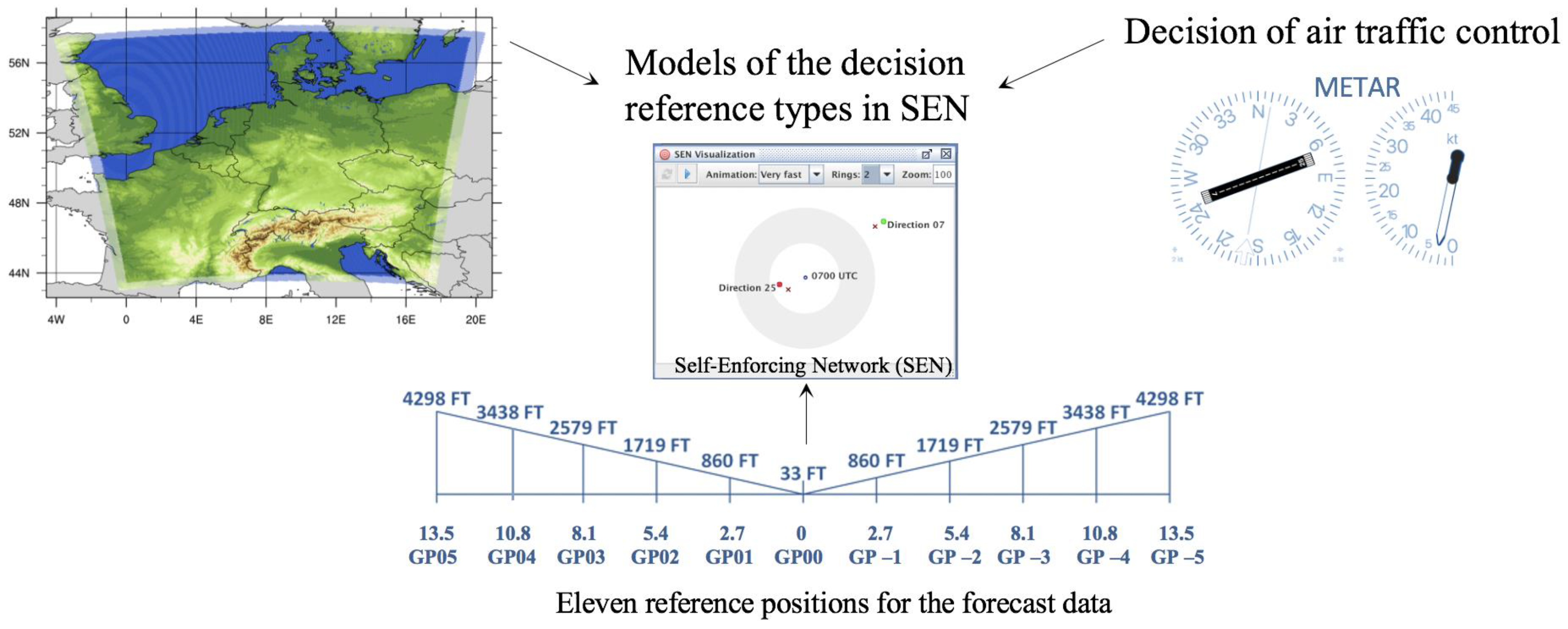
2.1. ICON-D2-EPS

Air traffic management at Frankfurt Airport requires not only weather data for a specific point in time but also forecast data for the next period. The forecast data comes from the ICON-D2 ensemble prediction forecast system (ICON-D2-EPS), which is operated by the German Weather Service (DWD). The use of an ensemble forecast system makes it possible to quantify uncertainties or probabilities for the predicted wind situations.

The main purpose of running an ensemble system is to enable an estimation of the forecast uncertainty, in our case, the development of the wind situation, by running a number of physically consistent scenarios of future development. The different scenarios arise from uncertainties in the initial conditions and model errors. An additional source of forecast uncertainty arises from the border conditions of a limited area model [32].

ICON-D2-EPS is a limited area model and currently consists of 20 ensemble members. It runs eight times a day with 48 h of forecasts for the 00, 03, 06, 09, 12, 15, 18, and 21 UTC runs.

In the case of ICON-D2-EPS, the 20 ensemble members were created through perturbations of the initial state and perturbations of a number of parametrizations of the model physics (e.g., turbulence, microphysics, or shallow convection). In addition, the boundary conditions were received from the global ICON-EPS forecast model, which consists of 40 ensemble members. From the total 40 ensemble members, the first 20 (arbitrarily chosen) were used to provide the boundary conditions for the 20 ensemble members of the limited area model ICON-D2-EPS [32].

On the one hand, this is an advantage over the use of traditional deterministic forecast models, but on the other hand, it poses an additional challenge for management as uncertainty must be included in the decision-making process [33].

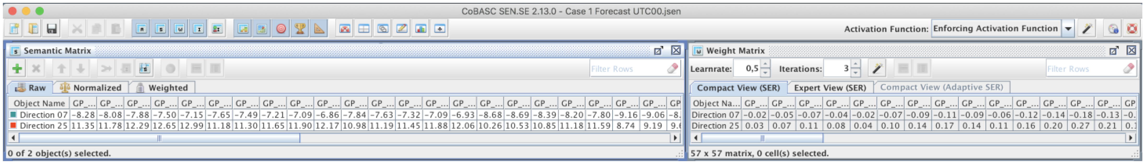
2.2. Self-Enforcing Network (SEN)

The Self-Enforcing Network (SEN) is a deterministic, two-layered, and self-organized learning neural network that acquires and orders knowledge according to cognitive theory learning models [34,35].

The characteristic features of the SEN algorithm and SEN tool are: (a) a semantic matrix; (b) the so-called cue validity factor (cvf) for highlighting essential attributes; (c) the transformation of the data from the semantic matrix into the weight matrix by the specific learning rule; and (d) various visualizations.

(a) The semantic matrix is the basis of the learning process. It contains the essential attributes (features) and their degree of membership in an object [35]. The data is normalized in the interval (−1, 1).

(b) For each feature, a cue validity factor (cvf) is set when building the model. The cue validity factor influences the strength of an attribute’s effect on activation by the network. In the model, the cvf influences how much of the wind from the eleven measurement points is used for the decision. The measurement points that are farthest away have the lowest cvf; beyond that, the middle quantile (median) has the highest cvf (see below, Section 3).

(c) The Self-Enforcing Rule (SER) is the learning rule used in SEN, which transforms the values of the semantic matrix v_sm into a weight value between attribute and object w_ao with the learning rate c, a parameter responsible for adjusting weights in a neural network, and the cue validity factor (cvf_a):

$$w_{ao}=c\times v_{sm}\times {cvf}_a.$$

(1)

The peculiarity of SEN is that the weight matrix is not randomly generated.

There are several activation functions available that return the activation value a_j of a neuron; for this problem, the enforcing activation function (EAF) is the most suitable [33]. In the general representation of the functions in neural networks, w_ij (the weight w between the sending neuron i and the receiving neuron j) is the equivalent of w_ao:

$$a_j=\sum _{i=1}^n\frac{w_{ij}\times a_i}{1+|w_{ij}\times a_i|}.$$

(2)

(d) The following visualizations are used to display the results: The so-called map visualization places the reference types on a two-dimensional map. The greater the Euclidean distance between the objects, the further apart they are shown on the map; correspondingly, similar objects are close together.

In the SEN-visualization, the activation values indicate the degree of similarity between the new input data (weather forecasts) and the reference types, i.e., the runway directions. The higher the final activation values are, the more the input data resembles the reference types. The computed Euclidean distances are also displayed, where similarity is indicated by the smallest distance between the input data and the reference types (see below, Section 3).

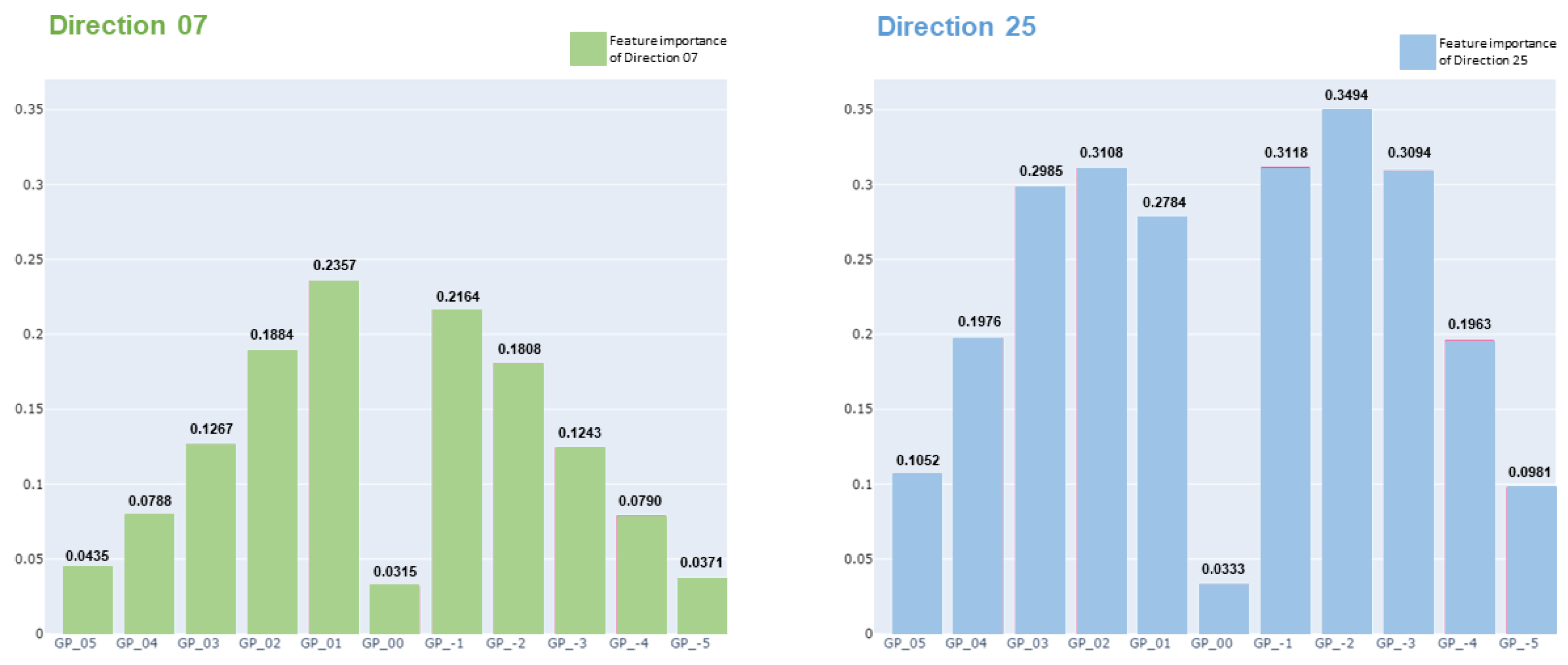
2.3. Shapley Values

The calculation of the Feature Importance is based on the concept of Shapley Values (SV) from the cooperative game theory of Shapley [36], according to which the influence of a player can be computed considering the effects of cooperation and individual performance on the game outcome.

The value a player contributes to the payoff is called the SV, with four defining properties: “zero player property”, “efficiency”, “symmetry”, and “linearity” [37].

The zero player property means that an actor receives no share of the payoff if that actor contributes nothing to the final outcome. The efficiency property refers to the actual influence of an actor on the outcome and allows inferences to be made about that actor. Symmetry states that two actors who have the same influence on the outcome have the same SV. Apart from that, the actor who contributes the most has the highest SV. Linearity ensures that the sum of all SVs accounts for the total influence on the outcome.

Only if these four properties are true can a value be called a Shapley Value. The SV Φ of a player i on the game outcome v can be calculated with the following formula [38]:

$${\Phi }_i\left(v\right)=\sum _{S\subseteq N\setminus \left\{i\right\}}\frac{\left|S\right|!\left(n-1-\left|S\right|\right)!}{n!}\left(v\left(S\cup \left\{i\right\}\right)-v\left(S\right)\right).$$

(3)

From the set of players participating in the game, all possible player sets S are formed, each containing a subset n of the entire number of players N. The influence Φ of player i on the outcome of the game v is calculated for each player set, considering the effects of cooperation between the players. The total contribution of the player to the game outcome Φ_i(v) is the sum of all partial influences resulting from coalitions in the respective player sets.

It turns out that the features in SEN have the properties of dummy players [39]. Dummy players are SV whose constant contribution to the game result is independent of the other players.

This property results from the fact that the weight matrix is not initialized with random values but with the values from the semantic matrix. This leads to the effect that the weight values directly reflect the importance of the individual attributes in the reference types, and thus the SV has corresponding effects on the output. Therefore, the formula for calculating the SV is shortened to [39]:

$${\Phi }_i\left(v\right)=v\left(i\right).$$

(4)

The four properties of Shapley Values described above are met since, on the one hand, the feature’s individual impact on the total activation is extracted, and on the other hand, the added values constitute the total activation value.

Because of the structure and operation of SEN and the immediate identification of its Feature Importance, we can consider SEN to be an intrinsically Explainable AI.

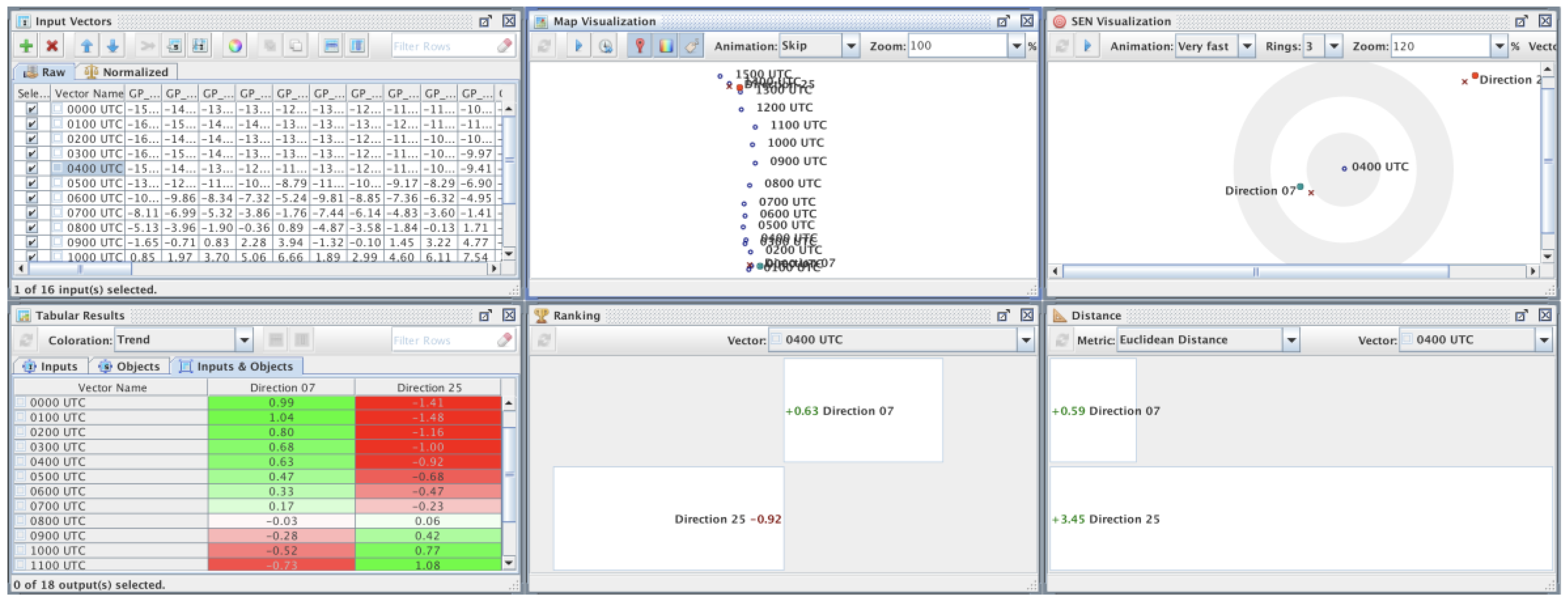
3. Model and Results

The operating direction of the runway system has to be selected according to the wind conditions between the ground and up to approximately 5000 m. The two possible operating directions at Frankfurt airport are “Direction 07”, used during generally easterly winds, and “Direction 25”, used during westerly winds.

The weather data necessary for the appropriate decisions are derived from the COSMO-DE-EPS ensemble prediction System of the German Weather Service (Deutscher Wetterdienst (DWD)).

The required weather data are ensemble forecasts for 11 reference positions located at different distances along the glide path to the airport and on the airport itself. For each position, five quantiles (i.e., a statistical measure reflecting the dispersion of the ensemble forecasts) are computed for the parallel wind component (i.e., the headwind or tailwind component of a departing or approaching aircraft). The ensemble forecast data of the DWD, processed over years, are the basis for our experiments.

For the development of the reference types, representing the operation directions 07 and 25 at the airport in Frankfurt, the decisions of air traffic controllers based on the weather forecasts were considered. The knowledge of several experts (including meteorologists, air traffic controllers, and SEN developers) was incorporated into the development of the model shown in Figure 1.

The reference types for directions 07 and 25 are defined in the semantic matrix, which contains 55 attributes (5 wind components reflecting the 5 quantiles for each of the 11 measurement points of the forecasted wind direction at the reference positions along the glide path—GP). The normalized data are transformed into the weight matrix using the learning rule and are learned by SEN as “representative or ideal wind conditions” with a learning rate c of 0.5 and three iterations using the Enforcing Activation Function (EAF). In Figure 2, there is a section of the reference types in which the west direction always contains negative values [35].

After the learning process and given new input data (weather forecasts), different visualizations are available, as shown in Figure 3 with a recent weather forecast.

The input vectors include the forecasted data at 0000 UTC for the next fifteen hours. The two visualizations next to the input vectors show the similarity of the forecasts to the reference types for the corresponding operation direction. In the SEN visualization, only one selected prediction is focused, and the appropriate reference type is attracted according to the similarity of the wind conditions. In the map visualization, all predictions are classified into the reference types Direction 07 (at the bottom) and Direction 25 (at the top). The calculated activation values are visualized in tabular form (colored green for high positive activation, white for low activation and red for high negative activation) as well as by bars sorted according to highest activation (Ranking) and smallest Euclidean distance (Distance). In this case, the unambiguous recommendation is runway 07.

The intrinsic explainability of SEN allows the straightforward determination and visualization of the feature’s importance for the final activation of a forecast. For a better interpretation of the results, it was decided to calculate the feature importance for the 11 measurement points along the glide path and to adjust the visualization by rotating the visualization by 90 degrees and sorting the values according to the location on the glide path. Figure 4 shows the feature importance of the two reference types, Directions 07 (colored green) and Direction 25 (colored blue).

The forecast at 0000 UTC for 0400 UTC is classified by SEN as Direction 07 with a final activation of 0.63 (Figure 3). An analysis of the feature importance of this prediction in Figure 5 shows the influence of the conditions at the measurement points on the final activation compared to the classified direction. For 0400 UTC, the high-altitude winds (GP_5, GP_4) have a stronger influence on the final result than for Direction 07, while the medium-altitude winds at GP_3, GP_2, and GP_1 have a weaker influence. The winds directly on the runway (GP_00) have a negative Feature Importance. Here, wind conditions oppose the use of Direction 07 and thus support the use of Direction 25 by reducing the activation of Direction 07.

The prediction at 0000 UTC (Figure 3) can be further analyzed by examining the change in feature importance at the fifteen predicted times (Figure 6).

The influence of the high-altitude winds decreases in the course of time until 0700 UTC, and the ground-level wind has less and less influence on the final activation, too. At 0800 UTC, the winds are classified by SEN as being in direction 25, and thus a change of the operating direction is recommended. Here the correspondence between ranking and distances is not correct, an indication of the upcoming change (Figure 7). Currently, the winds close to the ground are crucial for the decision. Until 1400 UTC, the feature importance increases at all measurement points, and finally, even the high-altitude winds have a stronger activation than the classified direction 25.

The forecast at 0000 UTC predicts a change of direction from Direction 07 to Direction 25 at 0800 UTC. Examining the forecasts between 1800 UTC of the previous day and 0900 UTC of the following day, the change was already predicted at that time. Figure 8 shows the map visualization of SEN for the different forecasts, which was created in Python. This visualization was not generated by attraction and repulsion as in the SEN tool but by calculating the concrete coordinates; nevertheless, it gives the same representation. The line between the forecasts allows the user to see the progression of the forecast. The corridor immediately indicates the time at which a change in wind direction occurs.

Upon analyzing the Feature Importance at the time of the change, it can be seen how the recommendation for a change at 0800 UTC strengthened over time as the time of the change got closer (Figure 9).

In this case, at 0249 UTC, it was decided to start air traffic with Direction 25 at the start of flight operations at 0400 UTC. This was justifiable because, until 0800 UTC, the winds were very weak, and in this case, flight operations with a tailwind were possible. This saved the costly change during the day.

4. Conclusions and Recent Work

For complex systems such as weather forecasting and runway configuration management, we have shown how Feature Importance can be used to help understand the results of the recommendation. The architecture and learning procedures of SEN fulfill the properties of Shapley Values with no loss of performance in determining Feature Importance. Feature Importance can be read directly by decomposing a vector into its individual components; thus, SEN can be classified as intrinsically Explainable AI.

While the first version used for predicting the best runway to approach used 11 selected measurement points in the planes’ glide path, a currently enhanced model utilizes wind data from around the airport in an area of 2.500 km². When taking into account the area, the grid’s density, and the number of ensembles, this increases the amount of input data to be processed for a single prediction by a factor of more than 168.000. With thousands of available training data entries, the amount of data to be processed is staggering. The fact that weight matrices grow exponentially with increasing object numbers complicates matters even further.

The amount of data to deal with has two consequences: firstly, raw data can no longer be inspected reasonably because the human mind is unable to cope with the given amount. Secondly, the required computational power to run experiments is not available on current consumer desktop systems. This applies especially to the number of CPU cores available.

The above considerations lead to the following consequences:

• It is necessary to build tools to view raw data in an aggregated and easily perceivable manner.
• It is necessary to move the experimentation software away from a desktop application and towards a command-line tool that can be executed on a HPC. Techniques and optimizations have to be introduced to deal with the new dimension of data.
• The modeling process can no longer be accomplished by a human alone but instead needs to be computer-aided in terms of data selection for the training process and validation of the resulting model.
• When discussing the results with domain experts, i.e., air traffic controllers, the decisions taken by the system must be retraceable and must be presented to them in a manner that makes it clear how the predicted result came about.

We are confident that the usage of Explainable AI, as presented in this contribution, will support the professional exchange with flight controllers by enabling us to quickly comprehend why the system came to a specific prediction and which edge cases can be ignored or must be considered.

References

- Patriarca, R.; Simone, F.; Di Gravio, G. Supporting weather forecasting performance management at aerodromes through anomaly detection and hierarchical clustering. Expert Syst. Appl. 2023, 213, 119210. [Google Scholar] [CrossRef]
- Jones, J.C.; Ellenbogen, Z.; Glina, Y. Recommending strategic air traffic management initiatives in convective weather. J. Air Transp. 2023, 31, 45–56. [Google Scholar] [CrossRef]
- Scala, P.; Mota, M.M.; Ma, J.; Delahaye, D. Tackling uncertainty for the development of efficient decision support system in air traffic management. IEEE Trans. Intell. Transp. Syst. 2019, 21, 3233–3246. [Google Scholar] [CrossRef]
- Bombelli, A.; Sallan, J.M. Analysis of the effect of extreme weather on the US domestic air network. A delay and cancellation propagation network approach. J. Transp. Geogr. 2023, 107, 103541. [Google Scholar] [CrossRef]
- Khattak, A.; Chan, P.-W.; Chen, F.; Peng, H. Prediction of a Pilot’s Invisible Foe: The Severe Low-Level Wind Shear. Atmosphere 2023, 14, 37. [Google Scholar] [CrossRef]
- Zhang, L.; Min, J.; Zhuang, X.; Wang, S.; Qiao, X. The Lateral Boundary Perturbations Growth and Their Dependence on the Forcing Types of Severe Convection in Convection-Allowing Ensemble Forecasts. Atmosphere 2023, 14, 176. [Google Scholar] [CrossRef]
- Yiu, C.Y.; Ng, K.K.H.; Li, X.; Zhang, X.; Li, Q.; Lam, H.S.; Chong, M.H. Towards safe and collaborative aerodrome operations: Assessing shared situational awareness for adverse weather detection with EEG-enabled Bayesian neural networks. Adv. Eng. Inform. 2022, 53, 101698. [Google Scholar] [CrossRef]
- Fathi, M.; Haghi Kashani, M.; Jameii, S.M.; Mahdipour, E. Big Data Analytics in Weather Forecasting: A Systematic Review. Arch. Comput. Methods Eng. 2022, 29, 1247–1275. [Google Scholar] [CrossRef]
- Gonzalo, J.; Domínguez, D.; López, D.; García-Gutiérrez, A. An analysis and enhanced proposal of atmospheric boundary layer wind modelling techniques for automation of air traffic management. Chin. J. Aeronaut. 2021, 34, 129–144. [Google Scholar] [CrossRef]
- Li, Y.; Liu, Y.; Sun, R.; Guo, F.; Xu, X.; Xu, H. Convective Storm VIL and Lightning Nowcasting Using Satellite and Weather Radar Measurements Based on Multi-Task Learning Models. Adv. Atmos. Sci. 2023, 40, 887–899. [Google Scholar] [CrossRef]
- Benáček, P.; Farda, A.; Štěpánek, P. Postprocessing of Ensemble Weather Forecast Using Decision Tree–Based Probabilistic Forecasting Methods. Weather Forecast. 2023, 38, 69–82. [Google Scholar] [CrossRef]
- Takamatsu, T.; Ohtake, H.; Oozeki, T. Support Vector Quantile Regression for the Post-Processing of Meso-Scale Ensemble Prediction System Data in the Kanto Region: Solar Power Forecast Reducing Overestimation. Energies 2022, 15, 1330. [Google Scholar] [CrossRef]
- Tang, J.; Liu, G.; Pan, Q. Review on artificial intelligence techniques for improving representative air traffic management capability. J. Syst. Eng. Electron. 2022, 33, 1123–1134. [Google Scholar] [CrossRef]
- Churchill, A.; Coupe, W.J.; Jung, Y.C. Predicting Arrival and Departure Runway Assignments with Machine Learning. In Proceedings of the 2021 AIAA AVIATION FORUM, Virtual, 2–6 August 2021. [Google Scholar] [CrossRef]
- Memarzadeh, M.; Puranik, T.G.; Battistini, J.; Kalyanam, K.M.; Ryan, W. Airport Runway Configuration Management with Offline Model-Free Reinforcement Learning. In Proceedings of the 2023 AIAA SCITECH Forum, National Harbor, MD, USA, 23–27 January 2023. [Google Scholar] [CrossRef]
- Venkatachalam, K.; Trojovský, P.; Pamucar, D.; Bacanin, N.; Simic, V. DWFH. An improved data-driven deep weather forecasting hybrid model using Transductive Long Short Term Memory (T-LSTM). Expert Syst. Appl. 2023, 213, 119270. [Google Scholar] [CrossRef]
- Tang, S.; Fang, Q.; Yang, Y.; Chen, J.; Cai, K. A Learning Estimation Approach for Arrival and Departure Capacity considering Weather Impact. In Proceedings of the 2022 IEEE/AIAA 41st Digital Avionics Systems Conference (DASC), Portsmouth, VA, USA, 18–22 September 2022. [Google Scholar] [CrossRef]
- Ren, X.; Li, X.; Ren, K.; Song, J.; Xu, Z.; Deng, K.; Wang, X. Deep Learning-Based Weather Prediction: A Survey. Big Data Res. 2021, 23, 100178. [Google Scholar] [CrossRef]
- Schultz, M.G.; Betancourt, C.; Gong, B.; Kleinert, F.; Langguth, M.; Leufen, L.H.; Mozaffari, A.; Stadtler, S. Can deep learning beat numerical weather prediction? Philos. Trans. R. Soc. A 2021, 379, 20200097. [Google Scholar] [CrossRef]
- Zouaidia, K.; Rais, M.S.; Ghanemi, S. Weather forecasting based on hybrid decomposition methods and adaptive deep learning strategy. Neural Comput. Appl. 2023, 35, 11109–11124. [Google Scholar] [CrossRef]
- Doan, Q.-V.; Kusaka, H.; Sato, T.; Chen, F. S-SOM v1. 0: A structural self-organizing map algorithm for weather typing. Geosci. Model Dev. 2021, 14, 2097–2111. [Google Scholar] [CrossRef]
- Carvalho-Oliveira, J.; Borchert, L.F.; Zorita, E.; Baehr, J. Self-organizing maps identify windows of opportunity for seasonal European summer predictions. Front. Clim. 2022, 4, 844634. [Google Scholar] [CrossRef]
- Vilibić, I.; Šepić, J.; Mihanović, H.; Kalinić, H.; Cosoli, S.; Janeković, I.; Žagar, N.; Jesenko, B.; Tudor, M.; Dadić, V.; et al. Self-Organizing Maps-based ocean currents forecasting system. Sci. Rep. 2016, 6, 22924. [Google Scholar] [CrossRef]
- Czibula, G.; Mihai, A.; Mihuleţ, E.; Teodorovici, D. Using self-organizing maps for unsupervised analysis of radar data for nowcasting purposes. Procedia Comput. Sci. 2019, 159, 48–57. [Google Scholar] [CrossRef]
- Midtfjord, A.D.; De Bin, R.; Huseby, A.B. A decision support system for safer airplane landings: Predicting runway conditions using XGBoost and explainable AI. Cold Reg. Sci. Technol. 2022, 199, 103556. [Google Scholar] [CrossRef]
- Rudd, K.; Eshow, M.; Gibbs, M. Method for Generating Explainable Deep Learning Models in the Context of Air Traffic Management. In Proceedings of the Machine Learning, Optimization, and Data Science: 7th International Conference, LOD 2021, Grasmere, UK, 4–8 October 2021. Revised Selected Papers, Part I; 2022. [Google Scholar] [CrossRef]
- Xie, Y.; Pongsakornsathien, N.; Gardi, A.; Sabatini, R. Explanation of machine-learning solutions in air-traffic management. Aerospace 2021, 8, 224. [Google Scholar] [CrossRef]
- Degas, A.; Islam, M.R.; Hurter, C.; Barua, S.; Rahman, H.; Poudel, M.; Ruscio, D.; Ahmed, M.U.; Begum, S.; Rahman, A.; et al. A survey on artificial intelligence (ai) and explainable ai in air traffic management: Current trends and development with future research trajectory. Appl. Sci. 2022, 12, 1295. [Google Scholar] [CrossRef]
- Schwalbe, G.; Finzel, B. A comprehensive taxonomy for explainable artificial intelligence: A systematic survey of surveys on methods and concepts. Data Min. Knowl. Discov. 2023. [Google Scholar] [CrossRef]
- Arrieta, A.B.; Díaz-Rodríguez, N.; Del Ser, J.; Bennetot, A.; Tabik, S.; Barbado, A.; García, S.; Gil-Lopez, S.; Molina, D.; Benjamins, R.; et al. Explainable Artificial Intelligence (XAI): Concepts, taxonomies, opportunities and challenges toward responsible AI. Inf. Fusion 2020, 58, 82–115. [Google Scholar] [CrossRef]
- Greisbach, A.; Klüver, C. Determining Feature Importance in Self-Enforcing Networks to achieve Explainable AI (xAI). In Proceedings 32. Workshop Computational Intelligence; Schulte, H., Hoffmann, F., Mikut, R., Eds.; KIT Scientific Publishing: Karlsruhe, Germany, 2022; pp. 237–256. [Google Scholar]
- Reinert, D.; Prill, F.; Frank, H.; Denhard, M.; Baldauf, M.; Schraff, C.; Gebhardt, C.; Marsigli, C.; Zängl, G. DWD Database Reference for the Global and Regional ICON and ICON-EPS Forecasting System. 2023. Available online: https://www.dwd.de/SharedDocs/downloads/DE/modelldokumentationen/nwv/icon_d2/icon_d2_dbbeschr_aktuell.pdf?view=nasPublication&nn=13934 (accessed on 27 June 2023).
- Klüver, C.; Klüver, J.; Zinkhan, D. A self-enforcing neural network as decision support system for air traffic control based on probabilistic weather forecasts. In Proceedings of the IEEE International Joint Conference on Neural Networks (IJCNN), Anchorage, AK, USA, 14–19 May 2017; pp. 729–736. [Google Scholar] [CrossRef]
- Klüver, C.; Klüver, J. Self-organized learning by self-enforcing networks. In IWANN 2013, LNCS 7902; Part I; Rojas, I., Joya, G., Cabestany, J., Eds.; Springer: Berlin/Heidelberg, Germany, 2013; pp. 518–529. [Google Scholar] [CrossRef]
- Zinkhan, D.; Eiermann, S.; Klüver, C.; Klüver, J. Decision Support Systems for Air Traffic Control with Self-enforcing Networks Based on Weather Forecast and Reference Types for the Direction of Operation. In Advances in Computational Intelligence; IWANN 2021. Lecture Notes in Computer Science; Rojas, I., Joya, G., Catala, A., Eds.; Springer: Cham, Switzerland, 2021; Volume 12862, pp. 404–415. [Google Scholar] [CrossRef]
- Shapley, L.S. A Value for n-Person Games. In Contributions to the Theory of Games (AM-28); Kuhn, H.W., Tucker, A.W., Eds.; Princeton University Press: Princeton, NJ, USA, 1953; Volume 2, pp. 307–318. [Google Scholar]
- Rozemberczki, B.; Watson, L.; Bayer, P.; Yang, H.-T.; Kiss, O.; Nilsson, S.; Sarkar, R. The shapley value in machine learning. arXiv 2022, arXiv:2202.05594. [Google Scholar]
- Bokati, L.; Kosheleva, O.; Kreinovich, V.; Thach, N.N. Why Shapley Value and Its Variants Are Useful in Machine Learning (and in Other Applications). Proc., 15. Workshop Computational Intelligence. Departmental Technical Reports (CS). 1729. 2022. Available online: https://scholarworks.utep.edu/cs_techrep/1729/ (accessed on 27 June 2023).
- Casajus, A.; Huettner, F. Null, nullifying, or dummifying players: The difference between the Shapley value, the equal division value, and the equal surplus division value. Econ. Lett. 2014, 122, 167–169. [Google Scholar] [CrossRef]
Disclaimer/Publisher’s Note: The statements, opinions and data contained in all publications are solely those of the individual author(s) and contributor(s) and not of MDPI and/or the editor(s). MDPI and/or the editor(s) disclaim responsibility for any injury to people or property resulting from any ideas, methods, instructions or products referred to in the content. |
© 2023 by the authors. Licensee MDPI, Basel, Switzerland. This article is an open access article distributed under the terms and conditions of the Creative Commons Attribution (CC BY) license (https://creativecommons.org/licenses/by/4.0/).
Share and Cite
Zinkhan, D.; Greisbach, A.; Zurmaar, B.; Klüver, C.; Klüver, J. Intrinsic Explainable Self-Enforcing Networks Using the ICON-D2-Ensemble Prediction System for Runway Configurations. Eng. Proc. 2023, 39, 41. https://doi.org/10.3390/engproc2023039041
Zinkhan D, Greisbach A, Zurmaar B, Klüver C, Klüver J. Intrinsic Explainable Self-Enforcing Networks Using the ICON-D2-Ensemble Prediction System for Runway Configurations. Engineering Proceedings. 2023; 39(1):41. https://doi.org/10.3390/engproc2023039041
Chicago/Turabian StyleZinkhan, Dirk, Anneliesa Greisbach, Björn Zurmaar, Christina Klüver, and Jürgen Klüver. 2023. "Intrinsic Explainable Self-Enforcing Networks Using the ICON-D2-Ensemble Prediction System for Runway Configurations" Engineering Proceedings 39, no. 1: 41. https://doi.org/10.3390/engproc2023039041
APA StyleZinkhan, D., Greisbach, A., Zurmaar, B., Klüver, C., & Klüver, J. (2023). Intrinsic Explainable Self-Enforcing Networks Using the ICON-D2-Ensemble Prediction System for Runway Configurations. Engineering Proceedings, 39(1), 41. https://doi.org/10.3390/engproc2023039041