A Forecasting Model for the Prediction of System Imbalance in the Greek Power System ^†

Abstract

Forecasting imbalance volumes are of great importance for the different actors in electricity markets. From a transmission system operator (TSO) perspective, balancing supply and demand in real-time is one of the main operational tasks to ensure the safe and reliable operation of the power system, while market participants also use forecasting tools to enhance their participation strategy in electricity wholesale markets. Over the last few years, the increasing integration of renewable energy sources into the power system has created additional complexity for the problem of accurately determining the imbalance volume. In the present work, a case study of the Greek balancing market is presented and analysed. Different algorithms and a set of external predictors are adopted both from the market and operational perspective and compared for two different forecasting horizons.

1. Introduction

Over the last several years, the increasing penetration of renewable generation into the energy mix has significantly changed system operations. The intermittency introduced in the system creates more frequent deviations between supply and demand, which are defined as system imbalances. In power systems, system imbalances can occur due to a number of factors, including fluctuations in demand and supply, generation outages, transmission constraints and strategic bidding. Demand fluctuations can be caused either by seasonal changes and weather conditions or by load operational constraints, while supply fluctuations are mostly due to generation constraints and commercial considerations, and, recently, due to the volatility in weather-dependent, energy-limited power sources (e.g., wind, solar, etc.). Generation outages of dispatchable power sources can also be a great source of system imbalances since they usually cover a considerable part of system demand. An indicative recent example came from France in 2022, in which the unscheduled nuclear power plant outages caused imbalances not only in the French network, but also in neighbouring countries (e.g., Belgium), due to the interconnection between the neighboring countries [1].

Finally, the transmission constraints constitute a structural—yet important—limitation of the power system. For example, if there is an over-generation situation in one region but the transmission lines are congested or at capacity, the excess energy may not be able to be transferred to another region where the demand is high. The over-generation disrupts the net position of the local area, which ideally should be kept constant. This can lead to an over-generation situation in one region and an under-generation situation in another, causing local imbalances. System operators are responsible for alleviating this problem in the spot energy markets by mainly redispatching generation to where it is needed, which is a decision that is economically not optimal and creates security challenges in some cases. Recently, measures such as dispatching economic demand response programs (managing electricity demand), and using storage plants, either as standalone systems or in combination with renewable assets (i.e., in hybrid configurations), have also been applied. In the longer timeframe, imbalances due to grid constraints can be managed by investing in transmission system upgrades (increasing the system capacity). For example, in Greece, the transmission system operator (TSO) has massively invested in transmission grid upgrades in order to increase its capacity and improve system reliability; significant RES developments are expected to be integrated into the network in forthcoming years [2].

In this paper, we propose a new methodology for predicting power system imbalances, a key factor in system reliability and energy market mechanics. The literature in the field is limited and only a few relevant publications can be found, in contrast to those addressing classical problems of load [3], RES [4] and DAM price forecast [5,6]. Nevertheless, the problem has started to attract increasing attention in the last few years, mostly due to the massive penetration of green energy technologies into the grid. Elia, the Belgian TSO, has recently published a methodology for the deterministic and probabilistic prediction of system imbalance [7]. The deterministic model is a standard linear regression with external predictors, while the probabilistic model is implemented using binomial logistic regression. A forecast is then produced and updated on a minute basis for the current and the following quarter-hour. In [8], one of the first studies in the field of system imbalance forecasting was presented, focusing on statistical techniques for the prediction process. Classical time series models (e.g., ARIMA, exponential smoothing) were employed. The presented results were of mixed promise, mainly due to the non-stationarity of the balancing data and short-term operational issues, and possibly also due to energy market conditions, such as market strategic bidding. Furthermore, [8] employed a novel data-mining technique to showcase the additional benefits when combined with classical algorithms. In [9], the most important predictors for the prediction of system imbalance in the Czech power system were presented. The predictors were divided into demand and supply variables, while the behavior of the market participants was also modelled. The results of the proposed model were compared to an ARIMA benchmark model. In [10], a random forest regressor for the prediction of the Spanish system’s imbalance was presented. The analysis highlighted the benefits of an ensembling technique for system imbalance prediction, but the limited period for data analysis should also be noted. Finally, the study presented in [11] is particularly relevant as intra-hour forecasting was developed for the case of the Norwegian TSO, Statnett. The imbalance forecasting tool developed relies on quantile regression forests producing probabilistic outputs. The tool was compared to the business-as-usual approach of TSO (Planning Table) and provided significant enhancements. Apart from some theoretical analysis for the Greek case that can be found in [12,13], in which the current status and future challenges of the market are addressed, to the best of our knowledge, this work is the first that deals directly with the prediction of system imbalance in the Greek market. In [14], an approach for the probabilistic dimensioning of frequency restoration reserves was developed and compared to static dimensioning of the Greek electricity market. The main purpose of this paper is to develop a forecasting methodology for the accurate prediction of system imbalance leading to improved system reliability, decreased energy procurement costs and optimal activation of the balancing reserves.

This paper is organized as follows: In Section 2, a short description of the Greek electricity market is provided, while in Section 3, the proposed methodology is presented. In Section 4, a statistical analysis focusing on data from the Greek case study is conducted and the results obtained are given in Section 5. Finally, in Section 6, some useful conclusions are drawn, focusing on comparison of the different models.

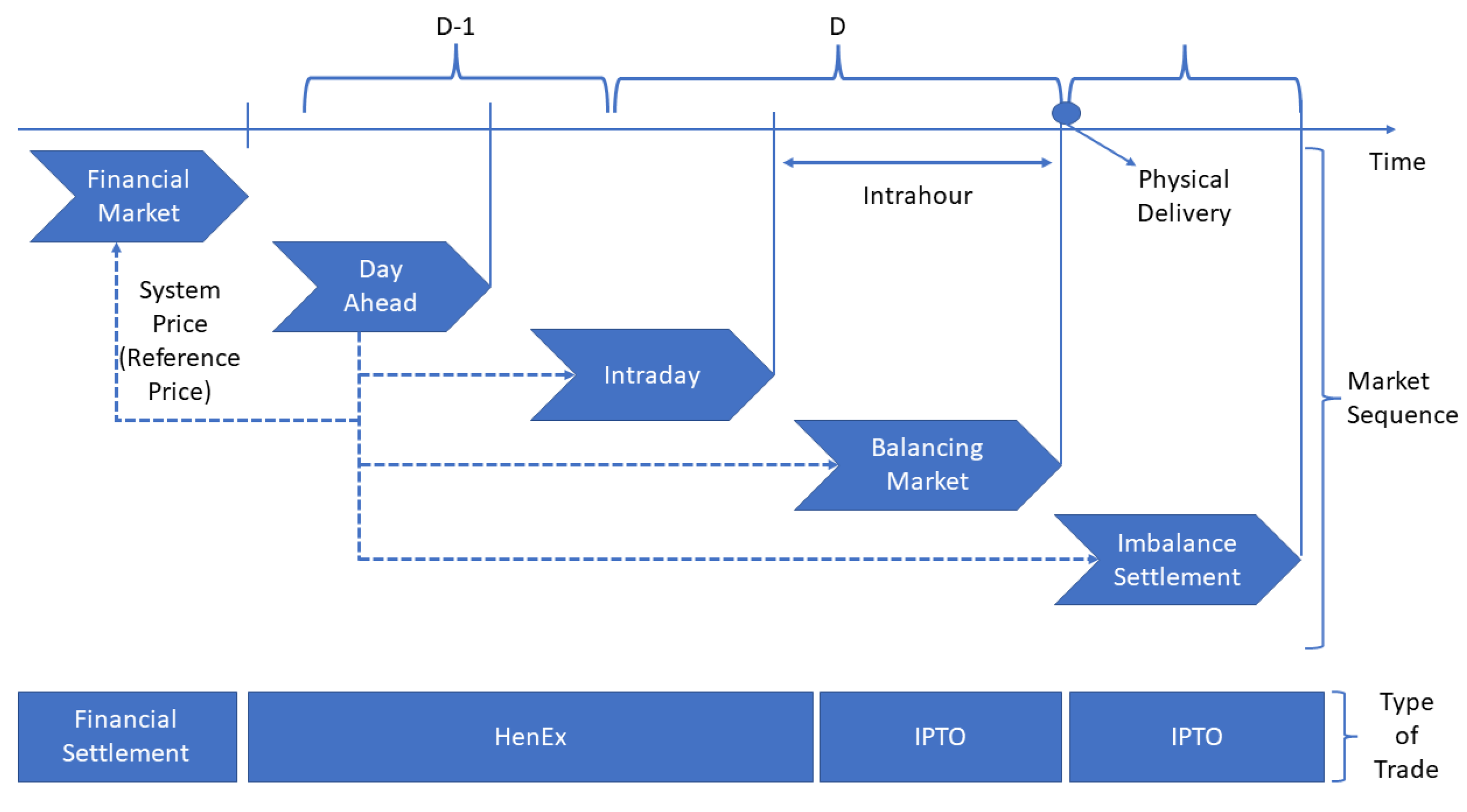
2. The Greek Electricity Market

In Figure 1, an overview of the electricity markets in Greece is presented. Implementation of the Target Model in Greece was launched on 1 November 2020, consistent with EU policy rules (Third Energy Package, Directive 2009/72/EC [15]). The framework for the Target Model includes the forward market (FM), the day-ahead market (DAM), the intra-day market (IDM) and the balancing market (BM).

The Hellenic Energy Exchange (HEnEx) is responsible for the operation of the FM, DAM and IDM, while the BM is operated by the Greek TSO (called the Independent Power Transmission Operator or IPTO). The forward market settlements deal with settling future contracts which determine the quantity and price of energy; FM transactions can be executed either over the counter or through the organized energy exchange and can be settled in a cash settlement or via physical delivery. The FM is an important market for hedging market risks and ensuring successful participation in sequential energy markets; market participants can mitigate their exposure to price volatility in the spot markets. In the DAM, transactions with physical delivery on a specific day D are settled. Participants (both from the supply and demand sides) submit their purchase/sale offers on the previous calendar day (D-1) for physical delivery at each market time unit. Finally, the latest market in the time sequence operated by HEnEX is the IDM where participants may change their positions, taking into account the latest market, weather and operational conditions, and submit offers to buy and/or sell on the same day D. The IDM, where energy is traded continuously, is a particularly useful market for RES participants as they can correct their DAM positions by taking into account the latest weather and market conditions to manage their deviations and risk exposure.

Since system imbalance predictions are directly connected to the BM operation, we briefly present a description of the BM. The purpose of the BM is to correct the imbalances between production and demand in real-time, maintain an uninterrupted supply of energy with predicted quality characteristics, while considering the participants’ market schedule commitments in the previous markets. The BM is divided into the balancing power market, the balancing energy market and the discrepancy clearing process. In the Hellenic BM, the model of the central distribution (central dispatch) of the units is adopted by the TSO through the execution of a security-constrained unit commitment-based integrated scheduling process (ISP), which co-optimizes energy and ancillary service offers in 30 min intervals. Ancillary services are settled based on the ISP process results, while the balancing energy is settled in the subsequent real-time balancing market, which is executed every 15 min by deploying the commitment schedule of units from the ISP. BM participants are characterized as representatives of the balancing responsible parties and/or the balancing service providers. The balancing service providers, as part of their participation in the BM, may submit the following offers: (a) upward and downward frequency conservation reserve (FCR) offers; (b) upward and downward automatic frequency restoration reserve (aFRR) offers; (c) upward and downward manual frequency restoration reserve (mFRR) offers; and (d) upward and downward balancing energy offers.

3. The Proposed Forecasting Methodology

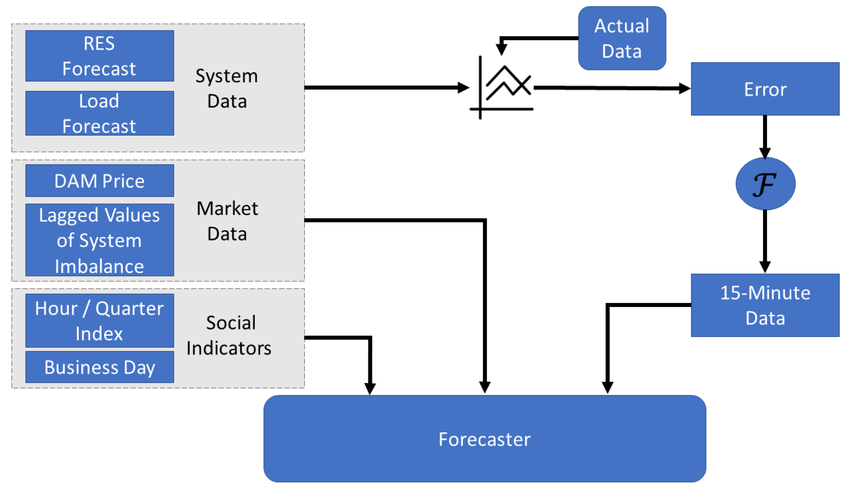
3.1. Architecture of the Forecasting Solution

In Figure 2, the detailed architecture of the proposed solution is illustrated. For the analysis, a set of external predictors are included, which are used to predict the output of the response variable. In our study, the predictors are divided into the following groups:

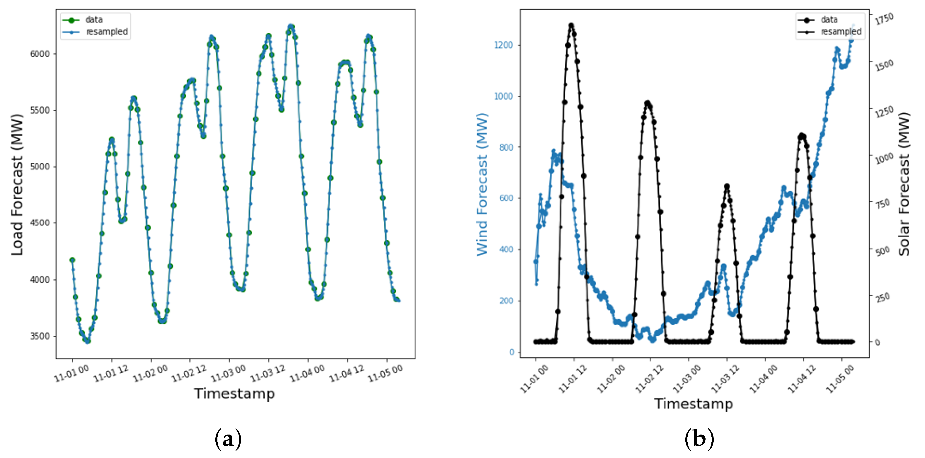
• System data (system demand, RES forecast, RES actual production).
• Market data (DAM price, lagged DAM price, lagged values of system imbalance).
• Social indicators (hour index, quarter index, business day, etc.).

These predictors are selected due to their high predictive power in system imbalance forecasting. They not only capture the key drivers, which affect the supply and demand dynamics within the system, but also reflect information on the market side. Firstly, the module receives the forecasted system data values both for the generation and demand resources. The forecasted data is then compared with the actual values, and the respective forecast error is calculated. Then, a fast Fourier transformation (FFT) is applied to modify the sampling rate of the errors, leading to time-series data of 15 min resolution; this resolution has the desired granularity for the determination of system imbalance volumes.

The set of external predictors is not limited to the system data. Market data are also included and have been proven to be of great importance. To be more specific, the DAM price can provide useful insights since it is directly related to the market and system conditions (e.g., energy mix, RES penetration, peak load, etc.). Additionally, since there is a significant correlation of the real-time system imbalance with the past system imbalance values, the most critical system imbalance lags are also included.

Finally, in the model, some social indicator indices are also included to incorporate information related to seasonalities, which can greatly affect the accuracy of the algorithms.

3.2. Fourier Transform Resampling

As already mentioned in the methodology section, the granularity of the balancing market data differs from the granularity of the system data (system demand and RES). Therefore, a resampling technique is applied to the system data to align the granularity of both sets of data (i.e., increase the sampling rate of the system data) in order to be used in the forecasting model.

In this study, the fast Fourier transform is used for the resampling process. The three key steps of the FFT analysis which are implemented are explained below:

• Transform the original signal to the frequency domain using the FFT:
  $$X\left(k\right)={\sum }_{n=0}^{N-1}x\left(n\right)e^{-j2\pi kn/N},$$

  where N is the number of samples in $x\left(n\right)$.
• Modify the frequency components to achieve the desired sampling rate. In this case, hourly frequency data are transformed to 15 min data by zero-padding the frequency components:
  $$X^{\prime }\left(k\right)=\left[\begin{array}{c}X\left(k\right)00\dots 0\end{array}\right],$$

  where the number of zeros is equal to the desired increase in the number of samples.
• Transform the modified frequency components back to the time domain using the inverse FFT:
  $$x^{\prime }\left(n\right)=\frac{1}{N}{\sum }_{k=0}^{N-1}{X}^{\prime }\left(k\right)e^{j2\pi kn/N}$$

  .

In Figure 3, the FFT results for an indicative period are illustrated, in which the original 1 h resolution time series is transformed into 15 min resolution data.

3.3. Models and Metrics for System Imbalance Forecasting

In this study, three (3) different algorithms were tested for system imbalance forecasting: multivariate linear regression (LR), random forest (RF) and long short-term memory (LSTM). All the algorithms produce deterministic values of system imbalance and were tested both for 15-minute- and 1-hour-ahead forecasting horizons. The specific algorithms have been extensively studied in the literature, and were, therefore, also selected to be examined for the Greek balancing market. In all, the algorithm selection covers a wide range of predictive models, ranging from relatively simple linear models to more sophisticated and complex non-linear models. In multivariate linear regression, a linear statistical relationship between the dependent variable (system imbalance) and the set of independent variables (market data, system data, social indicators) is assumed. The other two algorithms considered in the study can both capture non-linear relationships between the predictors, but differ significantly in terms of producing the forecast. Specifically, in RF a large number of decision trees is combined to make the prediction, each trained on a random subset of the data and using a random subset of the available features. This significantly reduces the risk of overfitting, which happens quite often in ML algorithms. RF is a particularly useful prediction algorithm when dealing with datasets with complex interactions between the variables. Lastly, LSTM is a particular type of recurrent neural network (RNN), which is suited for processing sequences of data (e.g., time series). The memory cells allow an LSTM network to capture long-term dependencies in sequential data and, thus, reveal dependencies which are not captured by the standard models.

The employed metrics in this study for evaluating the performance of the forecasting algorithms were the R-squared ($R^2$), the root mean square error ($RMSE$), and the mean absolute error ($MAE$). The $R^2$ measures the proportion of the dependent variable’s variance which is explained by the independent variables in a regression model. The $RMSE$ measures the standard deviation of the residuals (prediction errors), while the $MAE$ measures the average of the absolute differences between the actual values and the forecasted values. The units for both the RMSE and MAE are the same as the unit of the data in the target variable, while the $R^2$ may not have a unit of measurement, but ranges from 0 to 1. Higher $R^2$ values indicate a better fit of the model to the data. The mathematical formulations of the metrics are given below:

$$R^2=1-\frac{{\sum }_{i=1}^n{(y_i-\widehat{y_i})}^2}{{\sum }_{i=1}^n{(y_i-\overline{y})}^2}$$

(1)

$$RMSE=\sqrt{\frac{1}{n}\sum _{i=1}^n{(y_i-{\widehat{y}}_i)}^2}$$

(2)

$$MAE=\frac{1}{n}\sum _{i=1}^n|y_i-\widehat{y_i}|$$

(3)

where ${\mathrm{y}}_i$ denotes the true value, $\widehat{y_i}$ shows the predicted value, and n indicates the number of fitted points.

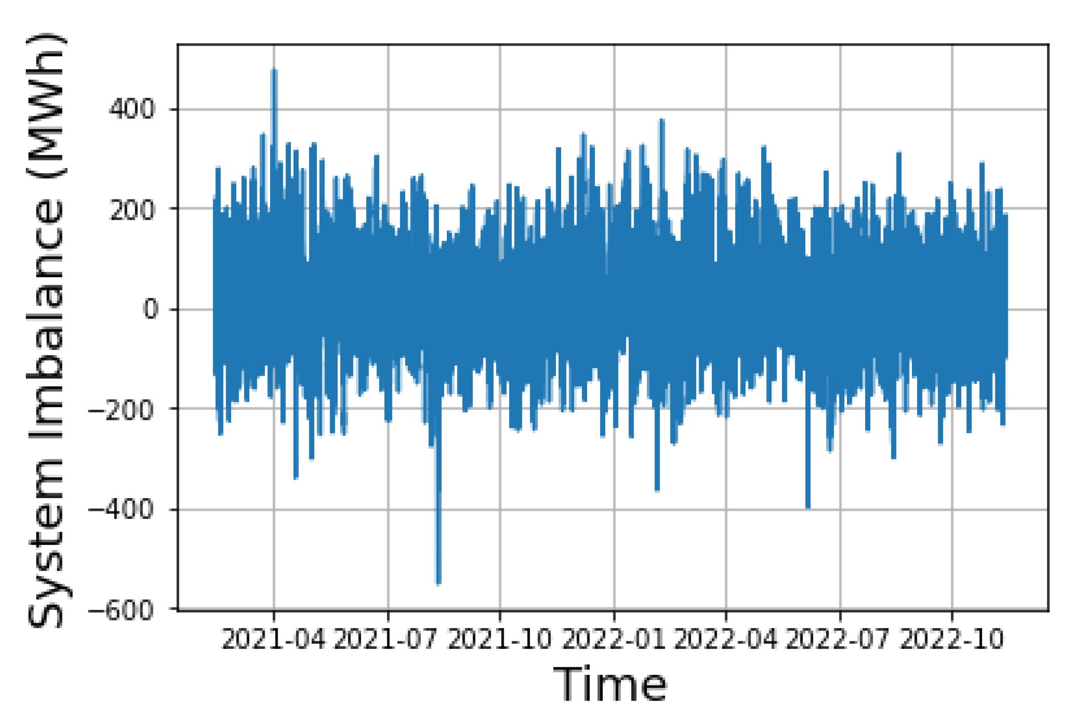
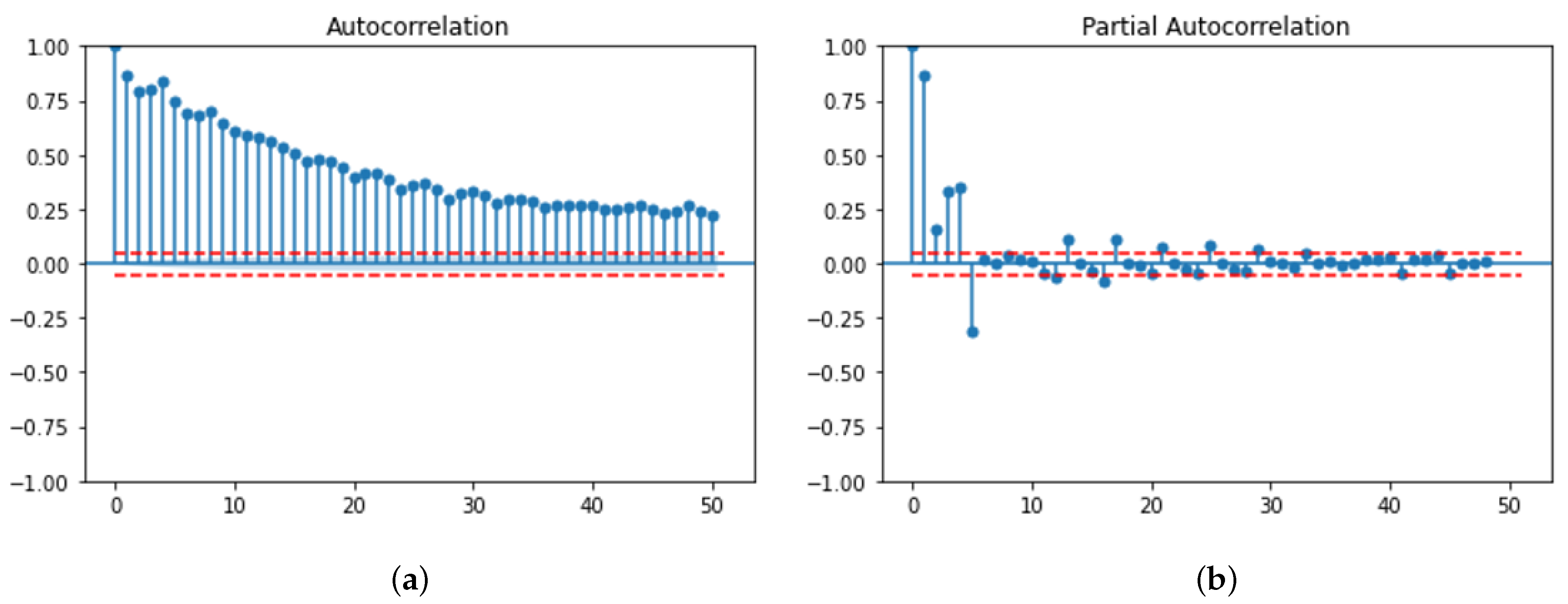
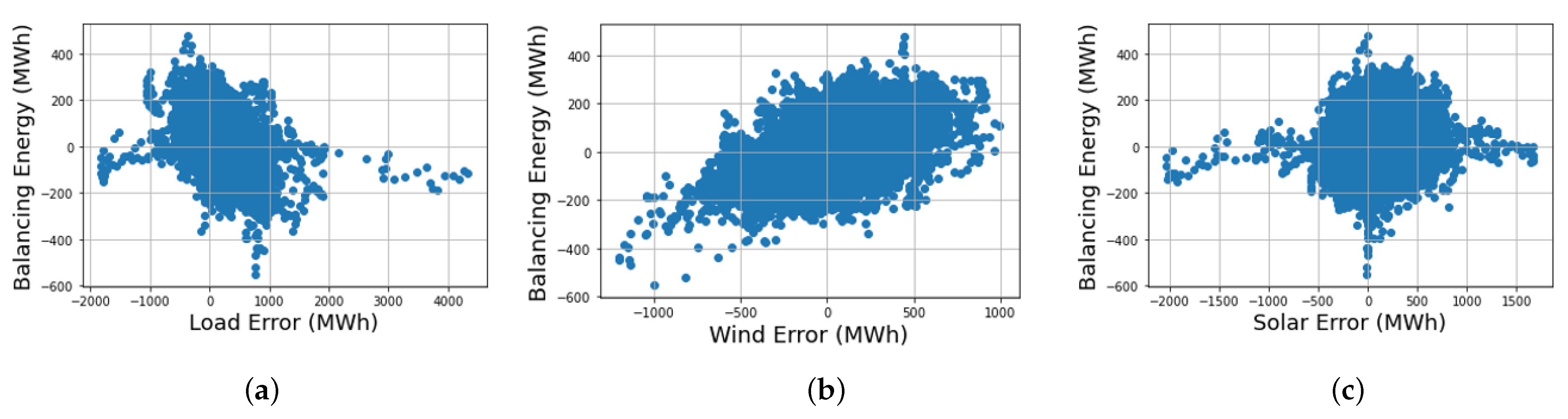
4. Statistical Analysis of the Greek Case Study

The balancing market data considered in this study covered the first period of operation of the balancing market platform in Greece. The market data were downloaded from the IPTO’s web portal [16], while the system data were extracted from ENTSOE’s transparency platform [17]. The examined period was from 13 February 2021 until 13 November 2022. The data from November 2020 (starting date of the BM platform) until the starting date of our analysis data were disregarded since this was considered a trial period for all the participants, potentially leading to erroneous conclusions in our analysis. In

Table 1. Key statistics on the Greek system imbalance (MWh).

	2021	2022
Average	11.42	6.64
Standard Deviation	80.99	76.28
25th Quantile	−39.20	−41.31
50th Quantile	10.10	3.61
75th Quantile	59.86	51.51

, some statistical insights on the system imbalance in 2021 and 2022 are given, while in Figure 4, the respective plot for the whole period is illustrated.

In Figure 5, the autocorrelation and partial autocorrelation plot of the Greek system imbalances are presented. The red dashed line depicts the 95% confidence interval. The autocorrelation shows the correlation of the system imbalance variable at time t with the corresponding values at time t-k, while the partial autocorrelation measures the correlation between the system imbalance variable and the indicated lag without accounting for the effect of the intermediate lags. In our case, the system’s imbalance volume is highly correlated with the first five lags, as illustrated by the partial autocorrelation plot. To this end, the first five lags should be added as external variables and will have a high predictive influence on the results (when applicable). Artificially generated data, which are deducted from these lags, are also suggested to be included (e.g., the average value of the first five lags). Finally, in Figure 6, the correlations of the system imbalance with the system load error, wind production error and solar production error are depicted. The error is defined as the difference between the forecasted values and the actual values, as defined in the Methodology section in Figure 2. It is clear that the correlation was the highest in the case of the wind production error (${\rho }_{xy}=0.5$), indicating that the system imbalance moves in the same direction as the error, but with lower magnitude. The respective Pearson coefficients for the load and solar error were lower, for ${\rho }_{xy}=-0.34$ and ${\rho }_{xy}=0.21$, respectively. Finally, the 95% confidence interval for the correlation coefficients were calculated: [0.49, 0.51] for the wind production error, [−0.35, −0.33] for the load error, and [0.2, 0.22] for the solar production error [18]. The extensive size of the examined dataset, consisting of approximately 65.000 recordings, guarantees the robustness of the calculated correlation coefficients.

5. Forecasting Results

For the evaluation of the different forecasting algorithms and the hyperparameter tuning of the model parameters, a time-series cross-validation methodology was employed. For cross-validation, the original dataset was split into training, validation and test sets, enabling evaluation of the model performance in a more robust way.

Two forecasting horizons were considered in the analysis: 15-minute- and 1-hour-ahead forecasts. In

Table 2. Evaluation metrics of the forecasting algorithms.

		$R^2$ (-)	RMSE (MWh)	MAE (MWh)
15 min forecast	Linear Regression	0.77	33.23	24.41
	Random Forest	0.84	26.93	19.63
	LSTM	0.83	28.12	20.64
1 h forecast	Linear Regression	0.68	39.64	29.75
	Random Forest	0.72	36.53	27.01
	LSTM	0.66	40.04	30.27

, the regression metrics for the three developed models are compared.

The results indicate that the random forest model was the optimal selection for both the forecasting horizons. Specifically, for a 1 h forecasting horizon, random forest was more accurate by 7% compared to linear regression and by 9% compared to LSTM. In the case of the 15 min forecasting horizon, the improvement was even higher, leading to a 4.2% accuracy increase compared to LSTM and an almost 18% increase compared to linear regression.

There are several reasons for the the predictive accuracy of the random forest algorithm in system imbalance forecasting. The non-linearities which exist between the system data (demand and RES production) and the target variable can be more accurately captured in the ensembling method that the random forest methodology relies on. Additionally, there is greater resilience to outliers, which can have a large effect on the parameter estimates, and are prevalent in the first months of the training data. In terms of data requirements, the random forest methodology can perform significantly better compared to neural network approaches (e.g., LSTM), which usually require a larger amount of training data. The analysis data covers a small period of time since the balancing market in Greece is a relatively new market, thus limiting the accuracy of the LSTM methodology. Finally, the training time of the algorithms should also be accounted for as an important parameter since the application requires real-time operating actions by the TSO for the activation of balancing reserves. The training time of the random forest methodology was about 18 s, while the corresponding time for the LSTM methodology accounts was 156 s.

In Figure 7, a plot showcasing the results for the last day of the test set is presented. The specific day is presented as the volume of the system imbalance is within the indicative range for the whole period. The trend is captured by all the forecasting algorithms; the random forest methodology appears to have the smallest deviations in the extreme values, which are also reflected in the presented metric results. In any case, the results of this study can provide useful insights into the system imbalance forecasting problem and offer credence to the argument that it can be used as a complementary tool in the TSO’s operational processes.

6. Conclusions

In the paper, a forecasting tool for the prediction of system imbalance in the Greek power system has been presented, developed and analyzed in detail. The forecasting tool is comprised of a list of external system and market predictors. Three different algorithms have been compared for two different forecasting horizons. In both cases, the random forest algorithm proved to be the most accurate and computationally more efficient compared to the linear regression and standard neural network methodologies. Especially for the short time horizon of the study (15 min), the improvement achieved by the random forest model was considerably higher compared to the 1 h forecasting horizon.

Nevertheless, it is clear that system imbalance prediction is comprised of many different parts and prediction requires information from various sources. The error coming from the system data cannot fully explain the imbalances, and additional explanatory variables should be included to improve the accuracy of the algorithm (e.g., strategic bidding, operational, commercial and transmission constraints, outages modelling, etc.). The resulting data provide strong credence to the claim that the proposed methodology can significantly improve the system imbalance prediction process of a TSO and contribute efficiently to least-cost energy procurement and more economical dispatch of the balancing reserves.

References

1. Zimmermann, F.; Keles, D. State or market: Investments in new nuclear power plants in France and their domestic and cross-border effects. Energy Policy 2023, 173, 113403. [Google Scholar] [CrossRef]
2. IPTO. Preliminary Draft of the Ten Year Development Plan of HETS for the Period 2024–2033. Available online: https://www.admie.gr/en/nea/anakoinosi/preliminary-draft-ten-year-development-plan-hets-period-2024-2033 (accessed on 1 February 2023).
3. Papalexopoulos, A.D.; Hesterberg, T.C. A regression-based approach to short-term system load forecasting. IEEE Trans. Power Syst. 1990, 5, 1535–1547. [Google Scholar] [CrossRef]
4. Shahid, F.; Zameer, A.; Muneeb, M. A novel genetic LSTM model for wind power forecast. Energy 2021, 223, 120069. [Google Scholar] [CrossRef]
5. Gao, F.; Guan, X.; Cao, X.R.; Papalexopoulos, A. Forecasting power market clearing price and quantity using a neural network method. In Proceedings of the Power Engineering Society Summer Meeting, Seattle, WA, USA, 16–20 July 2000; Volume 4, pp. 2183–2188. [Google Scholar]
6. Lago, J.; Marcjasz, G.; De Schutter, B.; Weron, R. Forecasting day-ahead electricity prices: A review of state-of-the-art algorithms, best practices and an open-access benchmark. Appl. Energy 2021, 293, 116983. [Google Scholar] [CrossRef]
7. Elia Group. Documentation of the Methodology Used for the System Imbalance Forecast Publications. Available online: https://www.elia.be/en/grid-data/balancing/system-imbalance-forecasts (accessed on 1 February 2023).
8. Garcia, M.P.; Kirschen, D.S. Forecasting system imbalance volumes in competitive electricity markets. IEEE Trans. Power Syst. 2006, 21, 240–248. [Google Scholar] [CrossRef]
9. Kratochvíl, Š. System Imbalance Forecast. Ph.D. Thesis, Czech Technical University, Prague, Czech Republic, 2016. Available online: https://dspace.cvut.cz/bitstream/handle/10467/67662/Disertace_ŠtěpanKratochvil2016.pdf?sequence=1 (accessed on 1 February 2023).
10. Contreras, C. System Imbalance Forecasting and Short-Term Bidding Strategy to Minimize Imbalance Costs of Transacting in the Spanish Electricity Market. 2016. Available online: https://repositorio.comillas.edu/xmlui/handle/11531/16621 (accessed on 1 February 2023).
11. Salem, T.S.; Kathuria, K.; Ramampiaro, H.; Langseth, H. Forecasting intra-hour imbalances in electric power systems. In Proceedings of the AAAI Conference on Artificial Intelligence, Honolulu, HI, USA, 27–31 January 2019; Volume 33, pp. 9595–9600. [Google Scholar]
12. Ioannidis, F.; Kosmidou, K.; Andriosopoulos, K.; Everkiadi, A. Assessment of the Target Model Implementation in the Wholesale Electricity Market of Greece. Energies 2021, 14, 6397. [Google Scholar] [CrossRef]
13. Makrygiorgou, J.J.; Karavas, C.-S.; Dikaiakos, C.; Moraitis, I.P. The electricity market in Greece: Current status, identified challenges and arranged reforms. Sustainability 2023, 15, 3767. [Google Scholar] [CrossRef]
14. Papavasiliou, A. An Overview of Probabilistic Dimensioning of Frequency Restoration Reserves with a Focus on the Greek Electricity Market. Energies 2021, 14, 5719. [Google Scholar] [CrossRef]
15. Third Energy Package. Available online: https://energy.ec.europa.eu/topics/markets-and-consumers/market-legislation/third-energy-package_en (accessed on 1 February 2023).
16. IPTO Balancing Market Data. Available online: https://www.admie.gr/en/market/market-statistics/detail-data (accessed on 1 February 2023).
17. ENTSO-E Transparency Platform. Available online: https://transparency.entsoe.eu/dashboard/show (accessed on 1 February 2023).
18. Tian, L.; Wilding, G.E. Confidence interval estimation of a common correlation coefficient. Comput. Stat. Data Anal. 2008, 52, 4872–4877. [Google Scholar] [CrossRef]
Figure 1. Overview of electricity markets.
Engproc 39 00018 g001
Figure 2. Architecture of the proposed forecasting solution for system imbalance prediction.
Engproc 39 00018 g002
Figure 3. FFT resampling. (a) System load (b) RES (wind and solar).
Engproc 39 00018 g003
Figure 4. System imbalance in the Greek power system for the period February 2021–November 2022.
Engproc 39 00018 g004
Figure 5. (a) Autocorrelation and (b) partial autocorrelation for the first 50 lags of system imbalance (the red dashed line indicates the 95% confidence interval).
Engproc 39 00018 g005
Figure 6. Correlation between system imbalance and (a) system load error, (b) wind production error, (c) solar production error.
Engproc 39 00018 g006
Figure 7. Forecasting results for system imbalance (13 November 2022).
Engproc 39 00018 g007