Proceeding Paper

A Deep Learning Model Based on Multi-Head Attention for Long-Term Forecasting of Solar Activity †

by
Adriana Marcucci
1,‡,
Giovanna Jerse
2,*,‡,
Valentina Alberti
2 and
Mauro Messerotti
2
1
Department of Physics, University of Trieste, Via A. Valerio 2, 34127 Trieste, Italy
2
Astronomical Observatory of Trieste, INAF, Via G. Tiepolo 11, 34143 Trieste, Italy
*
Author to whom correspondence should be addressed.
Presented at the 9th International Conference on Time Series and Forecasting, Gran Canaria, Spain, 12–14 July 2023.
These authors contributed equally to this work.
Eng. Proc. 2023, 39(1), 16; https://doi.org/10.3390/engproc2023039016
Published: 29 June 2023
(This article belongs to the Proceedings of The 9th International Conference on Time Series and Forecasting)

Abstract

:
The accurate long-term forecasting of solar activity is crucial in the current era of space explorations and in the study of planetary climate evolution. With timescales of about 11 years, these forecasts deal with the prediction of the very general features of a solar cycle such as its amplitude, peak time and period. Solar radio indices, continuously measured by a network of ground-based solar radio telescopes, are among the most commonly used descriptors to characterise the solar activity level. They can act as proxies for the strength of ionising radiations, such as solar ultraviolet and X-ray emissions, which directly affect the atmospheric density. In a preliminary comparative study of a selection of univariate deep-learning methods targeting medium-term forecasts of the F10.7 index, we noticed that the performance of all the considered models tends to degrade with increasing timescales and that this effect is smoother when a multi-attention module is included in the used neural network architecture. In this work, we present a multivariate approach based on the combination of fast iterative filtering (FIF) algorithm, long-short term memory (LSTM) network and multi-attention module, trained for the present solar cycle forecasting. Several solar radio flux time series, namely F3.2, F8, F10.7, F15, F30, are fed into the neural network to forecast the F10.7 index. The results are compared with the official solar cycle forecasting released by the Solar Cycle Prediction Panel representing NOAA, NASA and the International Space Environmental Services (ISES) to highlight possible discrepancies.

1. Introduction

The Sun is a moderately active G2V-type star, whose current age is 4.6 billion years. Its magnetic activity follows a quasi-periodic variation of about 11 years, after which the magnetic field completely flips. Over this time period, the number of sunspots that appear on the photosphere increases and decreases in a cyclic way, generating the so-called solar cycle, which is responsible for driving the short-to-long-term fluctuations in solar activity. Short-term solar variability includes transient events such as radiation outbursts, highly energetic particles and plasmoids, which characterise space weather (SWx) and can influence currently operating space-reliant technologies, planetary atmospheres and magnetospheres within a few days. The dynamo mechanism that works in the solar interior drives the long-term fluctuations in solar output that determine the space climate, which can impact planetary climate over decadal or longer timescales [1].
In this work, we focus on the prediction of the activity level over a period of 11 years corresponding to one solar cycle. The result can be used as input to various atmospheric models that characterise the physical state of the Earth’s upper atmosphere, such as the thermosphere and ionosphere, and are used for satellite orbit determination, re-entry services, collision avoidance manoeuvres and modelling of the evolution of space debris [2]. Variations in the thermospheric density, in fact, cause variations in the atmospheric drag affecting orbiting satellites, which need to be carefully taken into account when planning spacecraft operations. Moreover, the abundance in the heliosphere of highly energetic particles, known as galactic cosmic rays, shows a periodicity that anticorrelates with solar activity. Cosmic rays constitute a hazard to space instruments and human missions. Hence, an increase in the precision at which we can predict their occurrence is critical.
Historically, long-term forecasts of solar activity have been based on the solar sunspot number (SSN), the weighted sum of the numbers of sunspots and sunspot groups on the solar disk at one time, present in records since 1600. They are good descriptors of almost all other features on the Sun, including active regions, plages, flares, prominences, and, to some extent, changes in the evolution of coronal and solar wind features [3]. Recent studies have started to consider solar radio emission at 10.7 centimetres as an alternative index to describe the solar variability. The F10.7 index is the integrated emission from the whole solar disk at the radio wavelength of 10.7 cm (2800 MHz). It results from thermal ionisation at the boundary between the photosphere and the chromosphere and from magnetic resonance above sunspots and plages [4]. In general, it is used as a proxy for the full-disk flux at the ultraviolet (UV), extreme ultraviolet (EUV), X-ray, Ca II and Mg II wavelengths, and for the total solar irradiance. Records of its values have been consistently measured by ground-based radio telescopes in Canada since 1947, on a day-by-day basis, in any weather condition. Penticton Radio Observatory in British Columbia provides a number of other radio indexes with the same cadence and duration as the F10.7, namely F3.2, F8, F15 and F30, recorded since 1957. They represent the solar flux emissions at different wavelengths measured in solar flux units, where 1 sfu = 10 22   W m 2 H z 1 . Radio waves at different frequencies are emitted at different heights in the solar chromosphere and low corona by plasma layers that have decreasing electron density with increasing altitude: short-wavelength emissions originated at lower altitudes, whereas long-wavelength ones originated at higher altitudes. Hence, we considered exploiting the “tomography” of the solar plasma layers to enhance the performances in solar activity forecasts with a multivariate approach. The majority of models adopted in the space weather framework so far to forecast the short-term trend of empirical time series such as the F10.7 index are statistical models and only a minority of the studies rely on machine learning and deep learning approaches. This number is even smaller if we consider the investigations performed to predict the solar cycle amplitude based on deep learning neural networks [5,6,7,8,9]. In this case, the focus is mainly on the application of classical methods such as support vector regression or single-layer feed-forward neural networks. Since the F10.7 time series is non-linear and non-stationary, we propose a viable approach to cope with its complexity, which decomposes the signal into simpler components and then predicts each of them separately. Decomposition methods, coupled with LSTM neural network, offer a significant enhancement in the field of time series prediction, allowing for a reduction in the chaotic characteristics of the original data. We use the fast iterative filtering (FIF) algorithm [10], which is a robust and stable decomposition signal technique that is suitable for analysing non-linear and non-stationary data, to identify each oscillation component, and discard the short-term ones. The LSTM network is then trained on the decomposed functions that are more correlated with the F10.7 timeseries to predict the solar cycle F10.7 values. In this work, we also adopt the attention-based architecture, which represents one of the main frontiers in deep learning and, to the best of our knowledge, has never been applied for time series forecasting in the space weather context. The attention module is an evolution of the encoder–decoder model, which has been developed to improve performance when using long input sequences.
The remainder of the paper is organized as follows. Our proposed multi-variate model for the solar cycle F10.7 prediction is illustrated in Section 2. Section 3 presents our 25th solar cycle predictions and discussion. Our results will be compared with the official forecasts given by the NOAA Space Weather Prediction Center to verify if they can be considered a good alternative to reproducing long-term variations in solar activity. Finally the conclusion of the paper is given in Section 4.

2. Deep Learning LSTM-Based Method for Long-Term F10.7 Time Series Forecasting

In this work we propose a long short-term emory (LSTM) neural network based on the Mmulti-attention architecture for multivariate time series data predictions of the 25th solar cycle. Our deep learning LSTM-based model has four processes, as shown in Figure 1.
The data preparation and processing will be discussed in detail in Section 2.1. This part is fundamental to preparing the dataset that will be used as input to the LSTM-based neural networks. The prediction module is responsible for analyzing and predicting data based on the input data set and the attention value processed by the attention mechanism, which calculates the distribution of weights of each sequence. The output is the long-term F10.7 forecasting. The basics of the LSTM and multi-attention network that were used to develop the proposed model are revised, respectively in the Section 2.2 and Section 2.3, while the model architecture will be described in Section 2.4.

2.1. Data Description and Preparation

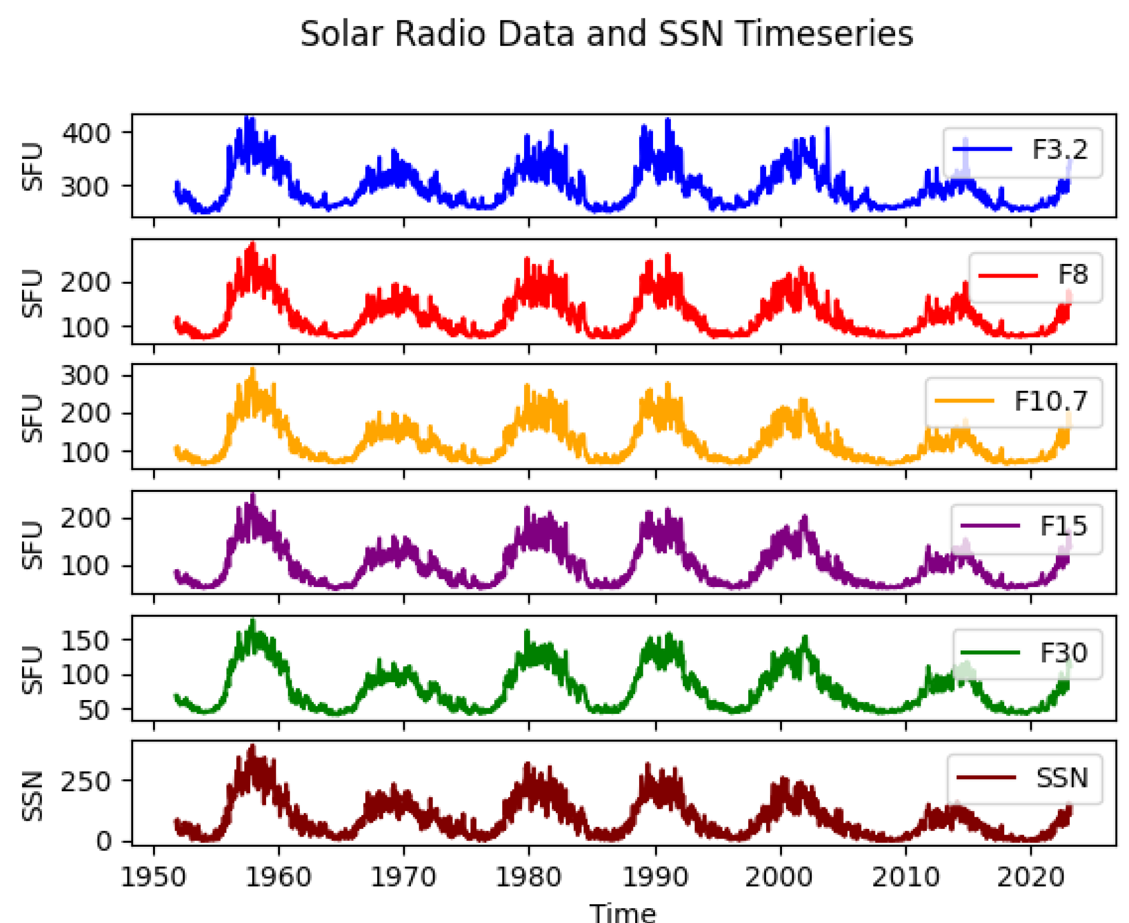
The multivariate data set used in our paper incorporates six features: five solar radio fluxes and the International Sunspot Number from 2 November 1951 to 14 March 2023 (see Figure 2).
These data were obtained thanks to the LASP Interactive Solar IRradiance Datacenter (LISIRD) portal [11]. The service aims to facilitate solar and heliophysics studies by allowing the researcher to easily discover, visualize, and download data from a variety of space missions and ground-based facilities: the extensiveness of the provided/gathered data sets and the completeness of their description (metadata), along with the plotting capabilities and a very intuitive interface, make it a very powerful resource. The service is maintained by the Laboratory for Atmospheric and Space Physics (LASP) of the University of Colorado, Boulder [12].
Solar radio data are obtained from an external service, the Collecte Localisation Satellites (CLS), that focuses on modelling the upper atmosphere to predict low Earth satellite orbits [13]. Five different wavelengths are available and sourced by the radio telescopes situated in Toyokawa, Nobeyama, Ottawa and Penticton (see the list below for details) [13].
  • F30: 30 cm radio flux from Toyokawa (historical data) and Nobeyama (recent data)
  • F15: 15 cm radio flux from Toyokawa (historical data) and Nobeyama (recent data)
  • F10.7: 10.7 cm radio flux from Ottawa (historical data) and Penticton (recent data)
  • F8: 8 cm radio flux from Toyokawa (historical data) and Nobeyama (recent data)
  • F3.2: 3.2 cm radio flux from Toyokawa (historical data) and Nobeyama (recent data)
Given the geographical position of the observatories, data were recorded at different times, namely: 03:00 UT Nobeyama and Toyokawa; 17:00 UT Ottawa (until 31 May 1991); 20:00 UT Penticton (since 1 June 1991). CLS performs the initial processing of the data to fill any potential gaps using an expectation-maximization algorithm and to replace values with the residual error above a certain threshold with one calculated via an auto-regressive model [13]. It also allows for data adjusted at 1AU to be selected, which is more convenient for the satellites’ orbit prediction model. For our study, we relied on the CLs process to prepare the data set, did not attempt to resample the data to a common time grid and considered the adjusted values. The sunspot number time series is derived externally from the sunspot index and long-term solar observations (SILSO) world data Center [14] of the Royal Observatory Belgium in Brussels.
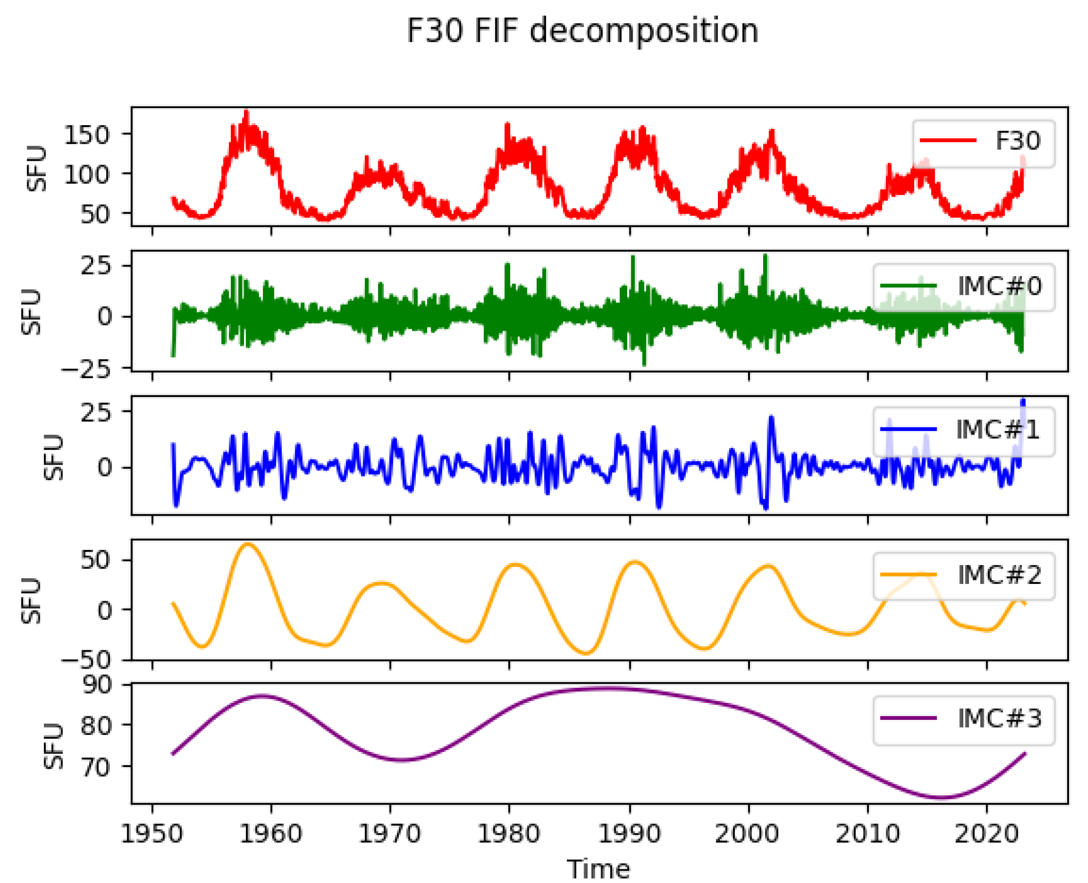
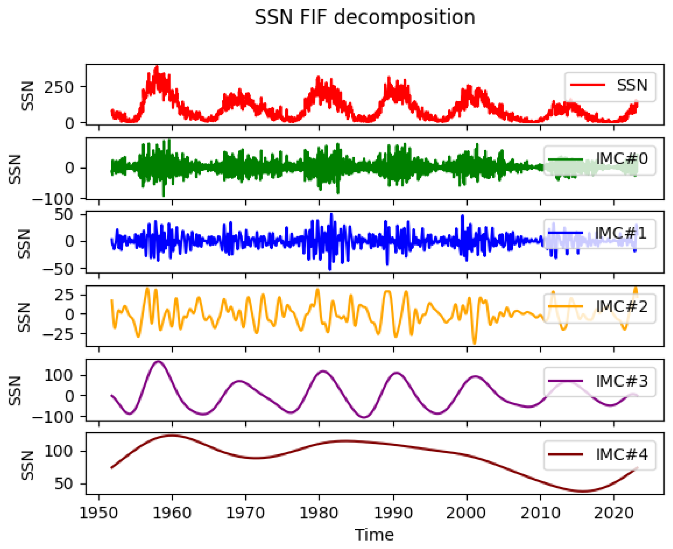
In order to improve the F10.7 long-term prediction capability of our model by reducing the complexity of the original signal, each data set was decomposed using the fast iterative filter (FIF) technique [10]. This decomposition approach decomposes the original signal into components, called intrinsic mode components (IMCs), which are basically oscillatory functions associated with intrinsic variations at various time scales and derived without leaving the time domain. The results of the FIF decomposition of F30 and SSN time-series are given as examples in Figure 3 and Figure 4, respectively.
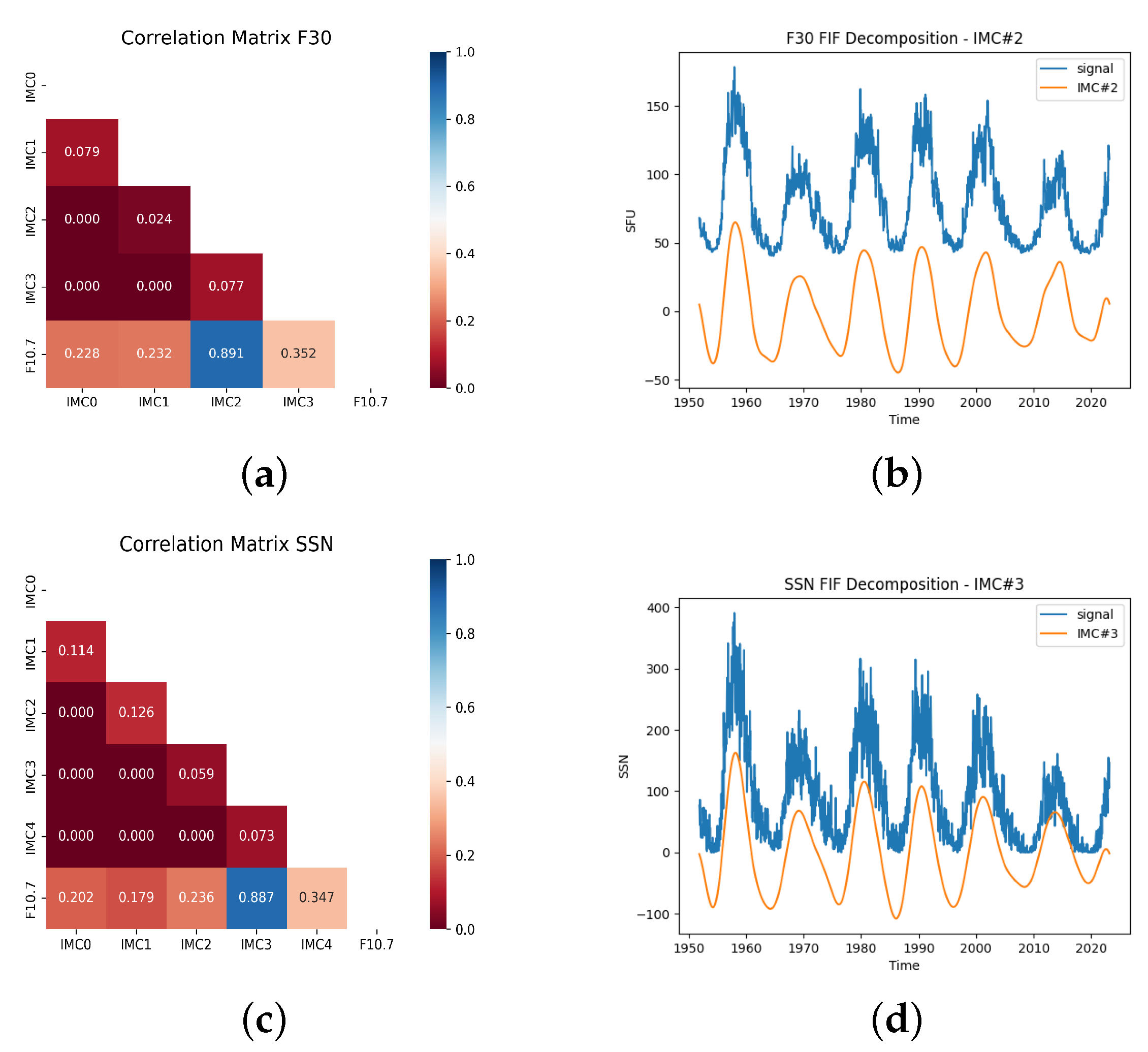
In general lower-order IMCs show a chaotic and random signal behaviour with noise contribution while higher-order IMCs contain lower-frequency components and seem to reproduce oscillations at typical physical time scales, such as the Schwabe cycle (11 years). In order to identify the IMC that follows the Schwabe cycle trend, Pearson’s-based correlation analysis was applied to each IMC of the analysed indexes and the original F10.7 signal. The results of the correlation analysis for F30 and SSN indexes are given in the correlation matrices depicted in Figure 5 (panels a and c, respectively). The IMC of any index with the highest correlation coefficient with the F10.7 time series (plotted in the panels b and d in Figure 5) was treated as a separate time series mediated over a time period of two weeks and given as an input to the multivariate LSTM network to forecast the F10.7 values. The decision to average the data over a bi-weekly interval comes from the need to balance computer performances with accurate long-term predictions.

2.2. LSTM Model

The LSTM networks belong to the family of Recurrent Neural Networks (RNNs) and they have the ability to process entire sequences of data without the memory loss that exists in classic RNN models. They are specifically designed to overcome the long-term dependency problem of the classic RNN models due to the exploding and vanishing gradient. The LSTM model is characterized by a chain-like structure (see Figure 6)—similar to the RNN architecture—of repeating memory modules, known as LSTM cells, with specific features to judge whether the information provided to the network is useful.
In each memory module, a cell state C t at the time t controls the network information using its three gates: the forget, input and output gates. The input gate decides which values in input will use to modify the internal status of the cell. The output gate calculates a vector used to update the memory cell based on the other gates. The forget gate determines a vector used to choose which values of the precedent state should be maintained in the current one.

2.3. Multi-Attention Module

The attention-based architecture was first described and used in [16] and is a technique that mimics human cognitive attention. The attention mechanism is particularly useful to process multiple time series data, since it can reduce the effect of irrelevant information on the results and enhance the influence of related information by assigning different weights and improve prediction results’ accuracy. In this way, it is able to keep track of long-term dependencies in data sequences and reduce the computational effort compared to recurrent or convolutional layers. It can be described as a function that maps a query vector with a set of key-value vector pairs to generate an output. The query vector represents the current state of the model, the keys are used to calculate the similarity scores with the query, and the values vector represents the different features in the input vector. In this work, we specifically used the multi-head-attention (MHA) mechanism, which permits the different heads to focus on different correlations in data and enhance different values in the sequence. Instead of using a single attention function across all the input, it runs the attention algorithm several times in parallel with different learned weights. The independent outputs of each attention module are then concatenated to obtain the final weights. This mechanism can attend to parts of the sequence differently (e.g., longer-term dependencies versus shorter-term dependencies).

2.4. Proposed Multi-Head Attention LSTM Model Architecture

The model architecture used in this work (Figure 7) consists of a three LSTM layers of 12 nodes each, an attention layer with eight heads and, finally, a dense layer, i.e., a layer that is connected deeply, in which each neuron receives input from all neurons of its previous layer. All models were implemented using Python programming language and the Tensorflow library dedicated to multiple machine learning tasks, with Keras as neural network library. In order to validate the forecasting results, we used 80% of the total values as the training set while the remaining 20% served as a validation data set. After training and testing, we used the trained LSTM model to predict F10.7 values and then compared these predicted results with the actual data. In this work, we used the root mean squared error (RMSE), namely the degree of deviation between predicted and observed values, as a performance evaluation metric, defined as follows:
R M S E = 1 N i = 1 N ( y i y i ) 2 ,
where y i and y i are the i t h observed and predicted values, respectively, and N is the number of data points in the testing time series. Figure 8a shows the RMSE of the model at different lead time forecasts. The model performance shows a very stable behaviour in lag size with an RMSE value (see Figure 8a) not exceeding 25%, which proves the overall model prediction effectiveness. As an example, the actual and predicted values of F10.7 index corresponding to a lead time of 80 weeks are plotted in Figure 8b. Our model tends to smooth the prediction curve due to the peculiarity of the attention module to discard less relevant features of the time series and highlight the global trend.

3. Experimental Results and Discussion

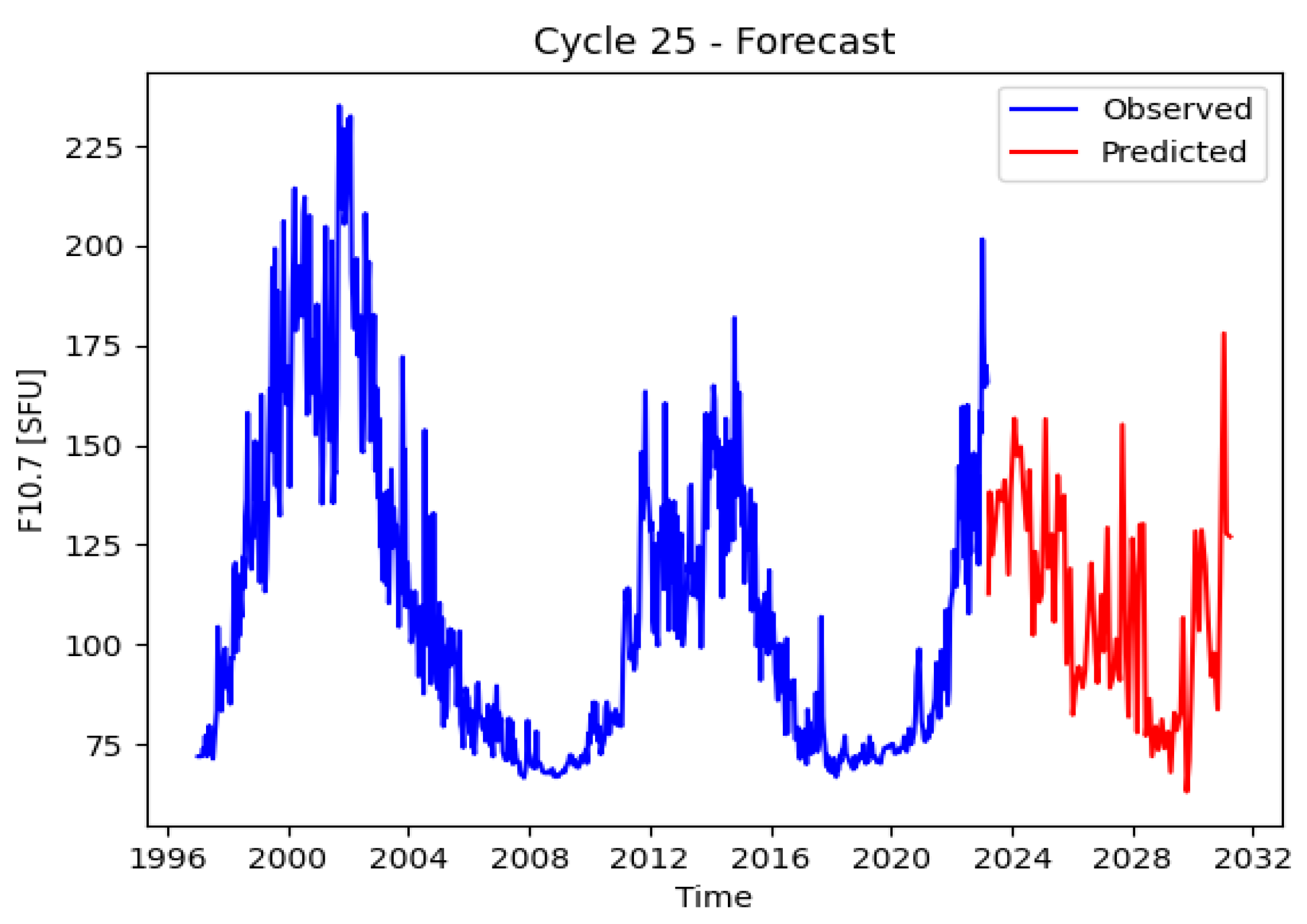
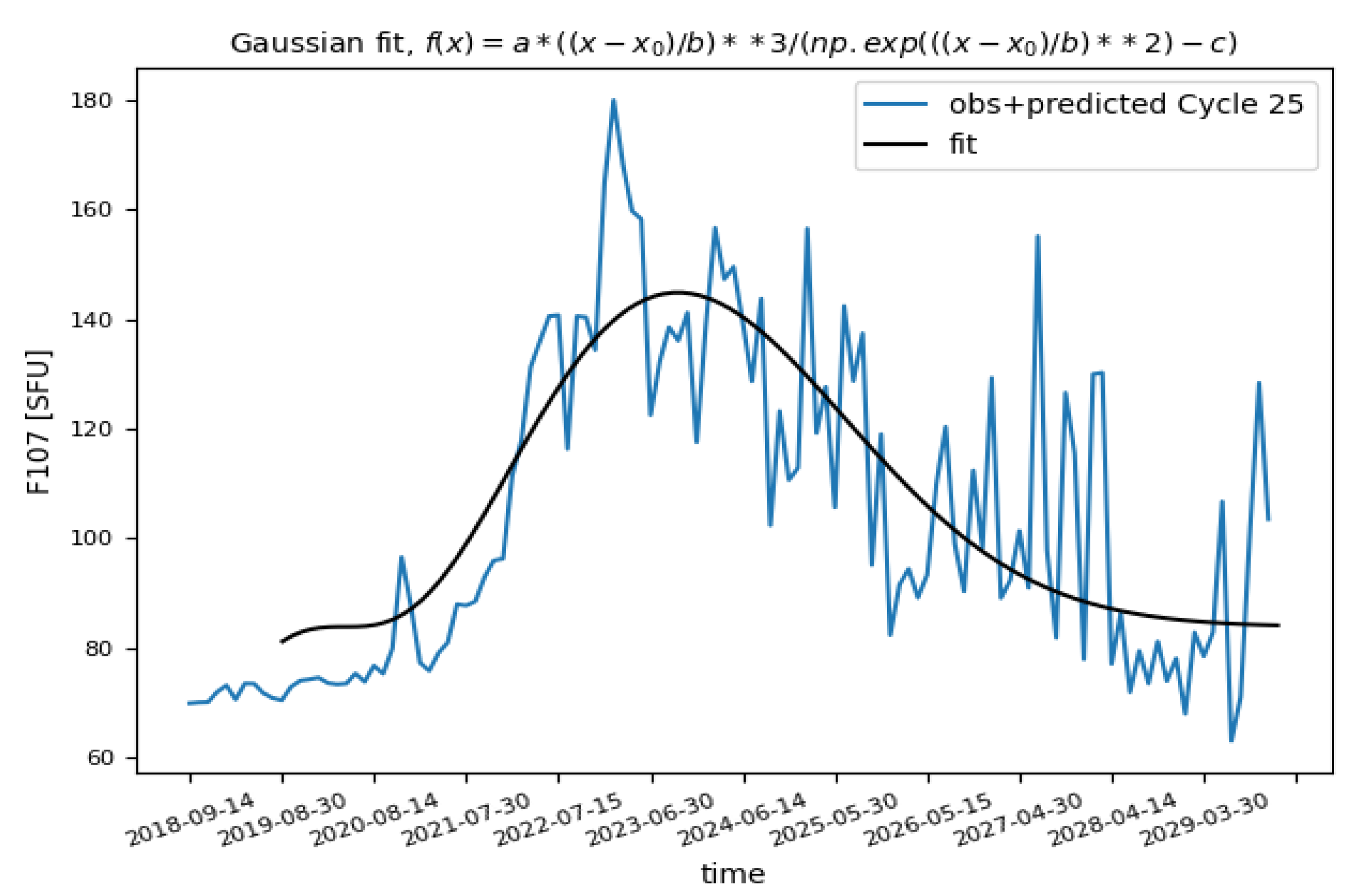
The forecasting result of F10.7 index for the solar cycle 25 are given in Figure 9. In order to characterize the amplitude and peak time of the predicted solar cycle, we fitted the shape of the predicted curve with a function with four free parameters proposed by [17] and [18] of the form
f ( t ) = a ( t t 0 ) 3 / exp [ ( t t 0 ) 2 / b 2 ] c ,
where parameter a represents the amplitude and is directly related to the rate of rise from minimum; b is related to the time in months from minimum to maximum; c gives the asymmetry of the cycle; and t 0 denotes the starting time. This well-known function reproduces both the rise and decay part of the solar cycle and has a more rapid decline after maximum. The curve fitting is given in Figure 10 with the following optimal values: a = 124.33712279 , t 0 = 16.79123391 , b = 32.81850839 , c = 0.6408711 . From the fitted curve, we derived that the predicted F10.7 maximum amplitude for the solar cycle 25 is about 145 ± 25, peaking in November 2023.
We compared our solar cycle 25 forecasting with the official predictions released by the Solar Cycle 25 Prediction Panel and the International Space Environmental Services (ISES) in 2019 April [19]. The Solar Cycle 25 Prediction Panel is an international group of experts co-chaired by the National Aeronautics and Space Administration (NASA), National Oceanic and Atmospheric Administration (NOAA), and International Space Environmental Services (ISES), whose objective is to predict the amplitude of solar cycle 25. These predictions are a synthesis of a variety of prediction methods coming from the scientific community ranging from physical models, precursor methods to statistical inference, machine learning, and other techniques. The Prediction Panel predicted that solar cycle 25 will be similar to solar cycle 24 and will reach a maximum in July 2025 [20] with a peak F10.7 value of 135 ± 10 SFU,(see Figure 11). This prediction is in line with the current general agreement in the scientific literature, which holds that solar cycle 25 will be weaker than average, even if observed values from 2020 to 2022, the first three years of the cycle, are significantly higher than the predicted values. It is evident that our predictions are consistent with the official ones in the peak F10.7 value but our model predicts the 25th solar cycle maximum about 20 months before.

4. Conclusions

In this paper, we present a multivariate deep-learning-based model for solar activity prediction based on a combination of decomposition algorithm, long short-term memory (LSTM) network and multi-attention module. One of the added values of this work consists of the original use of the multi-attention architecture, which has never been used before in this specific field. The study proved the prediction capability of the model using the RMSE evaluation metrics, showing a stable behaviour with increasing forecasting horizon. After the model test analysis presented in this work, we applied our prediction model to Solar cycle 25 forecasting: the peak amplitude of F10.7 is expected to be 145 SFU, while the occurrence of the solar maximum is foreseen by the end of 2023. Our results are in agreement with other studies, such as the forecasting released by the Solar Cycle 25 Prediction Panel, as regards the peak value, but its occurrence is predicted earlier than other forecasts. Future studies could include investigating the impact of other multivariate features such as solar and geomagnetic index on model performance and prediction accuracy.

Author Contributions

All authors have contributed substantially to this work. All authors have read and agreed to the published version of the manuscript.

Funding

This research received no external funding.

Institutional Review Board Statement

Not applicable.

Informed Consent Statement

Not applicable.

Data Availability Statement

The results presented in this document rely on data described in [21]. These data are available from the WDC-SILSO, Royal Observatory of Belgium, Brussels [14]. Data collected by the Solar Radio Monitoring Program with additional processing by the Space Weather Services at Collecte Localisation Satellites (CLS). These data were accessed via the LASP Interactive Solar Irradiance Datacenter (LISIRD) [11].

Acknowledgments

We would like to show our gratitude to Emanuele Papini (Astrophysical Observatory of Arcetri, INAF) for sharing his FIF algorithm in Python [22].

Conflicts of Interest

The authors declare no conflict of interest.

References

  1. Messerotti, M. Space Weather and Space Climate. In Life in the Universe. Cellular Origin and Life in Extreme Habitats and Astrobiology; Seckbach, J., Chela-Flores, J., Owen, T., Raulin, F., Eds.; Springer: Dordrecht, The Netherlands, 2004; Volume 7. [Google Scholar] [CrossRef]
  2. Petrova, E.; Podladchikova, T.; Veronig, A.M.; Lemmens, S.; Virgili, B.B.; Flohrer, T. Medium-term Predictions of F10.7 and F30 cm Solar Radio Flux with the Adaptive Kalman Filter. Astrophys. J. Suppl. Ser. 2021, 254, 9. [Google Scholar] [CrossRef]
  3. Deng, L.H.; Li, B.; Zheng, Y.F.; Cheng, X.M. Relative phase analyses of 10.7cm solar radio flux with sunspot numbers. New Astron. 2013, 23–24, 1–5. [Google Scholar] [CrossRef]
  4. Tobiska, W.K.; Bouwer, S.D.; Bowman, B.R. The development of new solar indices for use in thermospheric density modeling. J. Atmos. Sol.-Terr. Phys. 2008, 70, 803–819. [Google Scholar] [CrossRef]
  5. Prasad, A.; Roy, S.; Sarkar, A.; Chandra Panja, S.; Narayan Patra, S. Prediction of Solar Cycle 25 using deep learning based long short-term memory forecasting technique. Adv. Space Res. 2022, 69, 798. [Google Scholar] [CrossRef]
  6. Warren, H.P.; Emmert, J.T.; Crump, N.A. Linear forecasting of the F10.7 proxy for solar activity. Space Weather. 2017, 15, 1039–1051. [Google Scholar] [CrossRef]
  7. Wang, Z.; Hu, Q.; Zhong, Q.; Wang, Y. Linear multistep F10.7 forecasting based on task correlation and heteroscedasticity. Adv. Earth Space Sci. 2018, 5, 863–874. [Google Scholar] [CrossRef]
  8. Du, Y. Forecasting the daily 10.7 cm solar radio flux using an autoregressive model. Sol. Phys. 2020, 295, 1–23. [Google Scholar] [CrossRef]
  9. Camporeale, E. The challenge of machine learning in space weather: Nowcasting and forecasting. Space Weather. 2019, 17, 1166–1207. [Google Scholar] [CrossRef]
  10. Cicone, A. Iterative Filtering as a direct method for the decomposition of non-stationary signals. arXiv 2018. [Google Scholar] [CrossRef]
  11. Laboratory for Atmospheric and Space Physics. LASP Interactive Solar Irradiance Datacenter; Laboratory for Atmospheric and Space Physics: Boulder, CO, USA, 2005. [Google Scholar] [CrossRef]
  12. LASP Homepage. Available online: https://lasp.colorado.edu/lisird/ (accessed on 16 May 2023).
  13. CLS Homepage. Available online: https://spaceweather.cls.fr (accessed on 16 May 2023).
  14. SILSO Homepage. Available online: https://www.sidc.be/silso/home (accessed on 20 May 2023).
  15. LSTM Networks. Available online: http://colah.github.io/posts/2015-08-Understanding-LSTMs/ (accessed on 10 May 2023).
  16. Bahdanau, D.; Cho, K.; Bengio, Y. Neural Machine Translation by Jointly Learning to Align and Translate. In Proceedings of the 3rd International Conference on Learning Representations, ICLR, San Diego, CA, USA, 7–9 May 2015. [Google Scholar] [CrossRef]
  17. Hathaway, D.H.; Wilson, R.M.; Reichmann, E.J. The Shape of the Sunspot Cycle. Sol. Phys. 1994, 151, 177–190. Available online: https://ui.adsabs.harvard.edu/abs/1994SoPh..151..177H (accessed on 20 May 2023). [CrossRef]
  18. Du, Z.L. The solar cycle: A modified Gaussian function for fitting the shape of the solar cycle and predicting cycle 25. Astrophys. Space Sci. 2022, 367, 20. [Google Scholar] [CrossRef]
  19. Biesecker, D.A.; Upton, L. Solar Cycle 25 Consensus Prediction Update. AGU Fall Meet. Abstr. 2019, 2019, SH13B-03. [Google Scholar]
  20. Solar Cycle Progression. Available online: https://www.swpc.noaa.gov/products/solar-cycle-progression (accessed on 20 May 2023).
  21. Veronig, A.M.; Jain, S.; Podladchikova, T.; Pötzi, W.; Clette, F. Hemispheric sunspot numbers 1874–2020. Astron. Astrophys. 2021, 652, A56. [Google Scholar] [CrossRef]
  22. Papini, E. GitHub Repository. 2022. Available online: https://github.com/EmanuelePapini/FIF (accessed on 23 March 2023).
Figure 1. Model flow chart.
Engproc 39 00016 g001
Figure 2. Solar Radio Fluxes and Sunspot Number (SSN) time series from 2 November 1951 to 14 March 2023. Data are given by LASP Interactive Solar IRradiance Datacenter (LISIRD) portal. F3.2, F8, F10.7, F15 and F30 refer, respectively, to the Solar Radio Index at 3.2, 8, 10.7, 15 and 30 cm, expressed in solar flux units (SFUs).
Engproc 39 00016 g002
Figure 3. FIF decomposition technique results applied to the F30 radio index. A set of four IMCs, together with the F30 original signal, is plotted.
Engproc 39 00016 g003
Figure 4. FIF decomposition technique results applied to the SSN index. A set of five IMCs, together with the SNN original signal, is plotted.
Engproc 39 00016 g004
Figure 5. (a) Correlation coefficients between IMCs and F10.7 for F30 index. (b) IMC with the highest correlation coefficient with respect to F10.7 for F30 index. (c) Correlation coefficients between IMCs and F10.7 for SNN index. (d) IMC with the highest correlation coefficient with respect to F10.7 for SSN index.
Engproc 39 00016 g005
Figure 6. The repeating module in an LSTM contains four interacting layers: a sigmoid forget gate layer  f t to decide what information we are going to throw away from the cell state; a sigmoid layer i t called input gate layer decides which values we will update; a tanh layer creates a vector of new candidate values, C t , that could be added to the state. In the next step, we will combine these two to create an update to the state, the output gate layer o t [15].
Engproc 39 00016 g006
Figure 7. Multi-Head Attention LSTM Model structure diagram.
Engproc 39 00016 g007
Figure 8. (a) Performance evaluation of the model at different lead times; (b) Observed and predicted F10.7 values for 80 weeks ahead.
Engproc 39 00016 g008
Figure 9. The forecast of F10.7 index for the solar cycle 25 (red). The Observed values for the previous solar cyles are shown in blue.
Engproc 39 00016 g009
Figure 10. Fitting curve on predicted F10.7 values from 2019 and 2030.
Engproc 39 00016 g010
Figure 11. ISES Solar Cycle F10.7 cm Radio Flux Progression, [20].
Engproc 39 00016 g011
Disclaimer/Publisher’s Note: The statements, opinions and data contained in all publications are solely those of the individual author(s) and contributor(s) and not of MDPI and/or the editor(s). MDPI and/or the editor(s) disclaim responsibility for any injury to people or property resulting from any ideas, methods, instructions or products referred to in the content.