Extreme Characteristics of a Stochastic Non-Stationary Duffing Oscillator ^†

Abstract

Unexpected responses in dynamic systems can lead to catastrophic failures. Without full knowledge of the system, it is impossible to know whether all of the dynamics have been captured or considered. Furthermore, a large number of Monte Carlo simulations may be time-prohibitive when looking at extreme behavior. In this paper, the Matched Upcrossing Equivalent Linear System (MUELS) linearization method is applied to a series of Duffing oscillators of varying stationarities, characterized by brief excursions into domains of much larger oscillation, to test the non-linear limits of the MUELS method and the ability of the MUELS method to uncover rare dynamics. The MUELS method is a linearization scheme that searches for linear systems that have the same zero-upcrossing rate as the non-linear system of interest. These systems are then input into the Design Loads Generator (DLG) to produce an ensemble of input time series that lead to extreme linear realizations, which are then used as input into the non-linear system of interest. The MUELS method results were compared to Monte Carlo simulations in various ways including probability density functions, time series, and computational expense. It was found that the MUELS method recovers extreme behavior with relative success, seeing more accurate results for more stationary systems. The current work suggests that improvements to return period estimation and equivalent linear system parameter fidelity could produce even more accurate results.

1. Introduction

Often times in an ocean environment, the extreme responses of ships and other structures can be different than expected. Running simulations and tests does not always reveal the behavior that appears in these scenarios. Engineers designing systems that contain unknown dynamical properties, such as a domain of attraction, orders of magnitude larger than the ordinary motion would benefit from a method that could identify the presence of these very dynamics. Specifically, this paper will focus on predicting rare behavior of stochastically forced non-stationary systems containing multiple attractors.

The current landscape of extreme value prediction techniques is vast but not particularly suited to this problem. Generally, extreme value theory [1] is a solid foundation to start rare event analysis. Strictly speaking, the extreme characteristics of ocean processes cannot be viewed as time series using extreme value theory due to dependence between peaks. As such, [2] discusses extreme value theory as related to stochastic processes taking into account dependence between peaks and changes in parameters over time. The aforementioned paper focuses mainly on stationary processes, so while it provides a good starting point, the derivations made and theories stated are not directly applicable to non-stationary processes.

Extreme value theory is applied to both Gaussian and non-Gaussian dynamic systems in [3] to calculate reliability. Both generalized Pareto via peaks-over-threshold and generalized extreme value distributions were fit to small sets of data to estimate the probability of failure. In general, the two distribution types seemed to extrapolate Monte Carlo results with some levels of pre-processing involved within reason. That being said, the method relies heavily on the samples used and could break down if there are unknown dynamics or the process tends to non-stationarity. The shortcomings of the generalized Pareto via peaks-over-threshold are discussed in more detail in [4] using a marine dynamics viewpoint.

A further investigation of rare events of non-linear systems was performed in [5]. The extreme characteristics of a piecewise linear oscillator was studied by investigating the tail of the response under various circumstances. The behavior of the tail was found to be dependent on various factors but was more or less defined under the set of circumstances examined in this paper. While [5] provides an excellent derivation and study, it is limited in that the solution is specific to the model and the results are not necessarily usable outside of a piecewise linear oscillator.

Another direction that can be taken is through linearization. The basic idea of linearization is to find a linear surrogate for a non-linear process, generally with the same root mean square, so that linear analysis can be used. In [6], multiple non-linear systems were linearized using a novel approach involving harmonic averaging and statistical linearization for a system that is both deterministically and stochastically forced. The authors were able to recover the magnitude of the response spectra and the average mean square value quite well. However, insights into the transfer function phase relationships and time series comparisons would be helpful for any extreme value analysis. This paper provides a solid resource for linearization, but it would be of academic and design interest to compare time series of the responses as well as extreme characteristics.

Another well-used method for non-linear extreme characteristic study is the First Order Reliability Method (FORM). The basic idea of FORM is to find the most probable realization of an input that results in the response level of interest. In [7], FORM was used to predict statistical features of parametric roll (parametric roll is a phenomenon that occurs when a ship is (generally) perpendicular to a wave train and the relationship between wavelength and the length of a vessel reaches a certain point, resulting in extremely large rolling motions). FORM was able to capture the rarity levels of extreme roll motions as compared to Monte Carlo simulations rather well, especially when taking into account the multiple sets of most probable input realizations that lead to the response level of interest and after implementing different optimization algorithms. With FORM and in [7], the response level needs to be indicated. In situations where the response levels are unknown, FORM would not be able to efficiently flesh out the dynamics of the system.

One of the major building blocks for the method that will be used in this paper is the Design Loads Generator (DLG). The DLG is a tool that provides extreme realizations of linear systems using modified phase distribution and the asymptotic nature of extreme value theory [8]. To produce these extreme realizations, an input spectrum, transfer function, and return period of interest are input into the DLG. The DLG uses a metric for the return period called the Target Extreme Value (TEV) [9], which can be described by Equation (1).

$$TEV=\sqrt{2ln\left(n\right)}\stackrel{G}{=}\frac{\widehat{x}}{\sigma }$$

(1)

where n is the number of cycles in the return period, $\widehat{x}$ is the most probable maximum response for the return period, and $\sigma$ is the standard deviation of the response. Note that the equivalence between the two terms only applies if the process is Gaussian. While the DLG is generally applied to cases of Gaussian forcing and responses, it can also be used to produce realizations of extrema in a surrogate process. Not only does the DLG provide extreme realizations of the surrogate process but also the input that leads to those extremes. These inputs are valid realizations of the input spectrum and can be used to evaluate the response of a non-linear system that is related to the surrogate process used. As such, the inputs can also be run through other degrees of freedom or responses to investigate the behavior of a system as a whole while a single degree of freedom is experiencing an extreme. The surrogate process strategy with the DLG was used in [10] to investigate the probability of failure for a stiffened ship panel under both slamming pressures and bending stresses. Using different panel configurations, the estimation of the probability of failure using the DLG compared to Monte Carlo simulations was in the same order of magnitude for each panel while taking less than 0.4% of the time. While this implementation of the DLG has been shown to produce encouraging results, it still requires knowledge of the physics behind a system. Systems with unknown dynamics, like some non-stationary systems, could not be investigated with this method as presented without knowledge of a surrogate that could represent the system of interest.

Investigating non-stationary extremes is very important to ensure the safety and proper design of any structure. That being said, without the knowledge that the system can exhibit this type of behavior due to limited data or modeling simplifications, the design problem becomes immensely difficult. Furthermore, any time series analysis regarding the response of interest or other degrees of freedom during an extreme event remains a challenge for most of the methods mentioned above. In this paper, the Matched Upcrossing Equivalent Linear System (MUELS) [11] method was used to identify rare, unknown behaviors of non-stationary systems and to produce an ensemble of extreme realizations. The MUELS method was further developed and tested in this paper by comparing extreme probability density functions and time domain results with Monte Carlo simulations. An experiment gauging the applicability of the TEV was also performed to improve the accuracy of the MUELS method results.

2. Methodology

In this section, the problem is set up and the Duffing oscillator is described. Then, a relative stationarity test is defined for the sake of comparison between each of the three systems used in this paper. An overview of the MUELS method follows along with the Monte Carlo simulation setup.

2.1. Problem Statement

To demonstrate the capability of the MUELS method to identify extreme characteristics in non-stationary systems, Duffing oscillators with fixed system parameters excited by a sea spectrum and variable forcing factor were used. The Duffing oscillator can be representative of the roll motion in ships due to the cubic stiffness term representing the non-linear restoring force. Identifying extreme characteristics of roll motions is of utmost importance due to potential capsize or damage to crew, machinery, and cargo. The equation of motion for the Duffing oscillator is as follows:

$$\ddot{x}+d\dot{x}+ax+\beta x^3=F_s\eta \left(t\right)$$

(2)

where x is displacement, $\dot{x}$ is the velocity, $\ddot{x}$ is the acceleration, d is the linear damping, a is the linear stiffness, $\beta$ is the cubic stiffness, $F_s$ is the forcing factor, and $\eta \left(t\right)$ is a stochastic time series drawn from an ocean-wave spectrum. For a given system, the forcing factor is the primary driver in setting the level of stationarity. In this paper, a Bretschneider spectrum [12] was used with a significant wave height of $3.0$ and a modal period of 2.1 s.

Thus, the Duffing oscillator is a practical and relevant model to investigate stochastic bifurcations [13]. These bifurcations generate statistics that change with time, resulting in non-stationary processes. In this paper, these bifurcations are used as a measure of stationarity and a characteristic that may or may not be known about the system.

2.2. Stationarity Tests

In this application, the weak-sense definition of stationarity is the primary focus. A weak-sense stationary process essentially has a mean that is constant in time, i.e., no trends, and a variance that does not change with time. The non-stationary systems investigated in this paper bifurcated into two distinct domains of attraction with differing root mean square (RMS) values. As such, the stationarity tests were performed by calculating a moving RMS of each time series. By calculating the moving RMS, any excursions into the other domain of attraction were detected by counting the number of threshold upcrossings of the moving RMS. The moving RMS is a system function in MATLAB that calculates the RMS of overlapping, variable-length windows centered around a given point. Since all of the processes in this paper are zero-mean, the RMS is a measure of the moving standard deviation and, therefore, variance. The key parameter in the moving RMS metric is the window size, or the number of points that are included in each calculation of the RMS. For this paper, a window size of 10,000 points was selected such that extremes from a given basin did not influence the moving RMS enough to provide any misidentified excursions into the large attractor while ensuring that individual excursions could be separated from each other. Of course, there are uncertainties or expected fluctuations with estimating the moving mean and variance. To account for these uncertainties, probability distributions of the moving RMS were estimated using a Kernel Density Estimator (KDE) and the x-value at the largest magnitude peak of said distribution was considered a principal value. Using the x-value of the largest magnitude peak as the principal value is essentially taking the most probable RMS of the most represented attractor as the basis for potential stationarity. Given the fact that the moving RMS is essentially a filter and it “smooths” out excursions with window size selection, the rarity of threshold exceedances is increased even more. Therefore, a measure of Gaussian rareness was applied to set the threshold and account for any natural variations. The rareness of an event in a Gaussian process is typically normalized by the standard deviation of the process, as is mentioned in Section 1. In this paper, the threshold was set at 10 standard deviations of the moving RMS above the mean RMS for the entire time series. The moving RMS pdfs were not necessarily Gaussian, but, by using a larger number of standard deviations, the probability of non-exceedance does increase and is sufficient for this application. To determine the standard deviation of the moving RMS, the variance of a truncated pdf of the moving RMS was calculated. The truncation point of the moving RMS pdf was determined by cutting the pdf off at a point that the principal attractor was no longer represented. An example pdf of the moving RMS along with the truncation point is shown in Figure 1.

It can be said with reasonable confidence that excursions above this threshold are likely the result of the RMS, and, therefore, the variance, changing with time rather than statistical uncertainty. Excursions are defined in this paper to be the amount of upcrossings of the moving RMS above the threshold. An example graph of one of these tests can be seen in Figure 2 where a moving RMS window of 10,000 points was used and there were four excursions above the threshold.

2.3. System Parameters

System parameter selection was performed such that there were interesting dynamics, defined here as transitions between domains of attraction, and three systems of varying non-stationarity.

Table 1. Values for the system parameters.

Parameter	Value
d	0.02
a	1.00
$\beta$	0.04
$T_m$	2.10
$H_s$	3.00

lists the fixed system parameters, including the modal period, $T_m$, and the significant wave height, $H_s$, of the ITTC spectrum.

The forcing factors were selected such that there was a system that was stationary, i.e., zero excursions in the stationarity test, a system with some non-stationarity, i.e., one or two excursions per time series, and a system with major non-stationarity, i.e., several excursions per time series. It follows that the systems with the non-stationarity feature “jump” to a larger domain of attraction. These dynamics are a result of the system parameter selection, namely, $F_s$ and $T_m$. The tests discussed in Section 2.2 were used to modulate the degrees of non-stationarity. Each test was run for 10 time series of $2^{22}$ time steps and a time step of 0.05 s, and the number of excursions for each time series and the forcing factor were recorded and averaged. The forcing factors, threshold information, and average number of excursions are shown in

Table 2. Forcing factors selected for analysis, the standard deviation of the dominant attractor, ${\sigma }_{DA}$, the threshold for counting excursions, and the number of threshold exceedances.

${\mathit{F}}_{\mathit{s}}$	${\mathit{\sigma }}_{\mathit{DA}}$	Threshold	${\mathit{N}}_{\mathit{exc}}$
10.0	0.85	1.06	0.0
14.7	1.36	2.58	0.8
17.0	1.78	6.41	18.2

. Note that fewer excursions indicate more stationary processes. Stationary processes have a very high probability of having zero excursions.

Figure 3, Figure 4 and Figure 5 show characteristic graphs of the stationarity tests.

In Figure 3, Figure 4 and Figure 5, the excursions above the given threshold increase as the forcing factor increases. The number of excursions for the $F_s=14.7$ case ranged from zero to two excursions in a given time series. In the $F_s=14.7$ and $F_s=17.0$ cases, it is clear that the variance changes with time and the processes are not stationary.

To provide a more intuitive measure of the non-stationarity, magnification curves for each system are shown in Figure 6, Figure 7 and Figure 8 and extreme pdfs for 58-h exposure periods are in Figure 9.

The peak forcing frequency of 3.0 rad/s corresponds to the modal period of 2.1 s, where there are two stable responses for each forcing factor. These stable responses act as domains of attraction for the oscillator. The magnitude of the larger stable response decreases with an increasing forcing factor, which explains the increase in the frequency of excursions into the larger domain. The upper branch is generally not sustained for extended periods of time, but larger forcing factors can result in a longer duration of upper branch oscillations. Simply put, weak sense stationarity dictates that both the mean and variance remain constant in time. While the mean of each time series remains constant, it is clear that the variance would change due to the excursions into the larger domain.

The three extreme PDFs for the different forcing factors give an idea of how often excursions occur. Note that these are drawn from the maximum value in each of 4000 Monte Carlo simulations of length $N=2^{22}$ points. In the $F_s=10.0$ case, the extreme PDF is almost entirely limited to the lower domain of attraction, while the $F_s=14.7$ case is split between the two domains of attraction. The $F_s=10.0$ case had five total excursions in the entire set of 4000 Monte Carlo simulations of length $N=2^{22}$. Each time series in the $F_s=17.0$ case had at least one excursion, and the extreme PDF reflects that.

2.4. Matched Upcrossing Equivalent Linear System (MUELS) Method

To generate extreme realizations of a non-linear system such as the Duffing oscillator, the MUELS method, developed in [11], was used. In [11], the authors used the MUELS method to estimate extreme characteristics for a set of stationary Duffing oscillators. The MUELS method uses linear systems with the same upcrossing frequency of the non-linear system of interest as surrogate processes to be input into the Design Loads Generator (DLG). A linearization scheme typically matches variance or RMS between the non-linear system of interest and the linearized system, as in [6]. Here, the goal is to find a linear system with, on average, the same number of peaks (note that a peak here implies a maximum between zero-upcrossings) as the non-linear system of interest. The linear systems used in this paper consist of two parameters: the damping ratio, $\zeta$, and linear natural frequency, ${\omega }_n$, and are set up as in Equation (3).

$$\ddot{x}\left(t\right)+2{\omega }_n\zeta \dot{x}\left(t\right)+{\omega }_n^{2}x\left(t\right)=F\left(t\right)$$

(3)

where $x\left(t\right)$ represents the response, $\dot{x}\left(t\right)$ is the velocity, $\ddot{x}\left(t\right)$ is the acceleration, and $F\left(t\right)$ is the forcing. A contour of constant zero-upcrossing period (for a given input spectrum) can be generated over a field of damping ratios and linear natural frequencies from which candidate linear systems can be drawn and input as transfer functions into the DLG. The DLG provides realizations of extreme linear responses for the return period of interest and the input that led to those extreme realizations. Those input time series are a valid input into the Duffing oscillator and result in conditional extremes for the system of interest. The idea driving the MUELS method is that, for each non-linear system, there likely exists at least one linear system that shares extreme characteristics with it, namely, an input that leads to extremes. The MUELS method scans equivalent linear systems with the same average upcrossing frequency and, therefore, the same number of upcrossings in a return period in an attempt to find a linear system that can be used as a surrogate for the non-linear system of interest. The current method for selecting the surrogate is to choose the set of inputs that lead to the largest most probable maximum response in the non-linear system of interest.

The MUELS method uses the Target Extreme Value (TEV), as discussed in Section 1, as a metric for the return period. The TEV measures the rareness of Gaussian processes and does not necessary share a correlation with the rareness of non-Gaussian processes. A flowchart detailing the MUELS method is shown in Figure 10.

In this paper, the DLG was set up to produce 1000 realizations of 100 s for each MUELS run. Furthermore, 2048 frequency components were used to ensure fine enough discretization for the various linear natural frequencies and resulting transfer functions. The current method to select parameters was to choose the set that results in the extreme PDF whose peak has the largest x-value. This method was used due to the lower bound property inherent to the DLG [8].

2.5. Monte Carlo Simulations

To evaluate the MUELS method, Monte Carlo simulations (MCS) were also performed. For each system, 4000 runs of $2^{22}$ points with a time step of 0.05 s, or 58.3 h, were generated. The time frame of 58.3 h corresponds to a TEV of about 4.80 in each forcing factor case, with slight variations following the change in upcrossing period. The MUELS method was trained with time series of length $2^{18}$, or 3.6 h, and the DLG return period was selected to match the length of the Monte Carlo simulations. For the $F_s=14.7$ case, the excursion into the more extreme domain, around 14,000 s in Figure 4, does not always appear in the 58 h time series. In fact, in the 4000 simulations, an excursion into the larger domain occurred in 57% of the simulations. This irregularity was intentional to be representative of systems for which there is a limited amount of data and that may have unknown dynamics.

The comparison of the MCS and the MUELS method was performed using a practical approach. The computational expense for the MCS and MUELS method was compared. The desired exposure period of 58.3 h plays a role in the computational expense and the comparison would differ with a different exposure period. The extreme PDF of a non-linear process for a given exposure is useful in design but is not always easy to generate. Therefore, the extreme PDFs generated from the MCS results were compared to extreme PDFs generated from the MUELS method results using selected characteristics. While the actual magnitude of the extreme values is useful to have, the time series are also vital so that the response of other degrees of freedom during an extreme event can be observed. As such, the time series structure of the MCS and MUELS method results near extremes was also compared.

3. Results and Discussion

In this section, the results of the different studies are presented and discussed.

3.1. MUELS Method Performance at a Fixed TEV

For each forcing factor value, around 20 sets of parameters were input as equivalent linear systems into the DLG. While the return period for each forcing factor was the same, the zero-upcrossing period, and therefore the TEV, changed. Figure 11, Figure 12 and Figure 13 show the contours for each forcing factor.

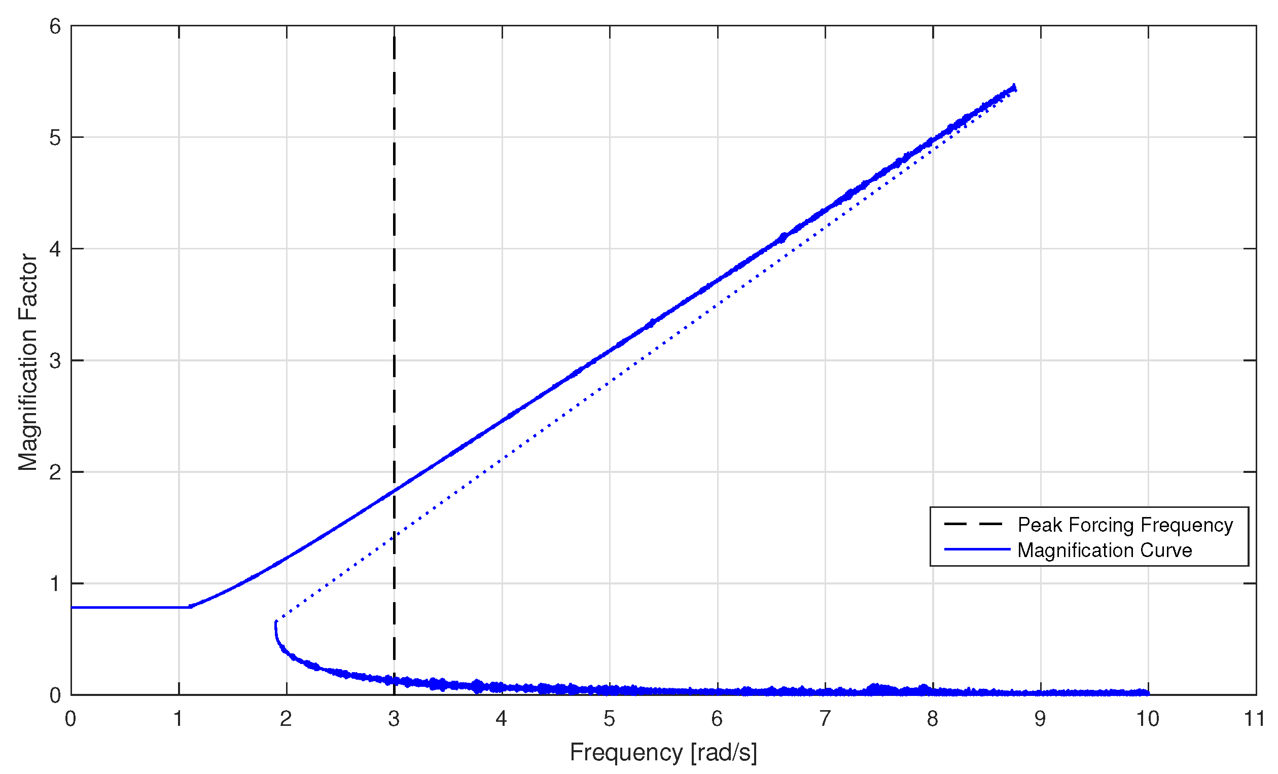
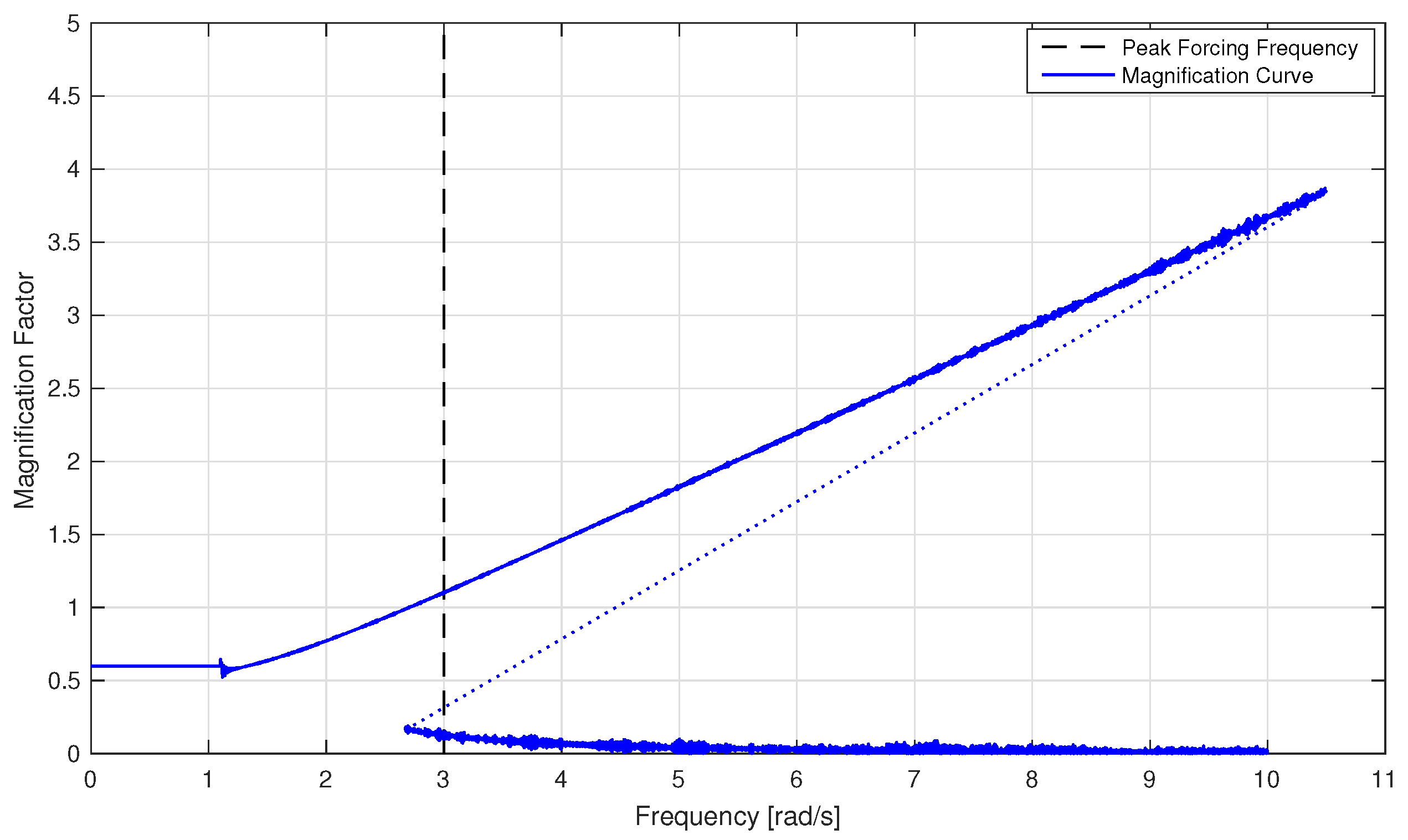
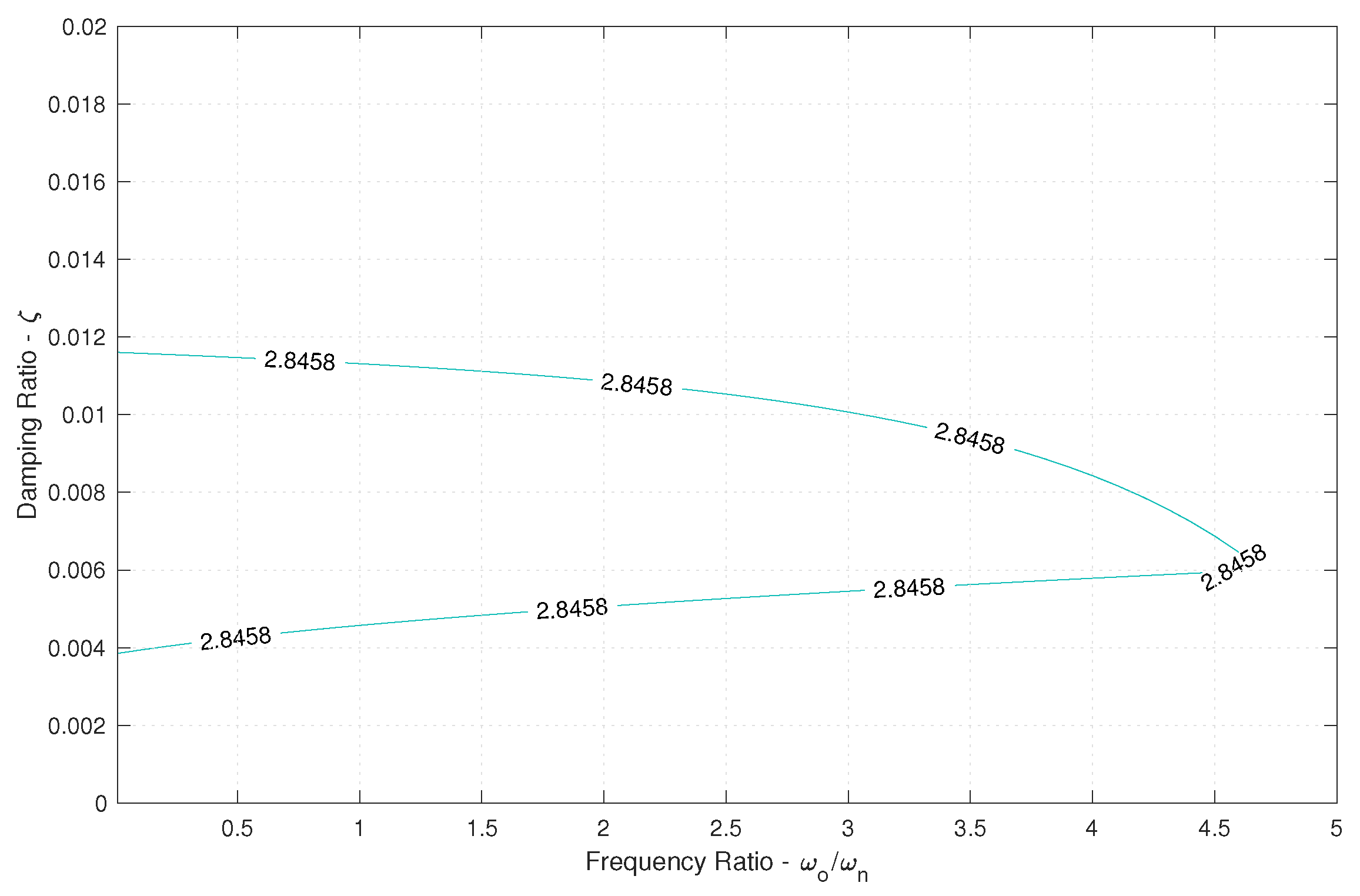
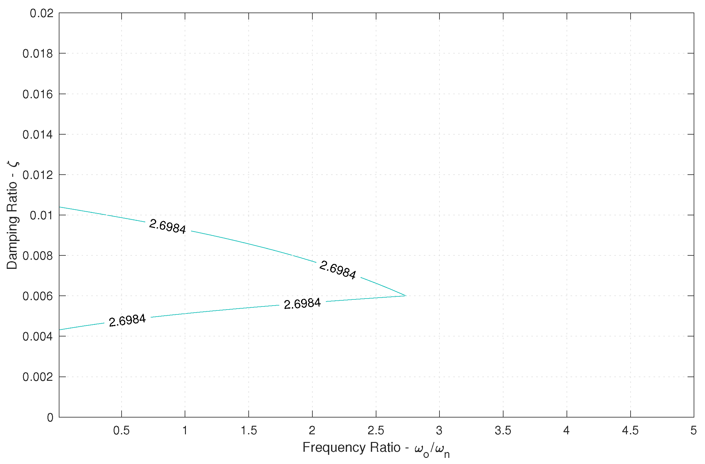
As seen in Figure 11, Figure 12 and Figure 13, increasing the forcing factor shifts the contour to the left. As the Duffing oscillators become more and more non-linear and non-stationary due to the increased forcing factor, there are fewer equivalent linear systems available to represent the Duffing oscillators. As such, the probability that there exists a linear system that shares inputs that lead to extremes with the non-linear system of interest decreases. The parameters from these contours are sampled such that about 20 sets of parameters were selected for input into the DLG for the purpose of simplicity and speed. Furthermore, the bulk of these sets of parameters fall near the bend in the contours, at frequency ratio values above 1.0. The majority of resulting natural frequencies fall below 1.0 rad/s, which may have an effect on the performance of the MUELS method due to the distance between the ELS natural frequencies and the peak forcing frequency. While it is possible that increasing this discretization, i.e., using more parameter sets from around the contour, would increase accuracy and performance, only around 20 parameter sets from each contour were used for this paper.

Table 3. The TEV for the given return period and the selected linear natural frequencies, ${\omega }_n$, and damping ratios, $\zeta$, for each forcing factor.

${\mathit{F}}_{\mathit{s}}$	TEV	${\mathit{\omega }}_{\mathit{n}\mathbf{,}\mathit{sel}}$	${\mathit{\zeta }}_{\mathit{sel}}$
10.0	4.793	0.059	0.006
14.7	4.774	0.196	0.009
17.0	4.761	0.148	0.006

outlines the TEV and selected parameters for each forcing factor. The parameter selection process is detailed in Section 2.4.

The linear natural frequencies and resulting transfer functions selected have little overlap with the energy from the input spectrum. Further investigations into the importance of prioritizing systems whose transfer functions overlap more with the input spectrum will be considered in future work.

One of the major benefits of the MUELS method is the increase in computational efficiency compared to Monte Carlo simulations. In this application, a single MUELS running for each forcing factor, including gathering training data and producing 1000 realizations, took 14,705 s on a quad-core processor. To produce 4000 Monte Carlo simulations for the same return period of 58 h took 144,840 s on eight cores. While there were more MCS produced, generating an equivalent number of MUELS realizations would add around 900 s per parameter set, or about 18,000 s for an entire MUELS run.

The current configuration of MUELS, which takes about 10–15% of the time of Monte Carlo simulations, allows for some increase in fidelity at the cost of computational effort. One area that could improve the accuracy of the MUELS method would be, as mentioned earlier, a finer discretization of the contour to examine more parameter sets.

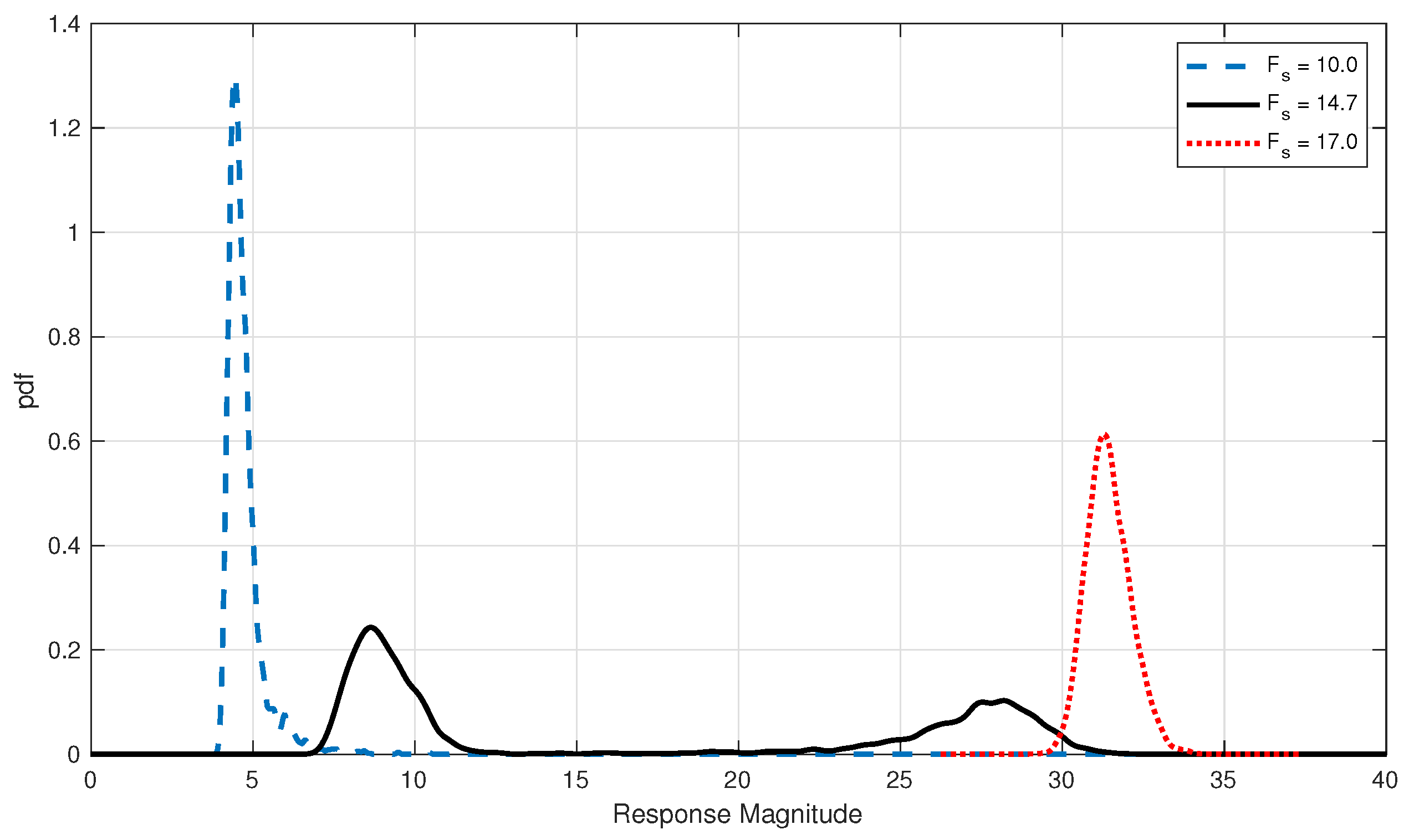
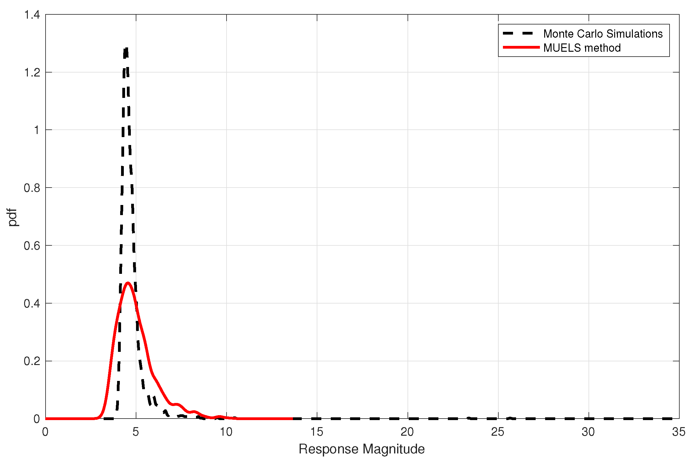
Figure 14, Figure 15 and Figure 16 show the selected MUELS extreme PDF and the extreme Monte Carlo PDF for each forcing factor. Note that each PDF was generated using a kernel density estimator.

In the $F_s=10.0$ case in Figure 14, the MUELS method extreme PDF predicted the most probable maximum of the Monte Carlo simulations well. The MUELS method PDF has a larger standard deviation than the MCS PDF but has a large amount of overlap and, therefore, valid extreme realizations.

The MUELS method was able to recover the two attractors in the $F_s=14.7$ case successfully. The under-prediction here could be the result of the TEV, given the levels of non-linearity that were introduced or since there are now essentially two return periods to examine: that of the small attractor and that of the large attractor. While the MUELS method does under-predict the MCS in the most probable maxima of both attractors, there is still a good amount of overlap that can provide valid extreme realizations.

In the $F_s=17.0$ case, the MUELS method retained some realizations that did not contain excursions. Furthermore, the amount of overlap between the MUELS method PDF and the Monte Carlo PDF is reduced even more.

The immediately evident and important characteristic of the $F_s=14.7$ PDF is the bi-modality, while the $F_s=10.0$ and $F_s=17.0$ cases exhibit uni-modality in the smaller domain of attraction and larger domain of attraction, respectively. The most obvious comparison we can make between the MCS and MUELS method is the x-value location of the peaks and the area of each of the peaks. It should be reiterated that each peak is representative of a different domain of attraction, as indicated in Section 2.2. As such, the area and the x-value of the maximum of each peak were used to compare the MUELS method with the Monte Carlo simulations.

Table 4. Comparison of pertinent PDF characteristics between the MUELS method and Monte Carlo simulations. The mean absolute percentage error (MAPE) between the MUELS method and MCS is also shown. Note that, for $F_s=10.0$ and $F_s=17.0$, there was only one attractor in the Monte Carlo simulations and, therefore, only one peak to compare.

	${\mathit{F}}_{\mathit{s}}\mathbf{=}\mathbf{10.0}$			${\mathit{F}}_{\mathit{s}}\mathbf{=}\mathbf{14.7}$			${\mathit{F}}_{\mathit{s}}\mathbf{=}\mathbf{17.0}$
Characteristic	MUELS	MCS	MAPE	MUELS	MCS	MAPE	MUELS	MCS	MAPE
Peak 1 X-Value	4.55	4.44	0.03	7.62	8.64	0.12	8.71	N/A	N/A
Attractor 1 Area	1.00	1.00	0.00	0.66	0.57	0.16	0.16	N/A	N/A
Peak 2 X-Value	N/A	N/A	N/A	25.02	28.19	0.11	25.52	31.29	0.18
Attractor 2 Area	N/A	N/A	N/A	0.34	0.43	0.21	0.84	1.00	0.16

shows the specified characteristics of the extreme MCS and MUELS PDFs and the mean absolute percentage error between the two.

There were a limited number of excursions in the $F_s=10.0$ Monte Carlo simulations, which is not reflected in the significant figures shown. That being said, the performance of the MUELS method for $F_s=10.0$ produced results nearly identical to MCS. This was expected, as the $F_s=10.0$ case is nearly linear, which resulted in a closer match between the ELS and the actual oscillator. While the MUELS PDF had more variance, as seen in Figure 14, this provides a solid foundation to produce an infinite number of extreme realizations at any return period of interest.

For $F_s=14.7$, the MUELS method under-predicts the MCS in both peak x-value and number of simulations with excursions. The under-prediction could be due to the MUELS method reaching the non-linearity limits or it could be due to the TEV selection. For this section, the TEV was determined simply by using the return period of 58.3 h and the zero-upcrossing period for each forcing factor. It is important to reiterate that the TEV becomes less meaningful as more non-linearity is introduced. The TEV is still a good starting point but cannot be expected to produce accurate results without any changes made to account for non-linearity.

For $F_s=17.0$, the MUELS method under-predicted the MCS again. In fact, there were a number of DLG inputs that did not result in an excursion in the 100-second realization. The under-prediction here is most likely the result of both TEV selection and reaching the non-linear limits of the MUELS method. Despite this, the large attractor x-value of the peak fell within 20% of the MCS most probable maximum and there are a number of realizations that overlap with the Monte Carlo extreme PDF. In practice, the amount of overlap would not be known, but schemes are being developed to form an acceptance–rejection method based on extreme value theory and knowledge of the system, which will enable one to estimate the amount of overlap between the true extreme value distribution and the extreme PDF from the MUELS method.

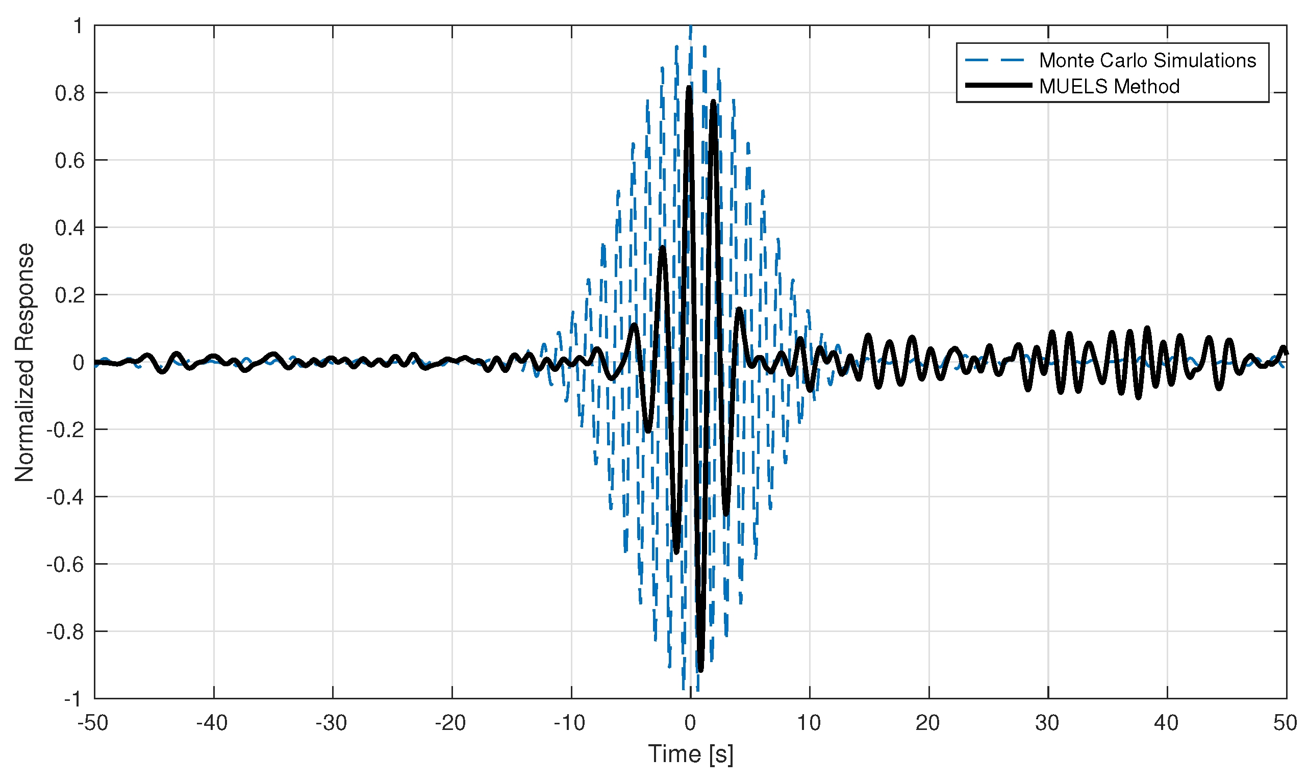
3.2. Time Series Comparison

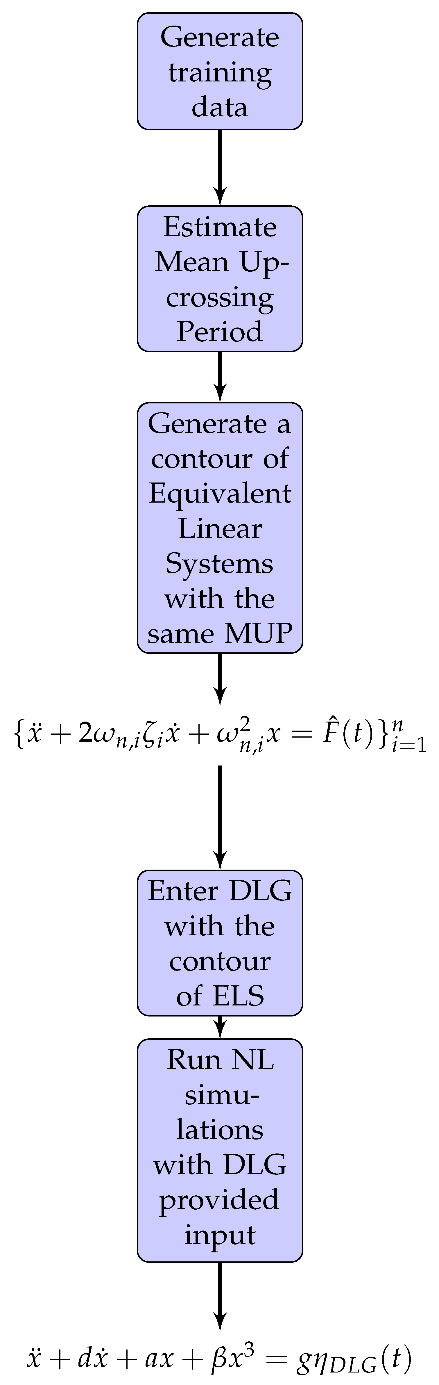
One of the major benefits of the MUELS method is the ability to produce any number of time series realizations that lead to an extreme response. It should be reiterated that the difference between just running Monte Carlo simulations and the MUELS method is that the MUELS method uses the DLG to produce multiple sets of input realizations from different equivalent linear systems of relatively short length. After the equivalent linear system parameters are selected, the DLG is capable of producing many realizations for that set of linear parameters that potentially lead to extremes in the non-linear system of interest. That being said, it is important to compare the MUELS method time series with Monte Carlo simulations to ensure that the time series have the similar characteristics near extremes. The phase sampling procedure in the DLG results in input time series that lead to linear extremes at $t=0$. Using the time series as input into the non-linear system will not necessarily result in an extreme or potential extreme at $t=0$ and that is reflected in the ensemble average time series. The lag is more noticeable when compared to the Monte Carlo simulation ensemble average near extremes, which was set to have the extreme at $t=0$, so the magnitudes were scaled and normalized to match the relationship between the peak value of the largest attractor for the Monte Carlo simulations and the MUELS method. 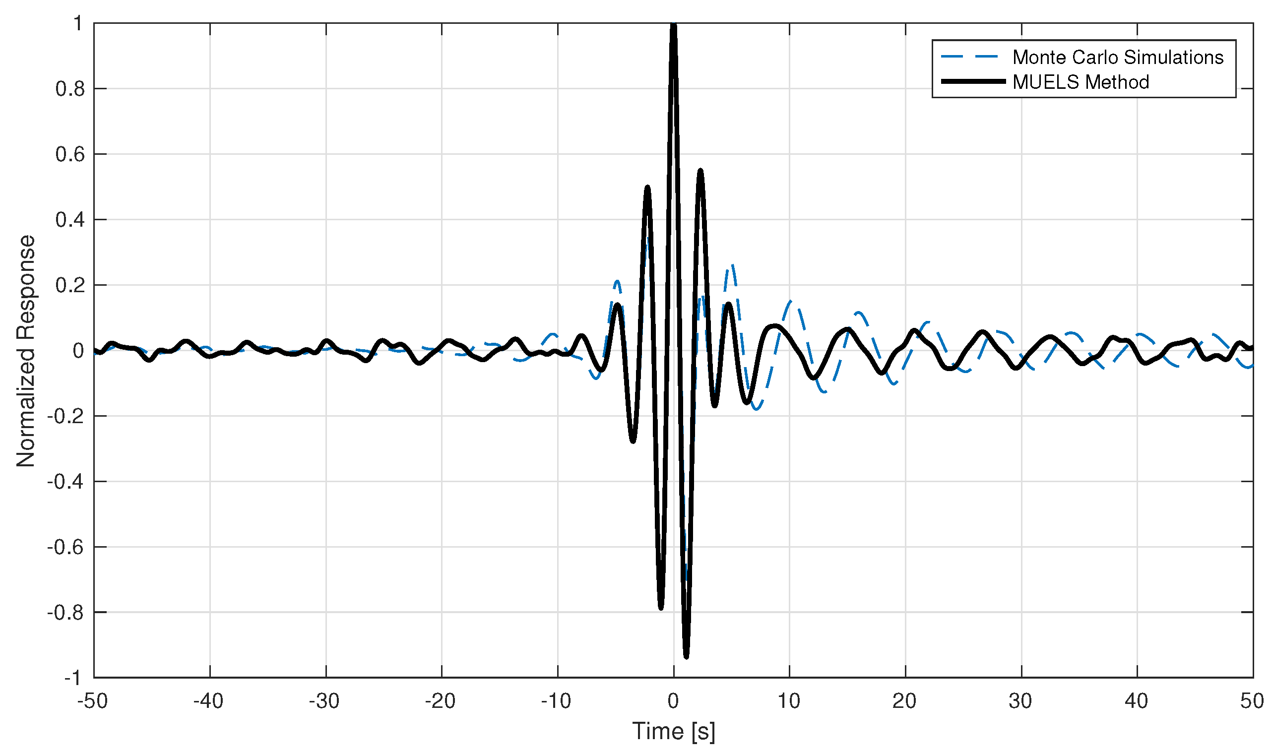Figure 17, Figure 18 and Figure 19 show these normalized ensemble averages near extremes for the Monte Carlo simulations and the MUELS method for each forcing factor.

In the $F_s=10.0$ case, the MUELS method and Monte Carlo simulations have very similar mean frequencies near $t=0$ and the magnitudes of the peaks leading up to the extreme value. Since the $F_s=10.0$ case is the most linear and, therefore, more immediately compatible with the DLG, it follows that it would produce time series that are closer to Monte Carlo simulations. It also seems to capture the dynamics shown in the Monte Carlo simulations further away from the extreme.

In the $F_s=14.7$ case, the MUELS method ensemble average seems to have a lower characteristic frequency than the Monte Carlo simulations. This may be a result of the lag mentioned earlier as the zero-upcrossing period should remain constant due to the fact that the input time series are valid realizations of the input spectrum. It is also interesting to note that the minimum value of the MUELS method after the positive peak follows the behavior of the Monte Carlo simulations while having a larger magnitude than the positive maximum of the MUELS method.

In the $F_s=17.0$ case, the MUELS method again has a lower characteristic frequency than the MUELS method. The buildup to the maximum is not as gradual or symmetric, as shown in the Monte Carlo ensemble average, but again re-centering the MUELS time series would reduce some of these deviations.

A future comparison between the MUELS method and Monte Carlo simulations would center the MUELS ensemble average to have a clearer comparison between the magnitudes of the ensemble average between the MCS and MUELS method. While the re-centering would improve the MUELS method performance relative to the Monte Carlo simulations, there may be another point of improvement in the TEV selection.

4. Conclusions

In this paper, the abilities and the limits of the MUELS method were tested. Three systems of varying non-linearity and non-stationarity were used to compare the MUELS method with the conventional method of Monte Carlo simulations. The key characteristic in each of the systems was the number of excursions into a domain of attraction with peak magnitudes two to three times larger than the base domain of attraction’s peaks. In general, the MUELS method under-predicted extreme characteristics found using Monte Carlo simulations but remained within about 20%. That being said, the computational expense of the MUELS method was only 10–15% of the Monte Carlo simulations on a less computationally powerful setup. The reduced load could allow for a larger number of potential surrogate linear systems for the MUELS method to test.

One of the major benefits of the MUELS method is the ability to produce time series realizations of conditional extremes. In comparing the ensemble average of the MUELS method and Monte Carlo simulations near extremes, it was found that there was a degradation in accuracy as non-linearity increased. One main cause of this is likely the fact that, while the DLG produces extreme linear time series with a maximum at $t=0$, there is no basis for those inputs to provide a non-linear realization with a maximum at exactly $t=0$. Additionally, a centering of the maximum values before taking the ensemble average would certainly improve both the ensemble average magnitude and average period when compared to Monte Carlo simulations.

Future studies into using alternative TEVs to minimize the distance between the MUELS method extreme PDF, the Monte Carlo simulations, and finer discretized parameter contours could potentially improve the MUELS method performance.

References

1. Gumbel, E. Statistics of Extremes; Echo Point Books and Media: Brattleboro, VT, USA, 1958. [Google Scholar]
2. Leadbetter, M.; Rootzen, H. Extermal Theory for Stochastic Processes. Ann. Probab. 1988, 16, 431–478. [Google Scholar] [CrossRef]
3. Grigoriu, M.; Samorodnitsky, G. Reliability of Dynamic Systems in Random Environment by Extreme Value Theory. Prob. Eng. Mech. 2014, 38, 54–69. [Google Scholar] [CrossRef]
4. Pipiras, V. Pitfalls of data-driven peaks-over-threshold analysis: Perspectives from extreme ship motions. Prob. Eng. Mech. 2020, 60, 103053. [Google Scholar] [CrossRef]
5. Belenky, V.; Glotzer, D.; Pipiras, V.; Sapsis, T. Distribution Tail Structure and Extreme Value Analysis of Constrained Piecewise Linear Oscillators. Prob. Eng. Mech. 2019, 57, 1–13. [Google Scholar] [CrossRef]
6. Zhang, Y.; Spanos, P. A Linearization Scheme for Vibrations due to Combined Deterministic and Stochastic Loads. Prob. Eng. Mech. 2020, 60, 103028. [Google Scholar] [CrossRef]
7. Jensen, J.; Choi, J.; Nielsen, U. Statistical Prediction of Parametric Roll using FORM. Ocean Eng. 2017, 144, 235–242. [Google Scholar] [CrossRef]
8. Kim, D. Design Loads Generator: Estimation of Extreme Environmental Loadings for Ship and Offshore Applications; University of Michigan: Ann Arbor, MI, USA, 2012. [Google Scholar]
9. Ochi, M. Applied Probability and Stochastic Processes; Wiley-Interscience: Hoboken, NJ, USA, 1990. [Google Scholar]
10. Seyffert, H.; Troesch, A.; Collette, M. Combined Stochastic Lateral and In-Plane Loading of a Stiffened Ship Panel Leading to Collapse. Marine Struct. 2019, 67, 102620. [Google Scholar] [CrossRef]
11. Edwards, S.; Troesch, A.; Collete, M. Estimating Extreme Characteristics of Stochastic Non-Linear Systems. Ocean Eng. 2021, 225, 109042. [Google Scholar] [CrossRef]
12. Det Norske Vertias. DNV-RP-C205 Environmental Conditions and Environmental Loads–Recommended Practice. 2010. Available online: https://www.dnv.com/oilgas/download/dnv-rp-c205-environmental-conditions-and-environmental-loads.html (accessed on 20 September 2023).
13. Namachchivaya, N. Stochastic Bifurcation. App. Math. Comp. 1990, 39, 101–159. [Google Scholar] [CrossRef]
Figure 1. An example pdf showing where the truncation point was placed for estimated statistics for the dominant attractor.
Engproc 39 00120 g001
Figure 2. The moving RMS of an example Duffing oscillator compared with the threshold and the average RMS of the dominant attractor.
Engproc 39 00120 g002
Figure 3. An example stationarity test for F s = 10.0 . Note that there are no excursions in this example.
Engproc 39 00120 g003
Figure 4. An example stationarity test for F s = 14.7 . Note that there is a single excursion in this example.
Engproc 39 00120 g004
Figure 5. An example stationarity test for F s = 17.0 . Note that are 19 discrete excursions in this example.
Engproc 39 00120 g005
Figure 6. Magnification curve for F s = 10.0 along with the peak forcing frequency. Note that the dotted line is an unstable branch.
Engproc 39 00120 g006
Figure 7. Magnification curve for F s = 14.7 along with the peak forcing frequency. Note that the dotted line is an unstable branch.
Engproc 39 00120 g007
Figure 8. Magnification curve for F s = 17.0 along with the peak forcing frequency. Note that the dotted line is an unstable branch.
Engproc 39 00120 g008
Figure 9. Kernel density estimated probability density functions for the largest value in a 58-h long time series for each forcing factor.
Engproc 39 00120 g009
Figure 10. The Matched Upcrossing Equivalent Linear System (MUELS) method flowchart.
Engproc 39 00120 g010
Figure 11. The equivalent linear system contour for F s = 10.0 along with the zero-upcrossing frequency of 2.8458 rad/s. Note that ω o is the peak frequency of the input spectrum and ω n is the linear natural frequency.
Engproc 39 00120 g011
Figure 12. The equivalent linear system contour for F s = 14.7 along with the zero-upcrossing frequency of 2.6984 rad/s. Note that ω o is the peak frequency of the input spectrum and ω n is the linear natural frequency.
Engproc 39 00120 g012
Figure 13. The equivalent linear system contour for F s = 17.0 along with the zero-upcrossing frequency of 2.5850 rad/s. Note that ω o is the peak frequency of the input spectrum and ω n is the linear natural frequency.
Engproc 39 00120 g013
Figure 14. The extreme value PDF for the Monte Carlo simulations and the selected extreme value distribution for the MUELS method for F s = 10.0 .
Engproc 39 00120 g014
Figure 15. The extreme value PDF for the Monte Carlo simulations and the selected extreme value distribution for the MUELS method for F s = 14.7 .
Engproc 39 00120 g015
Figure 16. The extreme value PDF for the Monte Carlo simulations and the selected extreme value distribution for the MUELS method for F s = 17.0 .
Engproc 39 00120 g016
Figure 17. Ensemble average of the time series near extremes for Monte Carlo simulations and the MUELS method for F s = 10.0 . Note that the MUELS method results are not centered.
Engproc 39 00120 g017
Figure 18. Ensemble average of the time series near extremes for Monte Carlo simulations and the MUELS method for F s = 14.7 . Note that the MUELS method results are not centered.
Engproc 39 00120 g018
Figure 19. Ensemble average of the time series near extremes for Monte Carlo simulations and the MUELS method for F s = 17.0 . Note that the MUELS method results are not centered.
Engproc 39 00120 g019