Abstract
To achieve accurate position tracking, there is a need to develop high-fidelity robot arm models that are compliant and affordable. However, physics-based models are constrained by their stiffness and complexity. Therefore, reduced-order modelling developed from data through sub-space system identification is proposed as a solution to this problem. A high-fidelity simulation model of a two-link robot arm developed in MATLAB and Simulink was used to generate synthetic data, and the data acquired was used for the estimation and validation of first- and second-order linear state-space models. Due to its effective tracking characteristics, the model predictive control technique was used for trajectory tracking. The results of the simulations demonstrate that the first-order and second-order models can track the intended set points accurately but at the cost of larger joint torques required to counteract gravity. The results show that low-order and data-compliant models can follow trajectories with high precision. MATLAB 2020a was used for all simulations.
1. Introduction
Subspace system identification is a class of techniques for estimating state space models based on low-rank qualities of certain observability/prediction sets [1,2]. One significant benefit of subspace system identification is that it does not distinguish between standard single-input single-output identification and multi-input, multi-output system identification, where the input and output are vectors. In contrast, with methods like prediction error, selecting model structures and appropriate parameterizations is crucial. The methods’ reliance on reliable numerical techniques, avoidance of optimization issues and potential local minima are further benefits of subspace identification [3].
In robotic manipulation, high-precision trajectory tracking is essential. Industrial robots deal with this by using high-performance hardware technology that is stiff but compliant. However, economic robots need sophisticated control to ensure precise position tracking. Many works of literature have extensively examined model-based control of robotic arms, including control in joint and task space [4,5,6,7,8,9,10,11,12]. Due to their potential to improve control performance in comparison to conventional control approaches and potentially allow the use of affordable hardware or compliant robots in tasks where high-precision trajectory tracking is required, data-driven models for controller design applied to robotic manipulation have attracted increasing interest in recent years. Data-driven techniques can effectively incorporate prior model knowledge [13]. Modeling and control of low-cost robots that can achieve great tracking accuracy without sacrificing overall performance and efficiency is still an open area of research.
In this study, we provide a subspace identification technique for estimating and validating a low-order, data-compliant, and cost-effective two-link robot arm for precise position control. A high-fidelity simulation model in [14] was used to generate synthetic data, and its implementation is reported in [15]. Accurate trajectory tracking performance is achieved using a model predictive control (MPC) strategy. The challenge of achieving high-precision trajectory tracking can be surmounted by combining data-driven models with MPC. MPC allows for optimal operation while satisfying constraints, while data-driven algorithms improve system performance and capacity to adapt to system changes [16,17].
The outline of the rest of the paper is as follows: Section 2 explains the materials and methods, which include the dynamic model of a two-link robot, feedback linearization of the robot arm, the concept of sub-space-based system identification and the model predictive controller. Simulation results are presented in Section 3, while Section 4 concludes the paper.
2. Materials and Methods
2.1. Dynamic Model of a Two-Link Robot Arm
A two-link planar manipulator with revolute joints is shown in Figure 1 below.
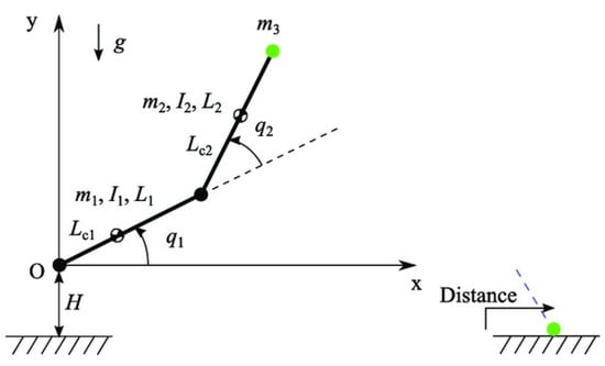
Figure 1.
A two-link planar manipulator with revolute joints [18].
The Euler-Lagrange formulation is used to calculate the dynamics of the robot arm in terms of stored potential and kinetic energies in the system. The modeling assumptions are as follows:
Given the inertial tensors, the kinetic energy of the first and second links are derived as follows:
Potential energy for the first and second links are given as:
where, is the gravitational constant.
The Lagrangian equation is given as follows:
where and .
The Lagrange equations are expressed by:
For two-link arm, = 1, 2
Therefore,
The matrix representation:
The Lagrange equation can be rewritten as:
where, is the inertial matrix, is the Coriolis and Centrifugal terms, is the gravity term, is the torque or force vector.
Feedback Linearization of the Two-Link Robot Arm
From Equation (16), the link equation can be re-written as:
Substituting into Equation (18) gives:
Equation (20) is now in the form of the general feedback linearization expression given as:
where, is an identity matrix.
Linearizing around a stationary point, the Coriolis and Centrifugal forces/terms will disappear because they are quadratic in the angular velocity, that is, .
The parameters of the linearized model can be derived thus:
Table 1 shows the parameter values of the linearized two-link robot arm model.

Table 1.
The parameter values of the linearized two-link robot arm model.
2.2. Sub-Space-Based System Identification
Consider a multi-input multi-output (MIMO) controllable systems where denotes the vector of constrained manipulated variables, taking values in a nonempty convex subset , where denote the lower and upper bounds of the input variables, and denotes the vector of measured output variables. is piecewise constant and defined over an arbitrary sampling instance as:
where is the sampling time and and denote state and output at the sample time.
The system matrices for a discrete-time linear time-invariant (LTI) system take the following form:
where and denote the vectors of the state variables and measured outputs, and and are zero mean white vectors of process noise and measurement noise with the following covariance matrices:
where , , and , are covariance matrices, and is the Kronecker delta function. The subspace-based system identification techniques utilize Hankel matrices constructed by stacking the output measurements and manipulated variables as follows:
where is a user-specified parameter that limits the maximum order of the system , and, is determined by the number of sample times of data. By using the previous equation, the past and future Hankel matrices for input and output are defined:
Similar block-Hankel matrices are made for process and measurement noises and are defined in a similar way. The state sequences are defined as follows:
Furthermore, these matrices are used in the algorithm:
By recursive substitution into the state space model equations, it is straightforward to show:
where:
Therefore and can be calculated by decomposition methods [20].
2.3. Linear Model Predictive Controller
Model Predictive Control (MPC) is an advanced algorithm that utilizes the dynamic model of the process to predict its future behaviour over a finite time horizon and compute an optimal control input that minimizes the cost function while satisfying the system constraint. It can be mathematically represented below:
According to the receding horizon concept, the optimal sequence is over N steps, while the first optimal control action u*(t) is used. New measurements/state estimates are gotten at time t + 1, and the process of optimization is repeated [21].
3. Results and Discussions
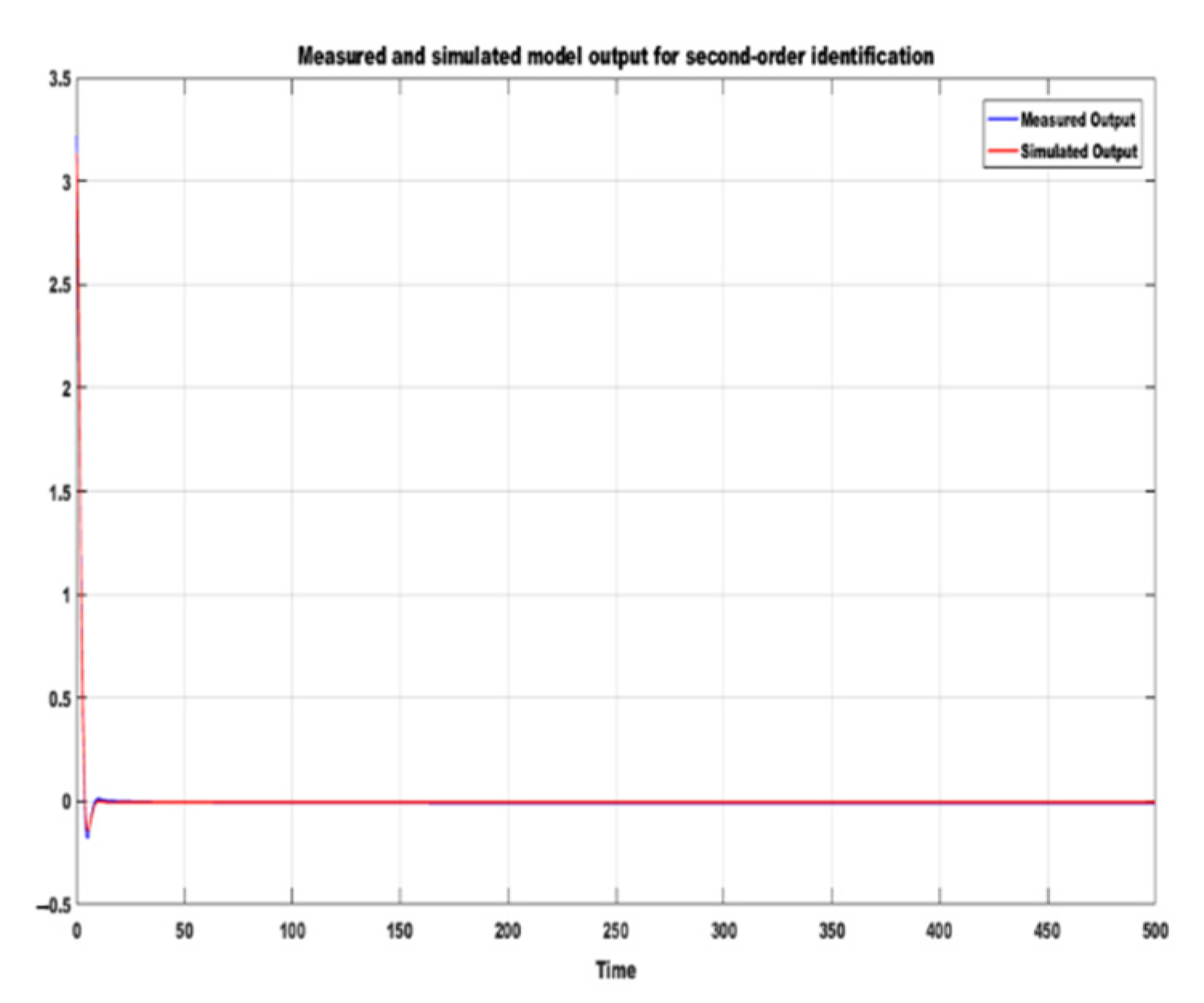
Figure 2 and Figure 3 show the fit of the model outputs between the estimation data and the validation data. Twenty-thousand-and-one samples of synthetic data were derived by simulating the two-link robot arm model in Simulink. The means of the data were removed. The whole sample was used as estimation data, while 50% of the sample (10,000) was used as validation data. The best fit for the first-order model is 85.08%, the final prediction error (FPE) is 9.671 × 10⁻²³, and the mean square error (MSE) is 0.0005915, using simulation focus. Likewise, the best fit for the second-order model is 96.34%, the final prediction error (FPE) is −3.561 × 10⁻²⁸, and the mean square error (MSE) is 4.614 × 10⁻⁵, using simulation focus. It can be observed from Figure 2 and Figure 3 that the higher the model order, the lower the FPE and MSE and the better the fit that can be achieved between the measured and the simulation output. However, overfitting must be avoided to achieve a reliable model identification.
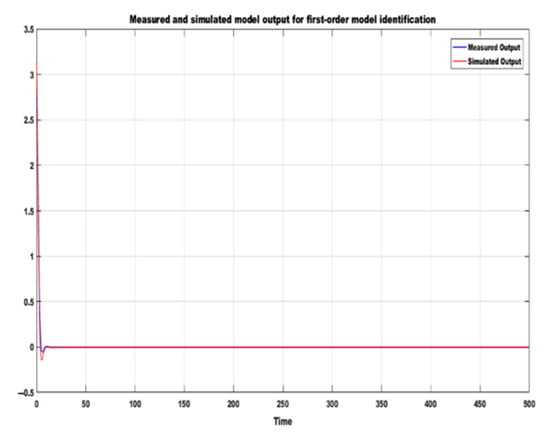
Figure 2.
Response of first order model identification.
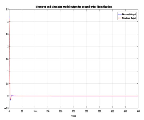
Figure 3.
Response of second order model identification.
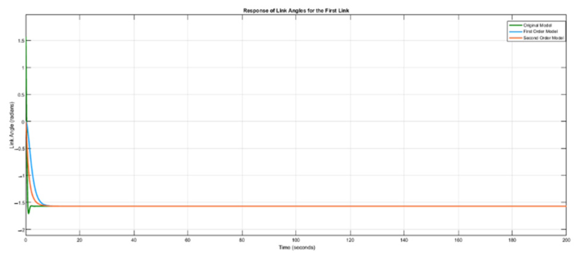
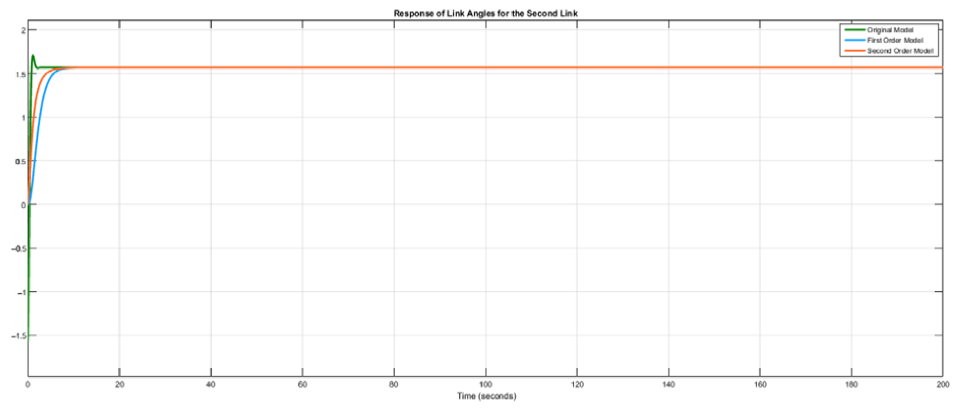
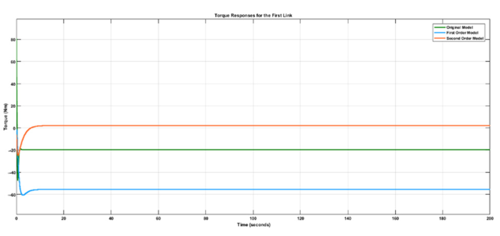
Figure 4, Figure 5, Figure 6 and Figure 7 show the simulation results of the outputs (link angles) and inputs (joint torques) of the original model, the first-order identified model and the second-order identified model. The MPC design parameters for achieving the trajectory-tracking of the identified models are: , , , and . The reference trajectories used for the identified model are the same as those used in the original model, which are and .
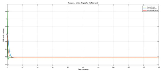
Figure 4.
Response of link angles for first link for .
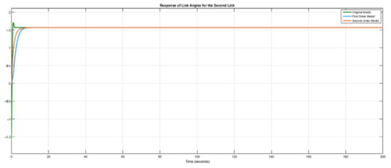
Figure 5.
Response of link angles for first link for .
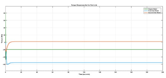
Figure 6.
Response of joint torques for the first link.
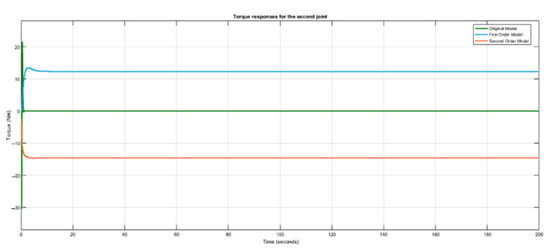
Figure 7.
Response of joint torques for the second link.
Figure 4 and Figure 5 show that the first-order and the second-order identified model were able to track the reference, just like the original model. However, the second-order model settled faster than the first-order model due to its better modelling accuracy. But in a situation whereby a low-order system is a priority, the first-order model is sufficient to accomplish the trajectory tracking task.
Figure 6 shows that the torque required to achieve the trajectory tracking at the first joint for the second-order identified model was larger than the torque required to achieve the same goal for the first-order identified model. The original model also had a higher initial torque response of 80 Nm. This results from the higher model order of the original model and the second-order identified model, which require more actuation effort than the first-order identified model with only one state. Also, since the effect of gravity is usually more pronounced at the first link, the torque required to maintain the link against the force of gravity tends to increase with the number of states of the system.
From Figure 7 it can be observed that the torque required to achieve the trajectory tracking at the second joint for the second-order identified model is the smallest when compared to the torque responses of the original model and the first-order model. The first-order model has the highest torque at this joint. These responses are in accordance with the fact that, at the second joint, the effect of gravity is less pronounced. That is why it can be observed from the response of the original model that the highest peak of the torque was a little above 20 Nm compared with the first link with a peak of 80 Nm. Therefore, more torque will be needed at this joint to maintain the stability of the second link if the system state(s) is low. Hence, this joint’s first-order identified model possesses the highest torque response.
4. Conclusions
A data-driven model of a two-link robot arm using sub-space system identification is presented. Synthetic data was generated from a high-fidelity simulation model developed in MATLAB and Simulink, and the acquired data was used for model estimation and validation of first- and second-order linear state-space models. The model predictive control strategy was employed for trajectory tracking due to its good tracking characteristics. It was deduced that the first-order model could achieve trajectory tracking of the desired set-point, but a higher toque will be required at the second joint to maintain the stability of the second link of the robotic manipulator. Furthermore, it was discovered that the second-order model also achieved good tracking performance but required higher actuator work by the input torque at the first joint to cope with the effect of gravity. Finally, the original model had an initial spike of 80 Nm at the first joint due to more actuator work required to cope with the effect of gravity but had a reduced spike of 20 Nm at the second joint due to less actuator work at the joint, since the effect of gravity is less pronounced at the second link. Any of the data-driven models may be used for trajectory tracking applications such as welding, machining, laser cutting, surgery, et cetera when the robot arm model is not available or is too complex to model mathematically since they also exhibit high trajectory tracking performance characteristics when compared with the original model. Finally, data-based robot arm modelling and control provide an opportunity to design a low-order system that can achieve the goal of accurate trajectory tracking when the number of states of the real system is too large, thereby reducing cost. Non-linear model identification and control will be the main topics of future research.
Supplementary Materials
The presentation materials can be downloaded at: https://www.mdpi.com/article/10.3390/ECP2023-14698/s1.
Author Contributions
Conceptualization, A.T.B.; methodology, A.T.B. and E.E.C.I.; software, A.T.B.; supervision, M.B.M. All authors have read and agreed to the published version of the manuscript.
Funding
This research received no external funding.
Institutional Review Board Statement
Not applicable.
Data Availability Statement
Not applicable.
Acknowledgments
The constructive criticisms of the computer and control group of Ahmadu Bello University are gratefully acknowledged.
Conflicts of Interest
The authors declare no conflict of interest.
References
- Wahlberg, B.; Jansson, M.; Matsko, T.; Molander, M.A. Experiences from Subspace Identification—Comments from Process Industry Users and Researchers. Available online: Diva-portal.org/smash/get/diva2:384792/FULLTEXT01.pdf (accessed on 15 February 2023).
- Palanthandalam-Madapusi, H.J.; Lacy, S.; Hoagg, J.B.; Bernstein, D.S. Subspace-Based Identification for Linear and Nonlinear Systems. In Proceedings of the 2005, American Control Conference, Portland, OR, USA, 8–10 June 2005. [Google Scholar]
- Ljung, L. System Identification Toolbox User’s Guide. 1988–2022. Available online: https://www.mathworks.com/ident (accessed on 17 February 2023).
- Baccouch, M.; Dodds, S. A Two-Link Robot Manipulator: Simulation and Control Design. Int. J. Robot. Eng. 2020, 5, 1–17. [Google Scholar] [CrossRef]
- Nguyen, T. Sliding Mode Control-Based System for the Two-Link Robot Arm. Int. J. Electr. Comput. Eng. 2019, 9, 2771–2778. [Google Scholar] [CrossRef]
- Nguyen, T. Fractional-Order Sliding Mode Controller for the Two-Link Robot Arm. Int. J. Electr. Comput. Eng. 2020, 10, 5579–5585. [Google Scholar] [CrossRef]
- Kharabian, B.; Mirinejad, H. Hybrid Sliding Mode/H-Infinity Control Approach for Uncertain Flexible Manipulators. IEEE Access 2020, 8, 170452–170460. [Google Scholar] [CrossRef]
- Ezkeziyaw, A. Model Predictive Controller Design for Seed Sowing Row Planting Agricultural Robot. Master’s Thesis, Bahir Dar Institute of Technology, Bahir Dar, Ethiopia, 2022. [Google Scholar]
- Trung, T.V.; Iwasaki, M. Fast and Precise Positioning with Coupling Torque Compensation for a Flexible Lightweight Two-Link Manipulator with Elastic Joints. In IEEE/ASME Transactions on Mechatronics; IEEE: Piscataway, NJ, USA, 2022; pp. 1–12. [Google Scholar]
- Khemaissia, S.; Soufi, Y. A Biologically inspired Adaptive Model Theory for Humanoid Robot Arm Control. In Proceedings of the 2022 IEEE 2nd International Maghreb Meeting of the Conference on Sciences and Techniques of Automatic Control and Computer Engineering (MI-STA), Sabratha, Libya, 23–25 May 2022; pp. 193–198. [Google Scholar]
- Kuo, Y.; Pongpanyaporn, P. Continuous-Time Nonlinear Model Predictive Tracking Control with Input Constraints using Feedback Linearization. Appl. Sci. 2022, 12, 5016. [Google Scholar] [CrossRef]
- Bettega, J.; Richiedie, D. Trajectory Tracking in an Under-Actuated Non-Minimum Phase Two-Link Multibody System through Model Predictive Control with Embedded Reference Dynamics. Mech. Mach. Theory 2023, 180, 105165. [Google Scholar] [CrossRef]
- Carron, A.; Arcari, E.; Wermelinger, M.; Hewing, L.; Hutter, M.; Zeilinger, M.N. Data-Driven Model Predictive Control for Trajectory Tracking with a Robotic Arm. IEEE Robot. Autom. Lett. 2019, 4, 3758–3765. [Google Scholar] [CrossRef]
- Sepahvand, S. Model Predictive Control of a Two-Link Robot Arm. MATLAB Central File Exchange. Available online: https://www.mathworks.com/matlabcentral/fileexchange/99729-model-predictive-control-of-a-two-link-robot-arm (accessed on 15 January 2023).
- Guechi, E.H.; Bouzoualegh, S.; Messikh, L.; Blazic, S. Model Predictive Control of a Two-Link Robot Arm. In Proceedings of the 2018 International Conference on Advanced Systems and Electric Technologies (IC_ASET), Hammamet, Tunisia, 22–25 March 2018; pp. 409–414. [Google Scholar]
- Sha’aban, Y.A. Automatic Tuning of MPC using Genetic Algorithm with Historic Process Data. In Proceedings of the 2022 IEEE 18th International Colloquium on Signal Processing & Applications (CSPA), Selangor, Malaysia, 12 May 2022; pp. 329–334. [Google Scholar]
- Marschik, C.; Roland, W.; Low-Baselli, B.; Steinbichler, G. Application of Hybrid Modelling in Polymer Processing. In Proceedings of the ANTEC 2020: The Annual Technical Conference for Plastic Professionals, Virtual, 30 March–5 May 2020; Available online: https://www.researchgate.net/profile/Christian-Marschik/publication/350649155_APPLICATION_OF_HYBRID_MODELING_IN_POLYMER_PROCESSING/links/606c047992851c91b1a6de2b/APPLICATION-OF-HYBRID-MODELING-IN-POLYMER-PROCESSING.pdf (accessed on 23 January 2023).
- Huang, Y.J. Variable Structure Control for a Two-link Robot Arm. Electr. Eng. 2003, 85, 195–204. [Google Scholar] [CrossRef]
- Bankole, A.T.; Igbonoba, E.E.C. A Novel Hybrid Proportional Derivative/H-Infinity Controller Design for Improved Trajectory Tracking of a Two-Link Robot Arm. 2022. Available online: https://www.researchsquare.com/article/re-2193905/v1.pdf (accessed on 30 January 2023).
- Kheradmandi, M. Data Driven Economic Model Predictive Control. Mathematics 2018, 6, 51. [Google Scholar] [CrossRef]
- Ellis, M.; Liu, J.; Christofides, P.D. Economic Model Predictive Control: Theory, Formulations and Chemical Process Applications; Springer: Berlin/Heidelberg, Germany, 2017. [Google Scholar]
Disclaimer/Publisher’s Note: The statements, opinions and data contained in all publications are solely those of the individual author(s) and contributor(s) and not of MDPI and/or the editor(s). MDPI and/or the editor(s) disclaim responsibility for any injury to people or property resulting from any ideas, methods, instructions or products referred to in the content. |
© 2023 by the authors. Licensee MDPI, Basel, Switzerland. This article is an open access article distributed under the terms and conditions of the Creative Commons Attribution (CC BY) license (https://creativecommons.org/licenses/by/4.0/).


