Design and Simulation of a Low-Power and High-Speed Fast Fourier Transform for Medical Image Compression ^†

Abstract

For front-end wireless applications in small battery-powered devices, discrete Fourier transform (DFT) is a critical processing method for discrete time signals. Advanced radix structures are created to reduce the impact of transistor malfunction. To develop DFT, with radix sizes 4, 8, etc., is a complex and tricky issue for algorithm designers. The main reason for this is that the butterfly algorithm’s lower-radix-level equations were manually estimated. This requires the selection of a new design process. As a result of fewer calculations and smaller memory requirements for computationally intensive scientific applications, this research focuses on the radix-4 fast Fourier-transform (FFT) technique. A new 64-point DFT method based on radix-4 FFT and multi-stage strategy to solve DFT-related issues is presented in this paper. Based on the results of simulations with Xilinx ISE, it can be concluded that the algorithm developed is faster than conventional approaches, with an 18.963 ns delay and 12.68 mW of power consumption. It was found that the computed picture compression drop ratios of 0.10, 0.31, 0.61 and 0.83 had a direct relationship to the varied tolerances tested, 0.0007625, 0.003246, 0.013075 and 0.03924. Fast reconstruction techniques, wireless medical devices and other applications benefit from this FFT’s low power consumption, small storage requirements, and high processing speed.

1. Introduction

One of the most widely utilized mathematical operations is fast Fourier transform. Several medical applications use fast Fourier transform for image reconstruction and frequency domain analysis. Image processing applications, such as filtering, compression, and de-noising, all rely on FFT to a certain extent. FFT, is used as an improved version of the traditional discrete signal processing tool (discrete Fourier transform), for medical image compression with various drop ratios. FFT is widely used in medical imaging, engineering, communication, and other fields because it transitions quickly from the T-domain to the F-domain and vice versa [1,2,3,4,5,6].

The medical imaging method provides images of the human body and its components for clinical application. Computer tomography (CT), magnetic resonance imaging (MRI), ultrasound and optical imaging technology are the most prevalent modes of medical imaging that produce a prohibitive amount of data. The images produced by these instruments are pixels representing the operations of human organs in terms of their visual depiction. They are also the patient’s most vital information and demand high storage and transmission width [7,8].

FFT-based compression is a compression algorithm, which can process the image quickly coupled with the transformed domain compression. The modified domain includes coefficients of both low and high frequencies that are measured. Various quantified coefficient values of high frequency are unimportant and almost equivalent to zero and remove them from the modified image. This pre-processing step leads to the compression platform. By supplying different symbols, the FFT method accomplishes compression. The majority of appearing symbols are assigned to be shorter while the rest are assigned to longer-size symbols. The variable-length compressed data are subsequently stored on transmission media.

As hospitals are progressing into digitization, filmless imaging and telemedicine, medical imagery becomes significantly important in the health sector. This has led to the major difficulty of developing compression algorithms that prevent diagnostic errors and have a high compression ratio for lower bandwidth and storage. In the medical area, particularly, quick diagnosis is only achievable when the required diagnostic information is maintained through the compression approach. These images help physicians to easily diagnose the inner parts of the body. They also help to perform keyhole procedures without too many incisions to reach the inner sections of the body. They can be processed quickly, analyzed objectively and made available in numerous places simultaneously by means of communication protocols and networks, such as digital imaging and communications in medicine (DICOM) protocol and picture archiving and communication system (PACS) networks, respectively. The X-ray, CT, MRI or ultrasound images contain huge amounts of data that demand vast channels or storage capacities. The implementation costs limit the storage capacity, even with the progress in storage capacity and connectivity [8,9,10]. There are certain approaches that create imperceptible variations and acceptable fidelity that can lead to medical picture low-loss compression. In this article, FFT-based compression is proposed.

Many different mathematical FFT algorithms vary from easy theories of complex numbers arithmetically to group and numerical theory; this paper provides an available technical outline and few characteristics while explaining the algorithms in the subsidiary sections. The DFT is obtained via the decomposition of a series of values into various frequency components, as given in Equations (1) and (2). This operation is useful in several fields, but it is always too slow to be practical for computing it directly from the given description.

$$X\left(k\right)=\sum _{n=0}^{N-1}x\left(n\right)e^{-j\left(\frac{2\pi }{N}\right)kn},\hspace{1em}0\le k\le N-1$$

(1)

$$x\left(n\right)=1/N\sum _{k=0}^{N-1}X(k)e^{j\left(\frac{2\pi }{N}\right)kn};\hspace{1em}0\le n\le N-1$$

(2)

The FFT is one of the new ways to calculate similar results faster: DFT takes N² arithmetical multiplications and N² − N addition operations (O(4N²), real multiplications and O(N(4N − 2) real additions) to naively compute the DFT of N-points. The speed difference may be huge, especially in long data sets where N may be higher. FFT can compute the DFT for $\frac{N}{2}{\log }_{r}N$ multiplications and $N{\log }_{r}N$ additions corresponding operation alone using twiddle factor W_N = e^−j2π/N [4,6] since it is using a butterfly operation and computes p ± αq (results six real adds and four real multiplications). As FFTs are staged algorithms, there are ${log}_2^N$ stages, and each stage has N/2 butterflies, so there should be four.

$$\begin{gathered} \mathrm{N}/2\times {log}_2^N=2\mathrm{N}\times {log}_2^N \mathrm{real} \mathrm{multiplications} \mathrm{and} 3\mathrm{N}\times {log}_2^N \mathrm{real} \\ \mathrm{additions} \mathrm{for} \text{N-point} \mathrm{DFT} \mathrm{through} \mathrm{FFT} \end{gathered}$$

(3a)

(Optimization is still possible, but these are basic equations).

N² and N(N−1) multiplications and additions in a normal DFT for N-point

(3b)

DFT estimation was practical due to these huge changes. For a broad range of applications, FFTs are of great importance—from DSP to algorithms for quick multiplication of high integer range [10,11]. From Equations (3a) and (3b), the cost estimation is given in

Table 1. Cost estimation of DFT and FFT.

N	DFT		FFT (Radix 2) (Optimized)		Speed Factor Improvement
	4N2	N(4N−2)	$2\mathbf{N}{\mathit{l}\mathit{o}\mathit{g}}_2^{\mathit{N}}$	$3\mathbf{N}{\mathit{l}\mathit{o}\mathit{g}}_2^{\mathit{N}}$	Multiplications	Additions
2	16	12	4	6	4	2
32	4096	4032	320	480	12.8	8.3
64	16,384	16,256	768	1152	21.333	14.11
1024	41,94,304	41,92,256	20,480	30,720	204.8	136.466

.

From Table 1, it is evident that FFT is less computationally intensive than DFT. When comparing the two methods, FFT is faster. It is important to note that, because FFTs are radix algorithms, this work shows that making minor changes to the algorithm in the order 2 results in faster FFT times. A DIT-FFT algorithm decomposes a signal based on the time sequence ‘x(n)’. Another categorization is the decimation-in-frequency FFT (DIF-FFT) algorithm, which decomposes using the frequency sequence ‘X(k)’. Radices are the foundation of these algorithms. Many intermediate results and memory locations are re-used in these algorithms, which makes them more efficient in the long run. These computational approaches happen with the help of butterflies called radix-2 butterflies.

In DIT-FFT, the inputs are arranged in bit reversal/normal order, and outputs are obtained in a normal order/bit reversal. The radix-2 DIT-FFT algorithm is a staged algorithm. The effective functioning of radix-2 depends on stages, butterflies, etc. Each stage has block(s), and each block has butterflies. These can be defined as follows, radix-2 algorithm consists of log₂N stages, and each stage consists of N/2^stage blocks, and each block consists of 2^stage−1 butterflies. As in signal processing (digital), most of the required arithmetic computations are additions and multiplications, radix-2 offers N/2 × log₂ N complex multiplications and N × log₂ N complex additions [9,10,11,12,13,14].

The radix-4 is an additional fast Fourier transform algorithm (FFT) that can be obtained by moving the base from 2 to 4. The power/index diminishes in direct proportion to the size of the base. There are 50% fewer stages in radix-4 than in radix-2 since N = 4M, indicating that stages have decreased by 50%. It is explained in more detail in the later sections on how radix-4 simplifies difficult calculations [15].

For computing sequences, the radix-4 algorithm is comparable to the radix-2 technique in terms of type and speed management. It takes place as follows: the given sequence divides into four parts based on ‘n’: The given sequence layout in radix-4 is as follows:

n = [0, 4, 8,… N − 4] results × (4n),

n = [1, 5, 9,… N − 3] results × (4n + 1),

n = [2, 6, 10,… N − 2] results × (4n + 2),

n = [3, 7, 11,… N − 1] results × (4n + 3) [16,17,18].

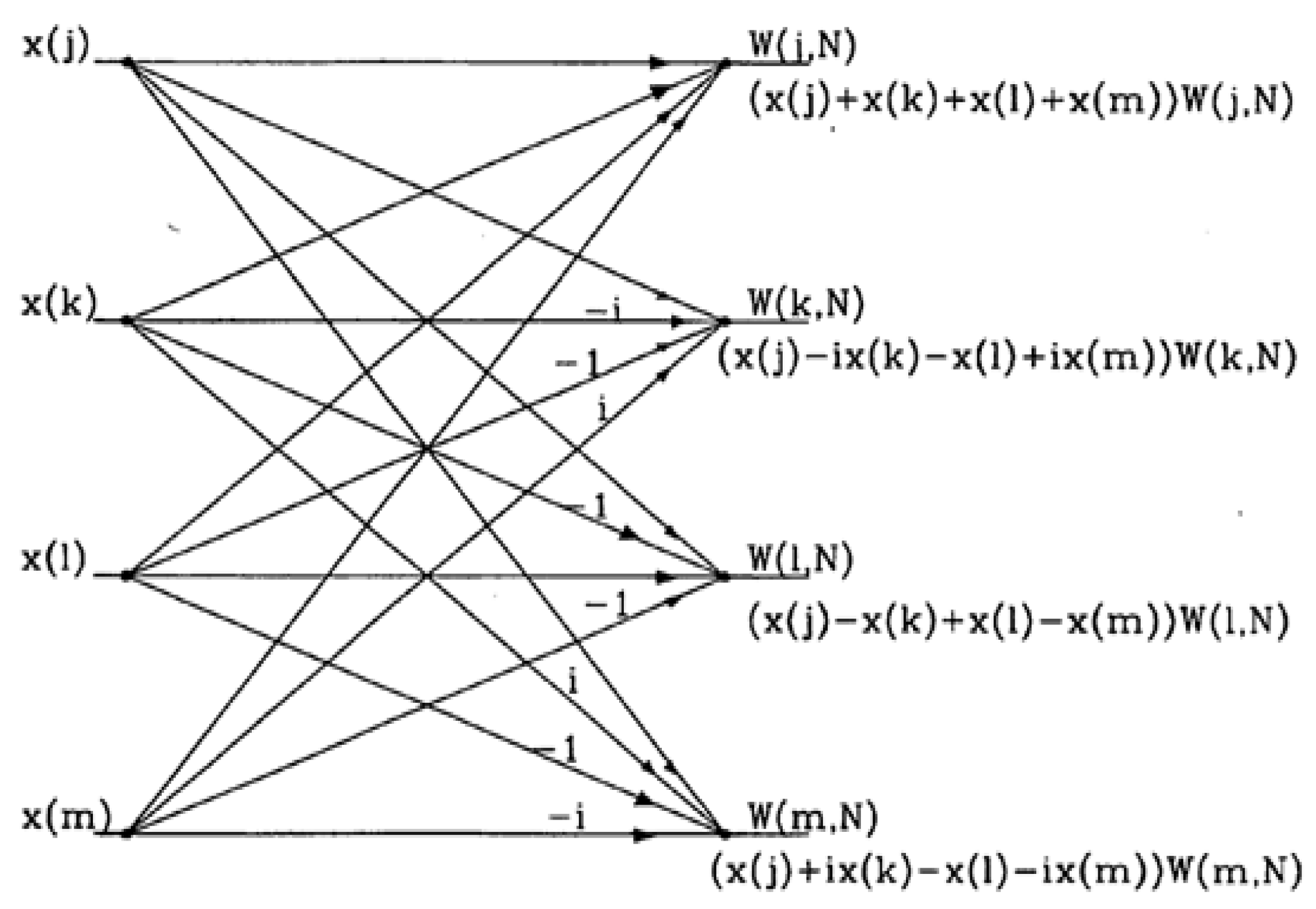
After the division of N-point DFT, it can be computed as the sum of the outputs of four N/4-point DFTs, and these sub-sequences are interconnected with so-called twiddle factors W^lk _N = e^{−(j2lᴫk/N)}, l = 0, 1, 2, 3, as shown in (4).

$$\begin{gathered} X\left(k\right)=\sum _{n=0}^{N-1}x\left(n\right)W_N^{nk} \\ =\sum _{n=0}^{\frac{N}{4}-1}x\left(n\right)W_N^{nk}+\sum _{n=\frac{N}{4}}^{\frac{N}{2}-1}x(n)W_N^{nk}+\sum _{n=\frac{N}{2}}^{\frac{3N}{4}-1}x\left(n\right)W_N^{nk}+\sum _{n=\frac{3N}{4}-1}^{N-1}x(n)W_N^{nk} \end{gathered}$$

(4)

Thus,

$$X\left(k\right)=\sum _{n=0}^{\frac{N}{4}-1}x\left(n\right)W_N^{nk}+W_N^{\frac{Nk}{4}}\sum _{n=\frac{N}{4}}^{\frac{N}{2}-1}x\left(n+\frac{N}{4}\right)W_N^{nk}+W_N^{\frac{Nk}{2}}\sum _{n=\frac{N}{2}}^{\frac{3N}{4}-1}x\left(n+\frac{N}{2}\right)W_N^{nk}+W_N^{\frac{3Nk}{4}}\sum _{n=\frac{3N}{4}-1}^{N-1}x\left(n\right)W_N^{nk}$$

(5)

Final representation of X(k) is,

$$X\left(k\right)=\sum _{n=0}^{\frac{N}{4}-1}\left[x\left(n\right)+{\left(-j\right)}^{k}x\left(n+\frac{N}{4}\right)+{\left(-1\right)}^{k}x\left(n+\frac{N}{2}\right)+{\left(j\right)}^{k}x(n+\frac{3N}{4})\right]W_N^{nk}$$

(6)

According to Equations (4)–(6), the process is called decimation in time because the samples of time are arranged into groups. The basic operation of the R4 butterfly is shown in Figure 1 [17]. The decimation-in-time process consolidates the inputs at each stage of decomposition, resulting in “input order that is bit-reversed” at the end. This set-up allows for the intermediate outputs to be stored in the same memory regions as the inputs (in-place algorithm). The radix-4 FFT’s slight reorganization allows the inputs to be redirected from digit to bit [18], as shown in

Table 2. Numbering according to base-4 for bit reverse.

Normal Sequence Order	Normal Sequence Bit Order	Reversed Bit Order	Reversed Sequence Number
0	000	000	0
1	001	100	16
2	002	200	32
3	003	300	48
4	010	010	4
5	011	110	20
14	032	230	44

.

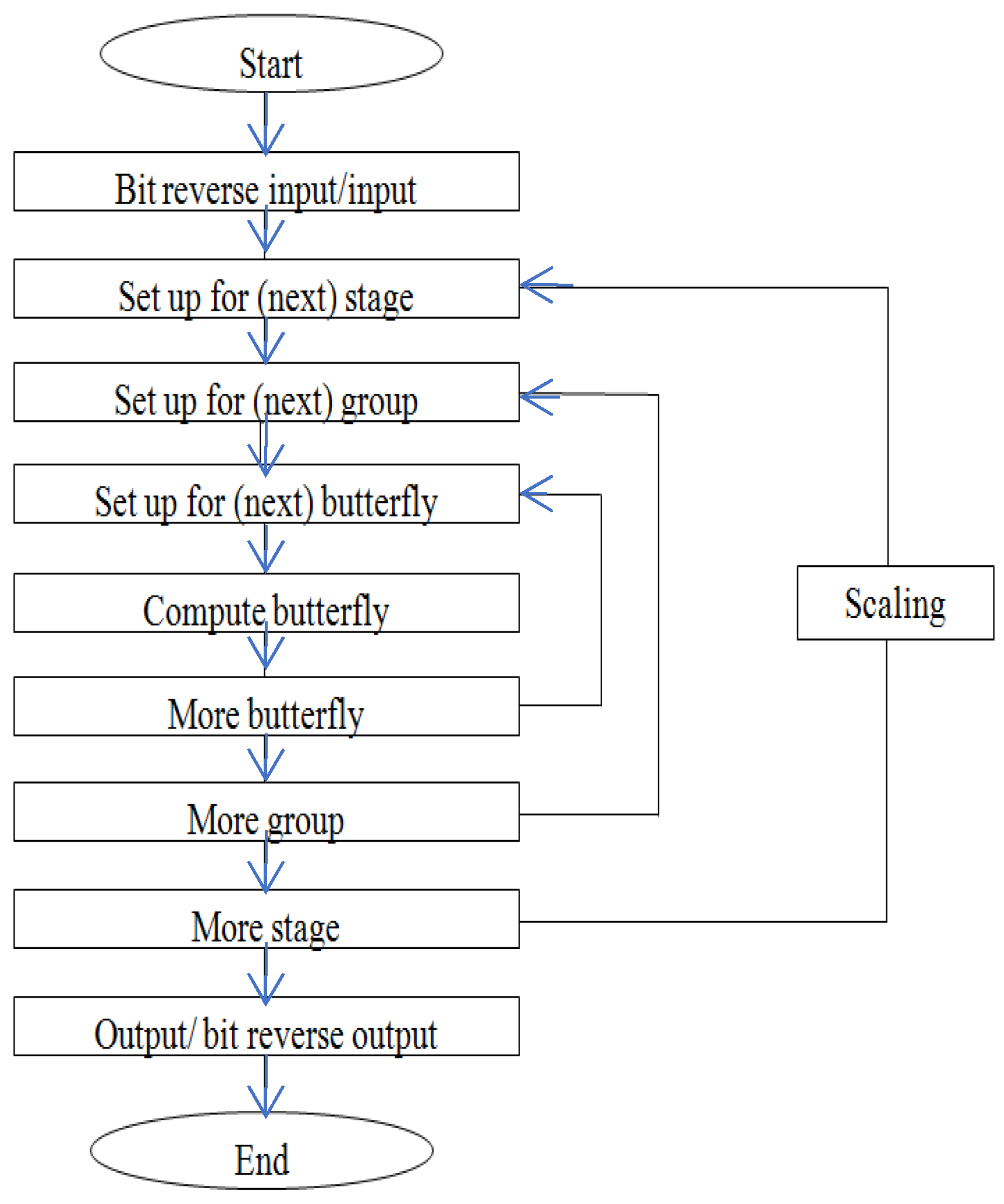
Figure 2 depicts the computation of the radix-4 project’s flow chart. The input sequence might be in bit reversal order or normal order. The updated sequence can be operated on after being arranged. Each stage has a group of butterflies, and each butterfly group is made up of other butterflies. After that, the butterfly (radix-4) algorithm is used. For each further stage or group, the operation repeats until all butterflies in a group and stages have been completed by scaling with the required twiddle factor. Here, the radix-4 operation is completed with the output in either a normal or bit-reversed order depending on the input sequence [15,16,17,18] and radix-4 operations are completed.

The radix-2 adds twiddle integer factors at 0° and 180° angles, whereas radi-x4 adds twiddle integer factors at 0°, 90°, 180° and 270° angles, all while accounting for the computational cost of multiplication. There is no need to multiply the sine and cosine counterparts of the above-mentioned angles within a unit circle. The radix-8 is not preferred because of its factors of fractional twiddle 2 at 45°, 135°, 225° and 315° in a unit circle, despite the fact that the number of radixes minimizes the number of computation steps [19,20].

2. Development of a Lossless Medical Image Compression Using FFT Algorithm

Medical image compression using FFT is developed as shown in the flow chart given in Figure 3. Load/read any medical input image and convert it into a 2D array of a double image. Compress the loaded image with different tolerance values. While compressing the image, it takes as inputs the original image X and the drop tolerance parameter and outputs a compressed image Y. It also returns the drop ratio given in Equation (7), which is defined to be as the ratio of “Total number of nonzero Fourier coefficients dropped to the Total number of initially nonzero Fourier coefficients”.

For every drop count for a compressed image, apply FFT to each sub block.

Drop ratio = (Total number of nonzero Fourier coefficients dropped/Total number of initially nonzero Fourier coefficients)

(7)

3. Results and Discussion

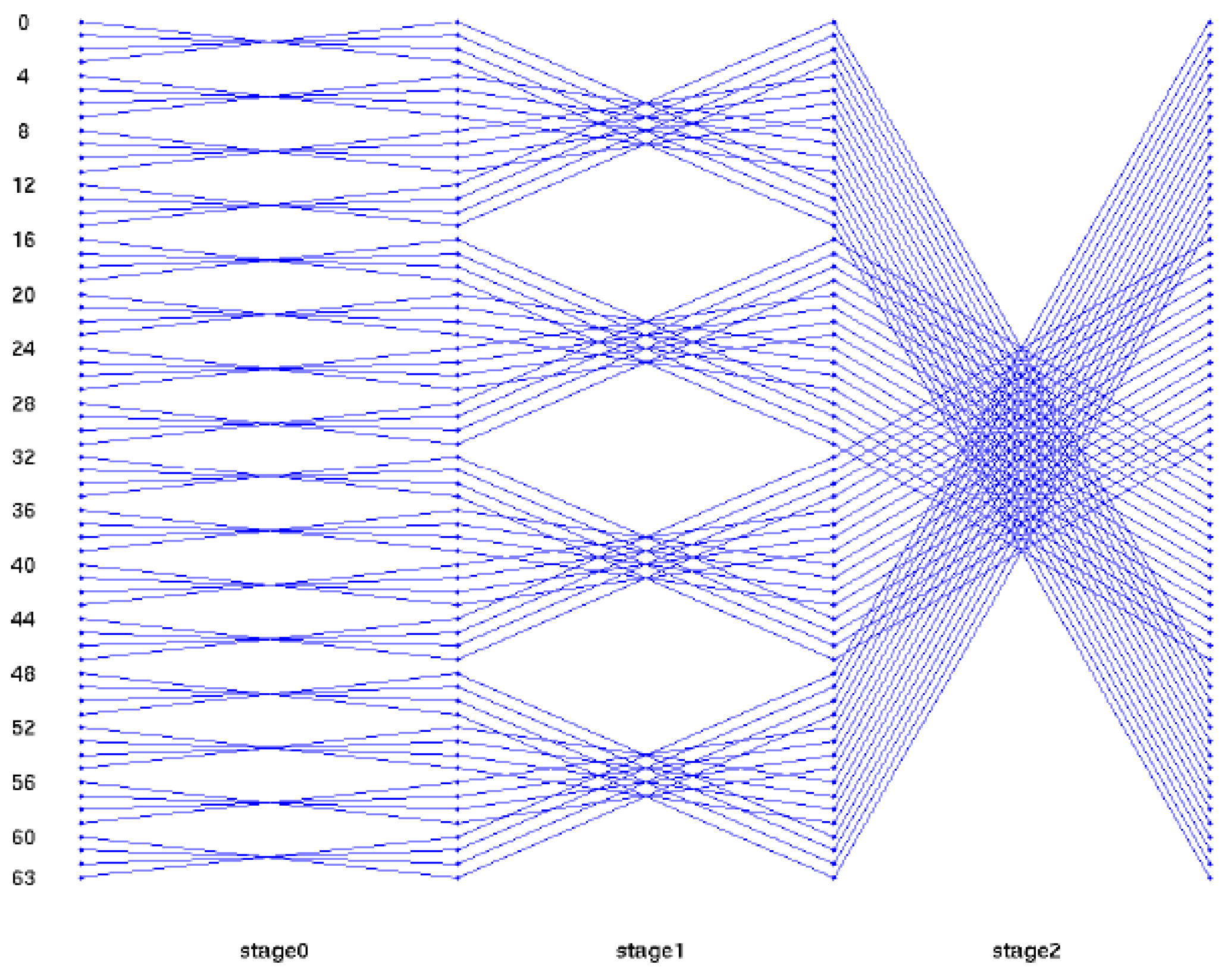
A 64-Point DFT using the radix-4 DIT-FFT algorithm has three stages. In the first stage, 16 blocks are present, and each block consists of only one butterfly. In the first stage, the inputs are applied in a bit-reversal order to save memory space. In the second stage, there are four blocks, and each block consists of four butterflies as a set. Totally, four sets are present. In the third stage and in the final stage, only one block is present in that 16 butterflies are present as one set, and the output is finally obtained from the final stage, which is in a normal order. 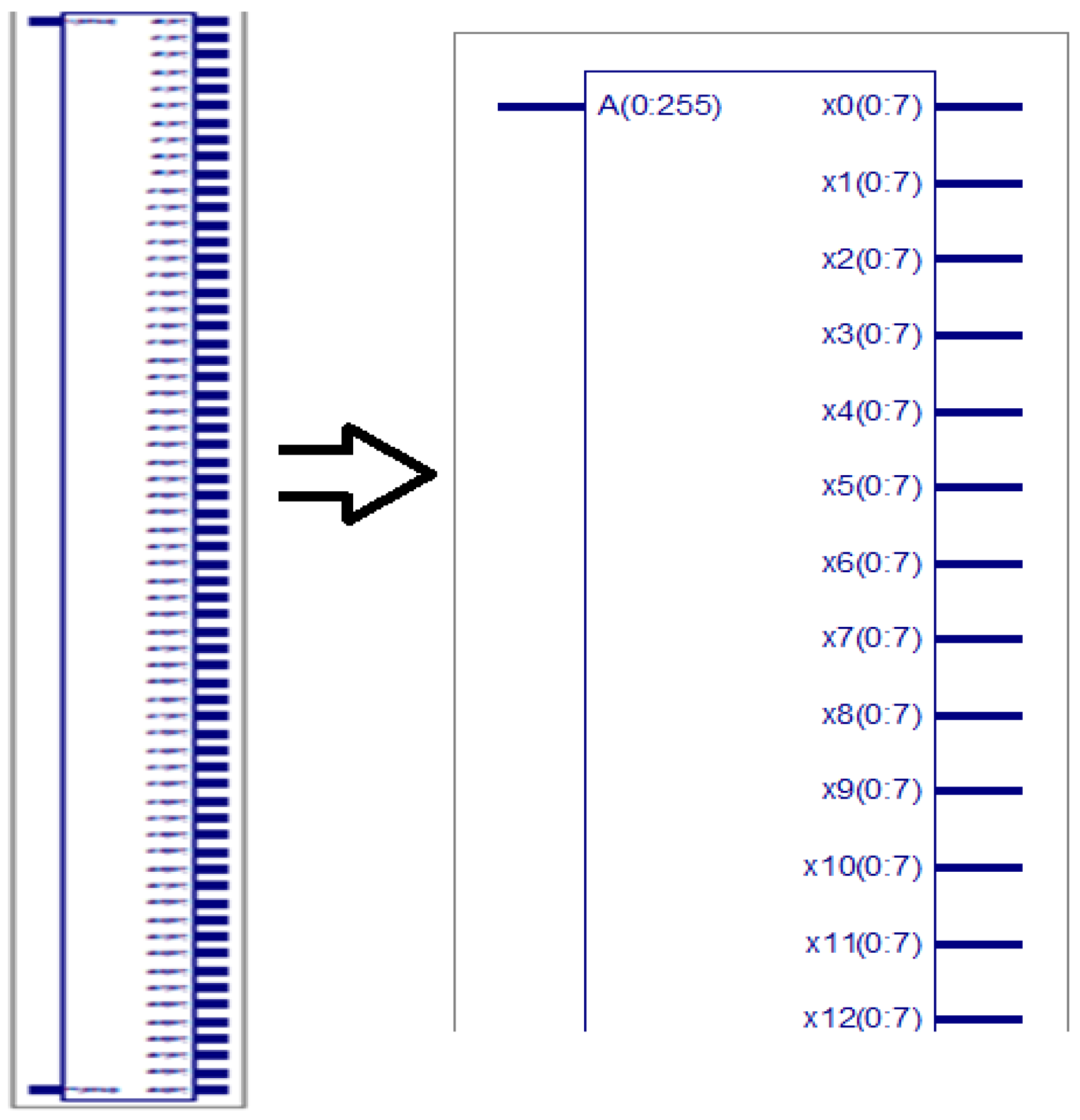A structural view of the 64-point radix-4 DIT-FFT is shown in Figure 4. The Register-Transfer Level (RTL) view of the proposed algorithm consists of data splitting of 256 bits into 4 64 bits, and each section of 64 bits is further divided into 16 4-bit points and separated into even and odd sequences. All are communicated with a communicator called Commutator.

The target XC3S500E-5FGG320C Xilinx FPGA, Guntur, India is used for the execution. The device contains the 9312 LUTs and 4656 slices for functionality of the input sequence. Slices used for the related logic are 3286 and 3286 for the unrelated logic. The device contains 9312 four-input LUTs and works under a speed grade of ‘-5’.

Generally, the 64-point radix-4 DIT-FFT butterfly unit (butterfly 16) consists of butterflies, sets of butterflies and stages (Figure 4). The entire code was developed in a structure made using HDL language. The internal modules were designed based on the behavioral model or dataflow model. The different internal modules are: splitting the entire sequence into equal parts to save memory, 4-bit butterfly unit, odd and even parts, butter for 8-point and 4-point and Commutator for connecting all the stages and sub modules. All these modules are called sub modules in the top butter. The RTL view and simulation result of the 64-point radix-4 DIT-FFT are shown in Figure 5.

3.1. Data Split of 64 Points

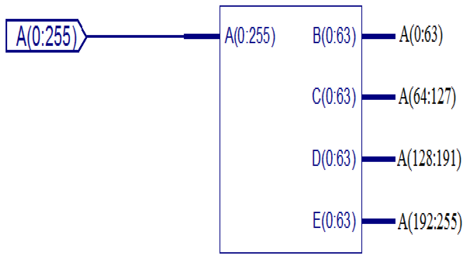
The entire 64-point radix-4 DIT-FFT can be split into four equal parts. Each of the 16 points and each point are the combination of 4 bits; totally, 64 bits are in each equal part. A is an input sequence of 256 bits (0 to 255), divided into four equal parts of each 16 point 64 bit (0 to 63, 64 to 127, 128 to 191, 192 to 255). The RTL view of data split 64 points into four equal 16 points, and the simulation results are shown in Figure 6, Figure 7 and Figure 8, respectively.

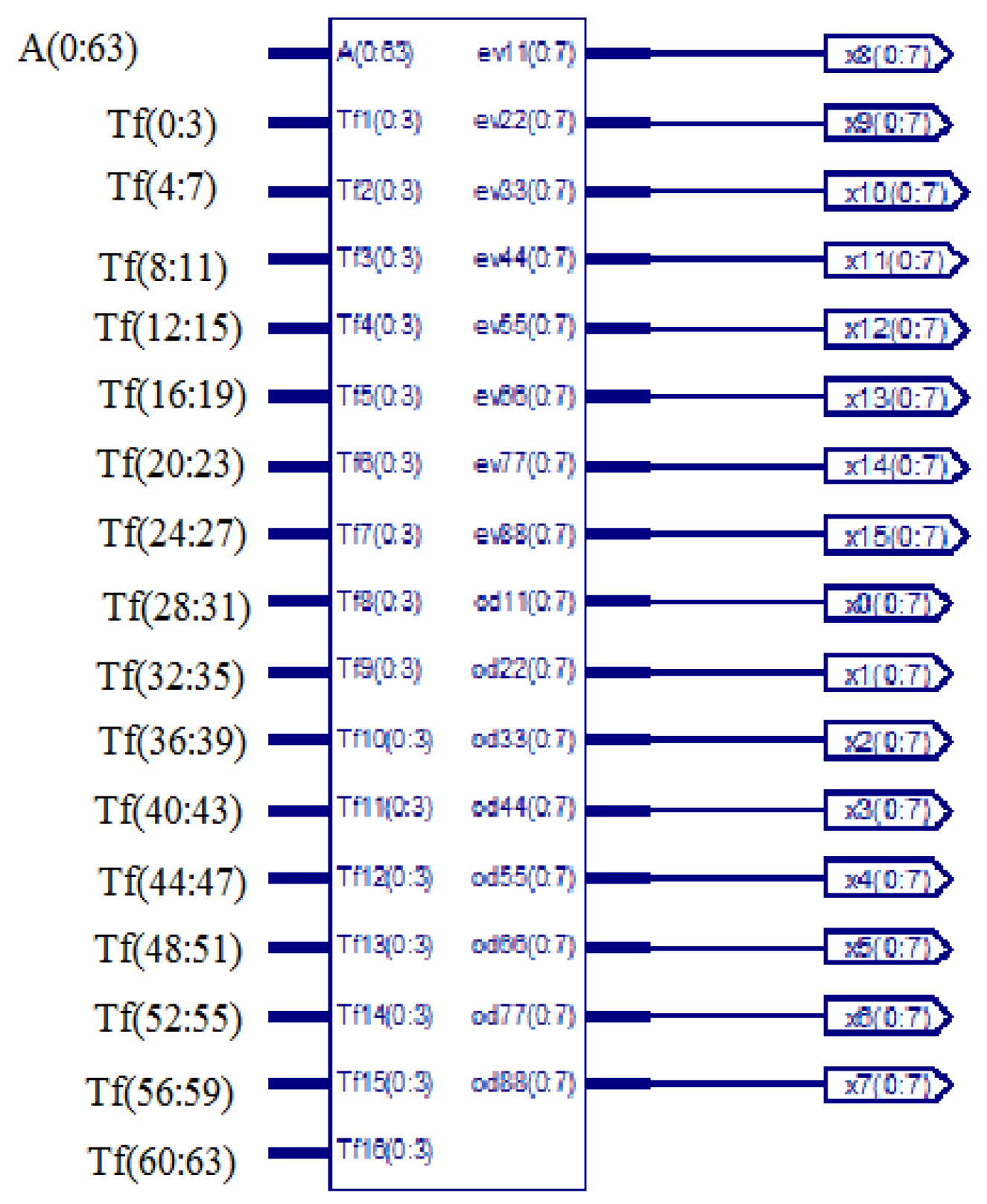
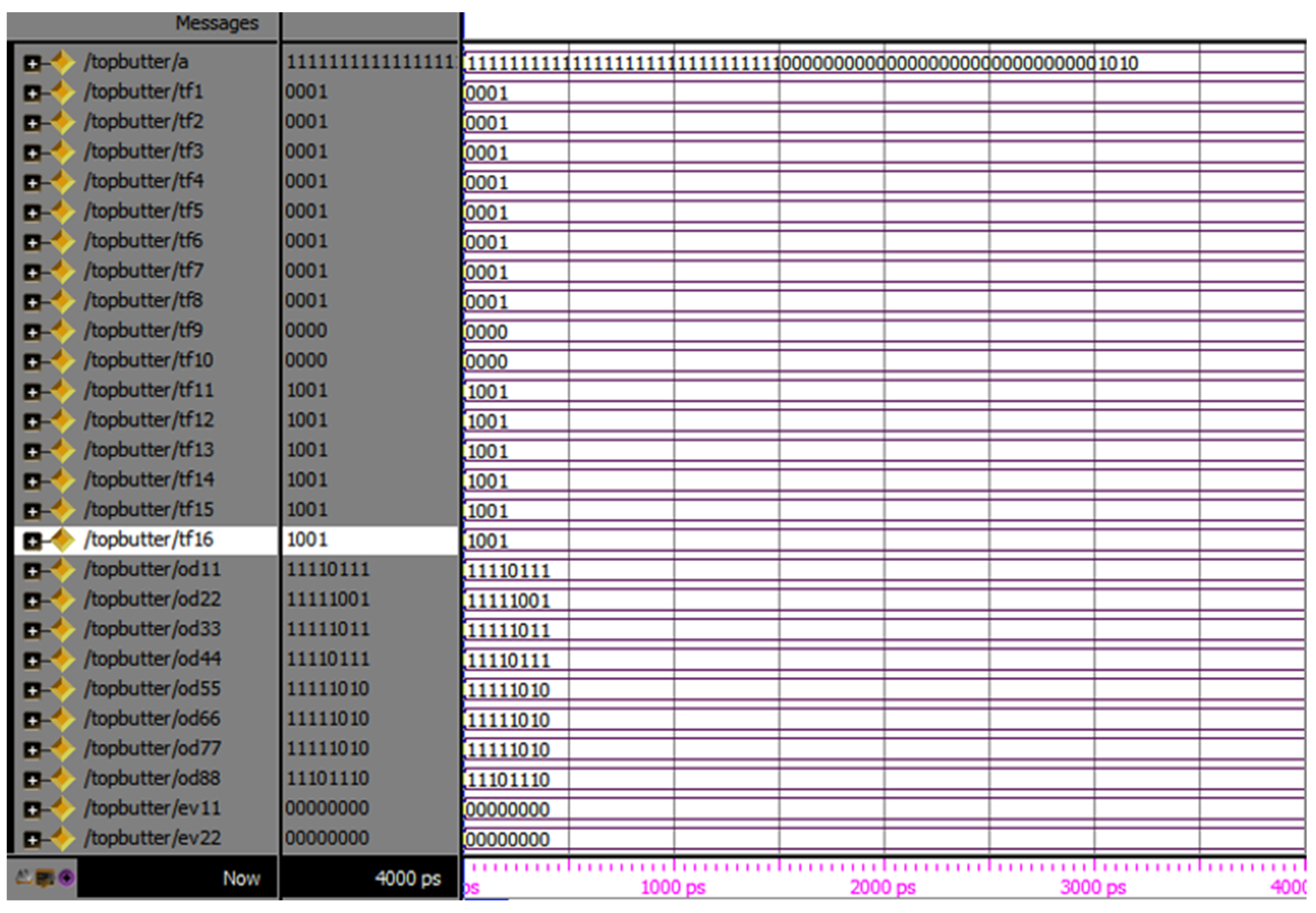
3.1.1. Top Butter

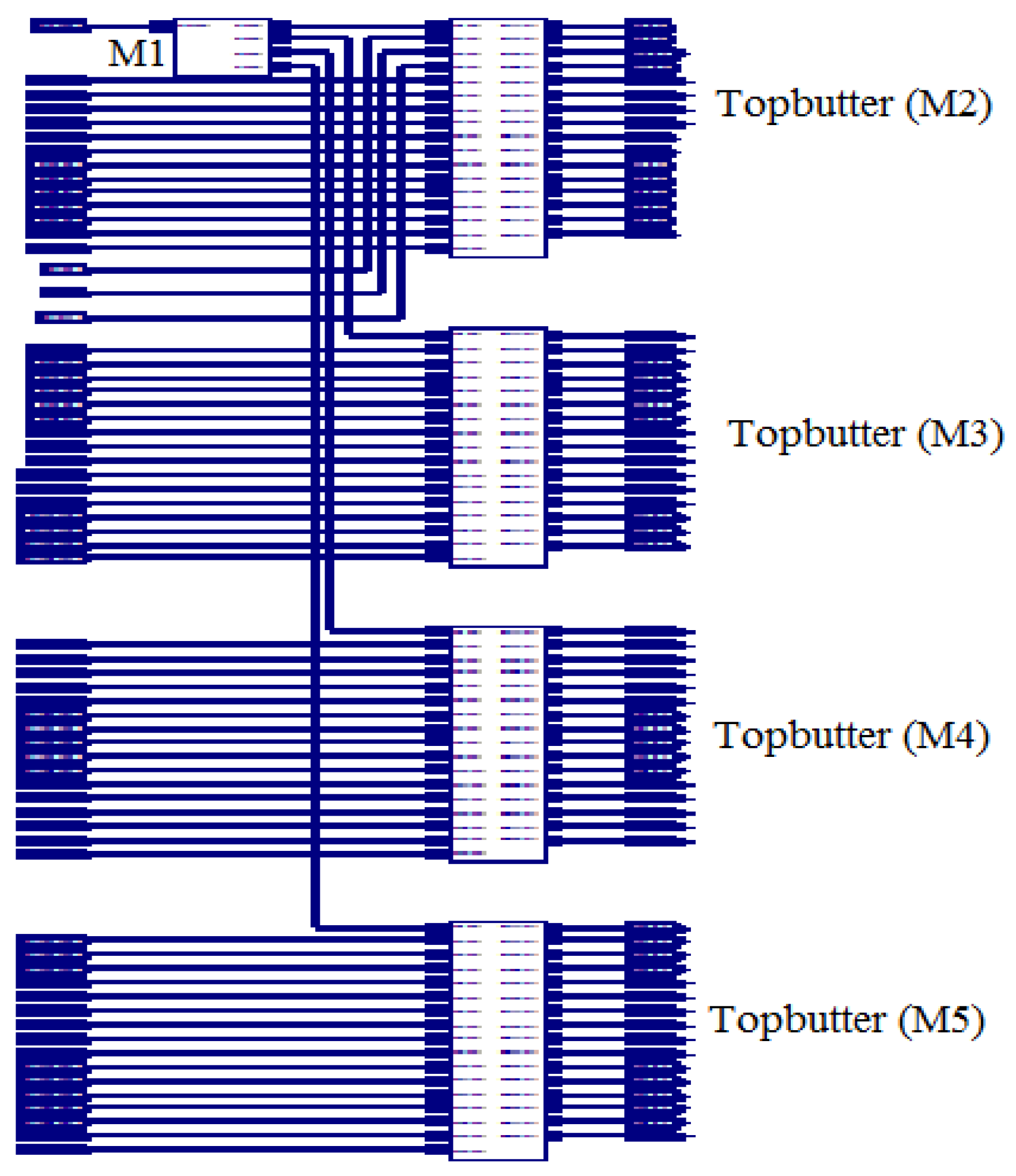
Top butter is the divided part of the entire sequence. This has a 16-point, 64-bit input and 64 twiddle, totally 128-bit output, in which 64 bits are even and the remaining bits are odd. Top butter contains the Commutator, even and odd parts. For the entire sequence, the total 4-top butters (M2, M3, M4 and M5) are present. The RTL view of the top butter (M2), and the simulation results are shown in Figure 9 and Figure 10, respectively:

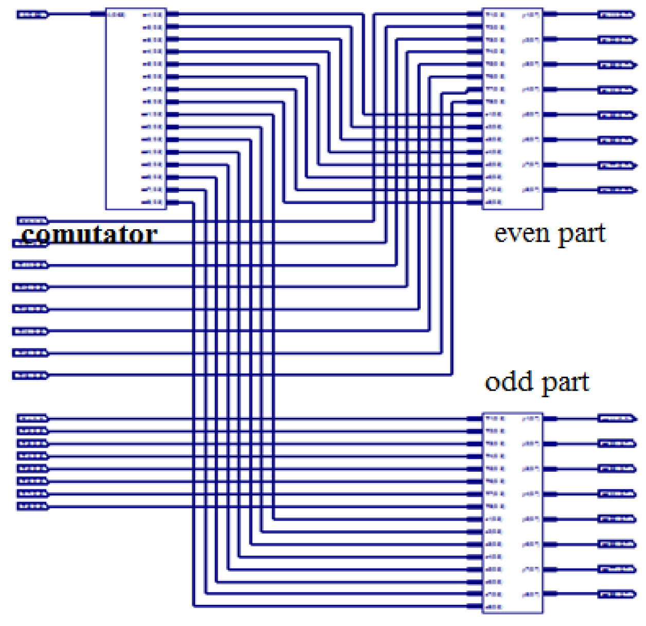
3.1.2. Internal Structure of Top Butter

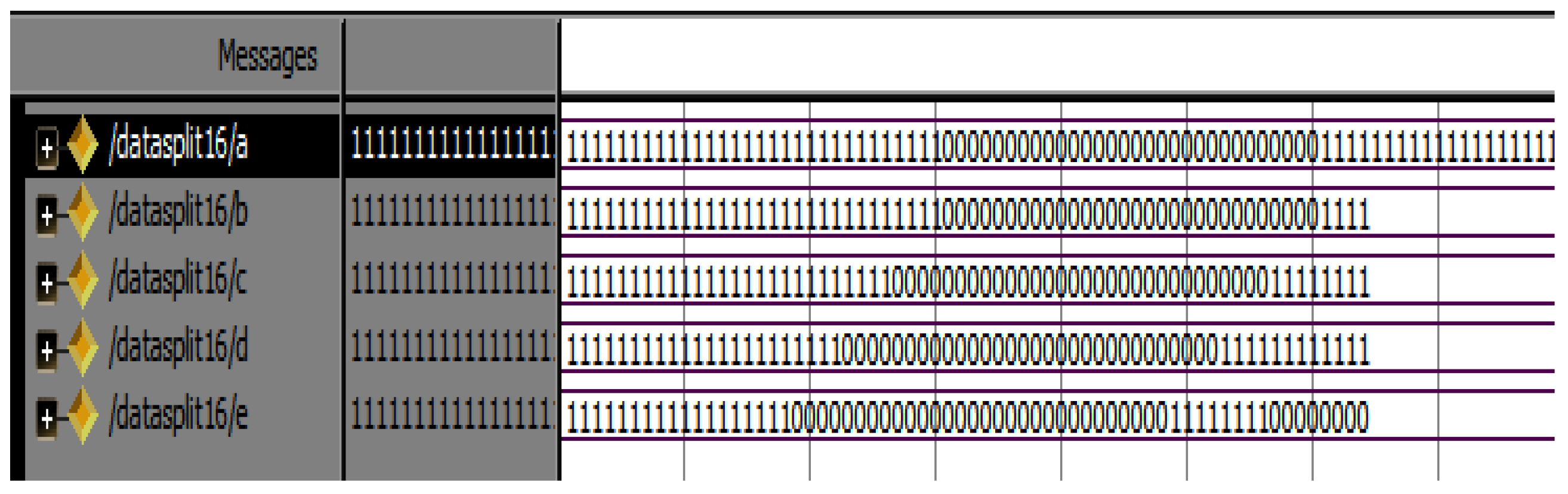
The equally divided 16-point (64-bit) sequence again undergoes further division to increase the speed of execution. The 64-bit (0 to 63) sequence divides as A (0 to 3), A (4 to 7) and so on to A (59 to 63), and 16 points are divided into the remaining four equal parts. The simulation results of data split of 16 points are shown in Figure 11 and Figure 12 and RTL view of this unit having Commutator (Figure 13 and Figure 14), even and odd parts respectively:

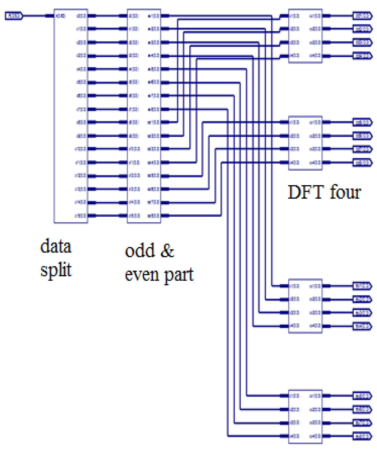
3.1.3. Commutator

As commutator is used to communicate, it consist of data splitter, odd and even parts, DFT four bit odd and even parts separately as shown in Figure 13 and its simulated results is shown in Figure 14.

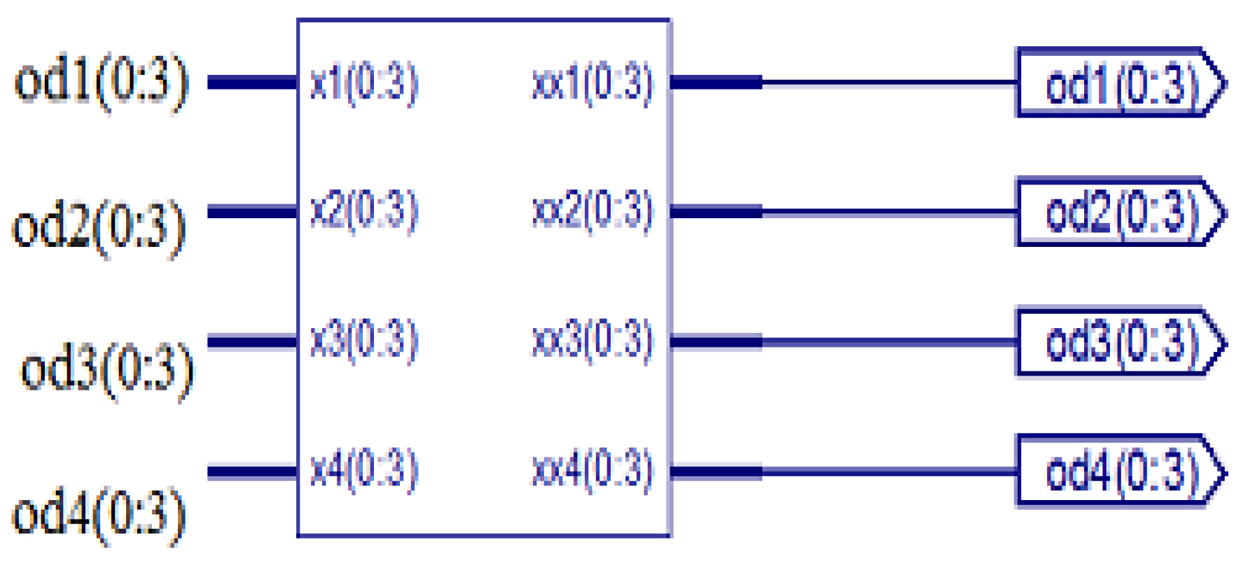
3.1.4. DFT Four

DFT four is the basic unit in the radix-4 structure, because it transfers the input value to output. Each stage has this unit, and four inputs and four outputs are present in this unit. The RTL view and simulation results of DFT four are shown in Figure 15 and Figure 16, respectively.

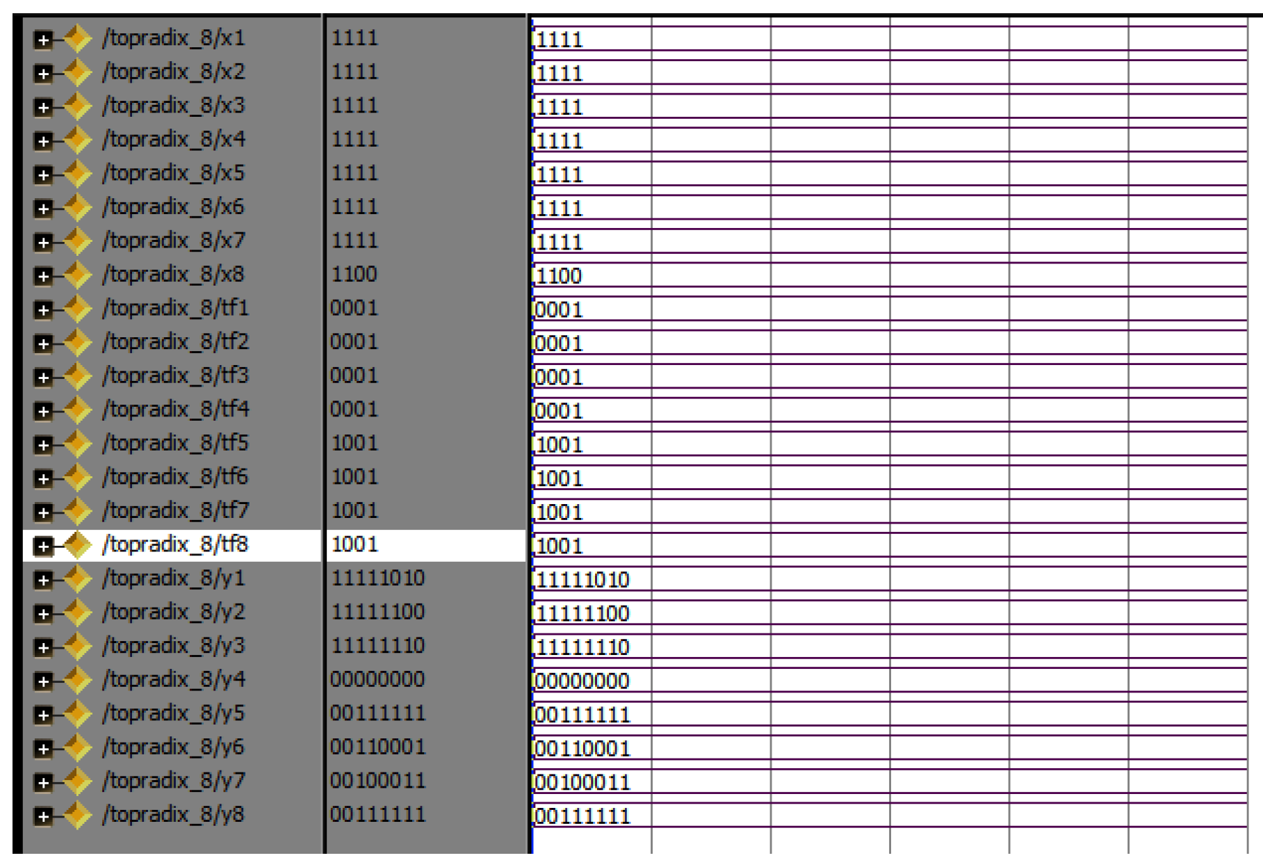
3.1.5. Butter R8

Butter R8 is the internal unit in the butterfly diagram. It is the combination of both even and odd parts. Each even and odd part is the combination of two butter R4 blocks, so there are a total of two R4 blocks for each butter R8 block. This butter R8 block exists from the 16-point block means division of 16 points into smaller parts for easy execution. The RTL view and simulation results of butter R8 are shown in Figure 17 and Figure 18, respectively.

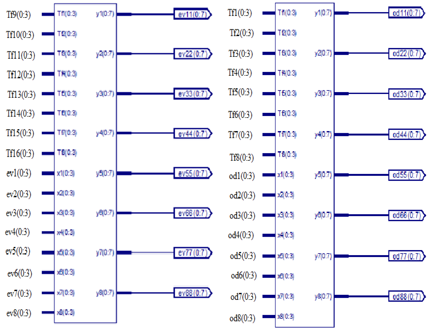
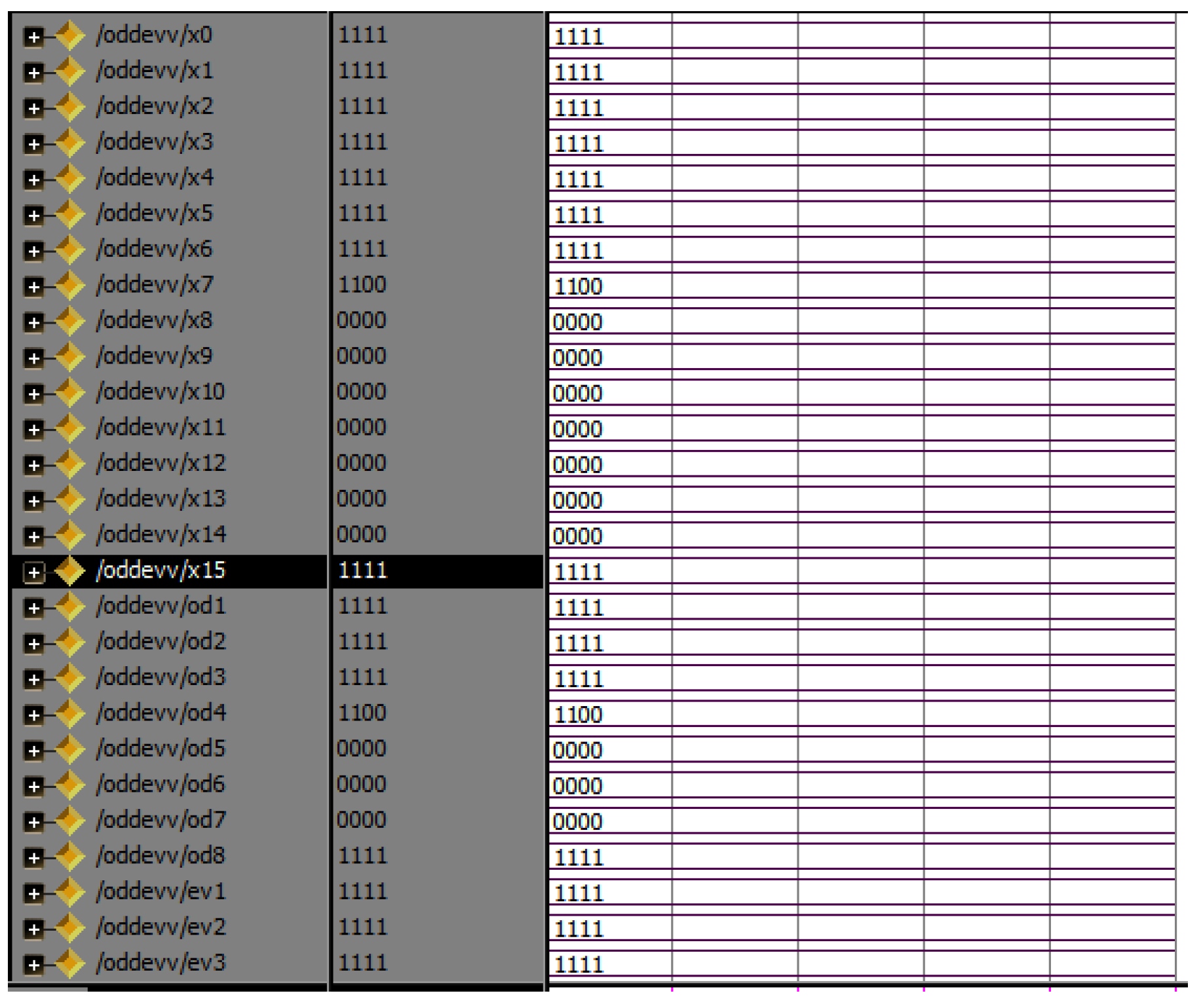
3.1.6. Even and Odd Parts

Even and odd parts are the two different functions in the entire butterfly unit. The combination of even- and odd-part units is present in all modules (M2, M3, M4 and M5). In four modules, four even- and odd-part combinations are present. In the different parts, the divided sequence can be ordered into even and odd parts/places to save memory requirements. The even and odd parts have two instances internally to make the execution easier. The simulation results are shown in Figure 19.

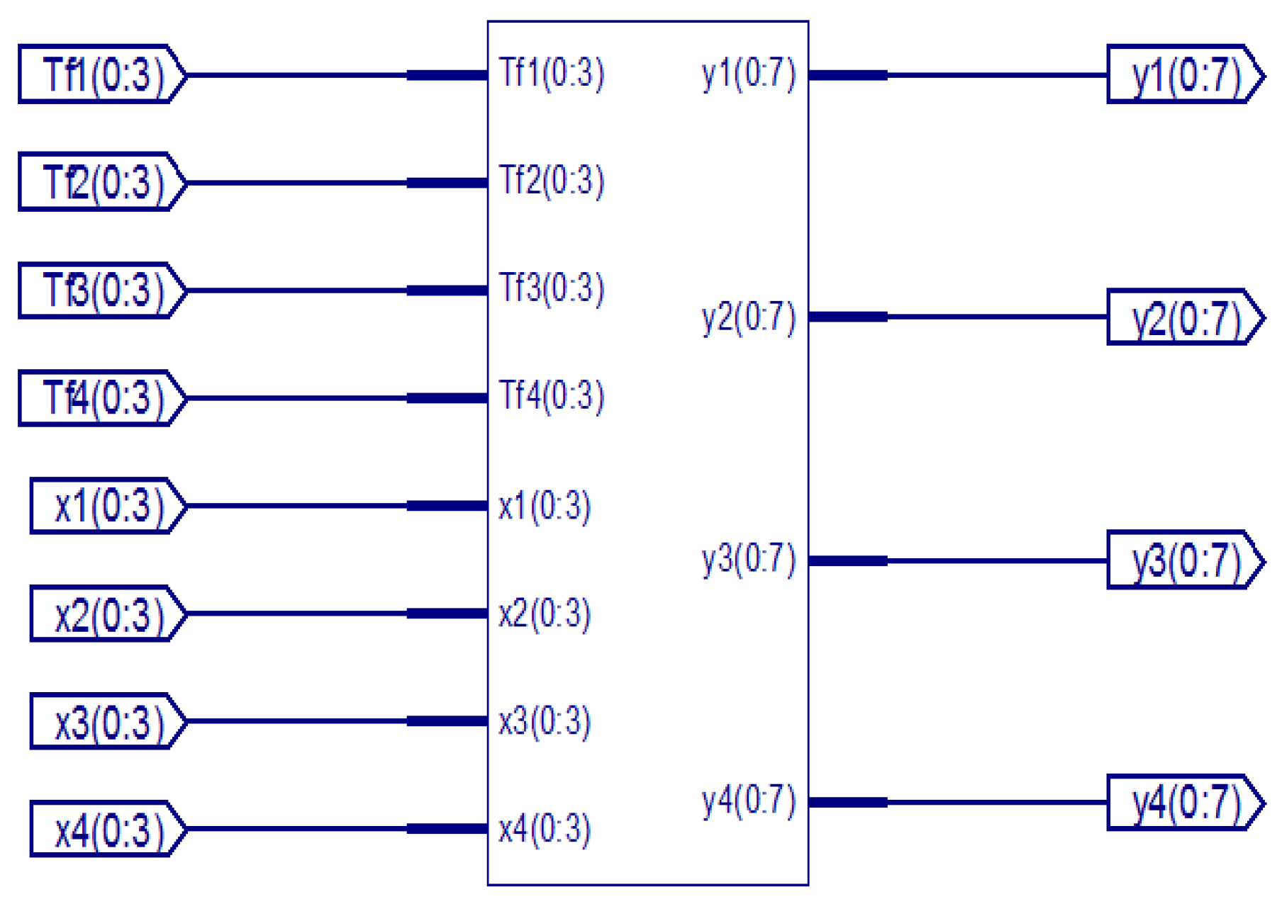
3.1.7. Butter R4

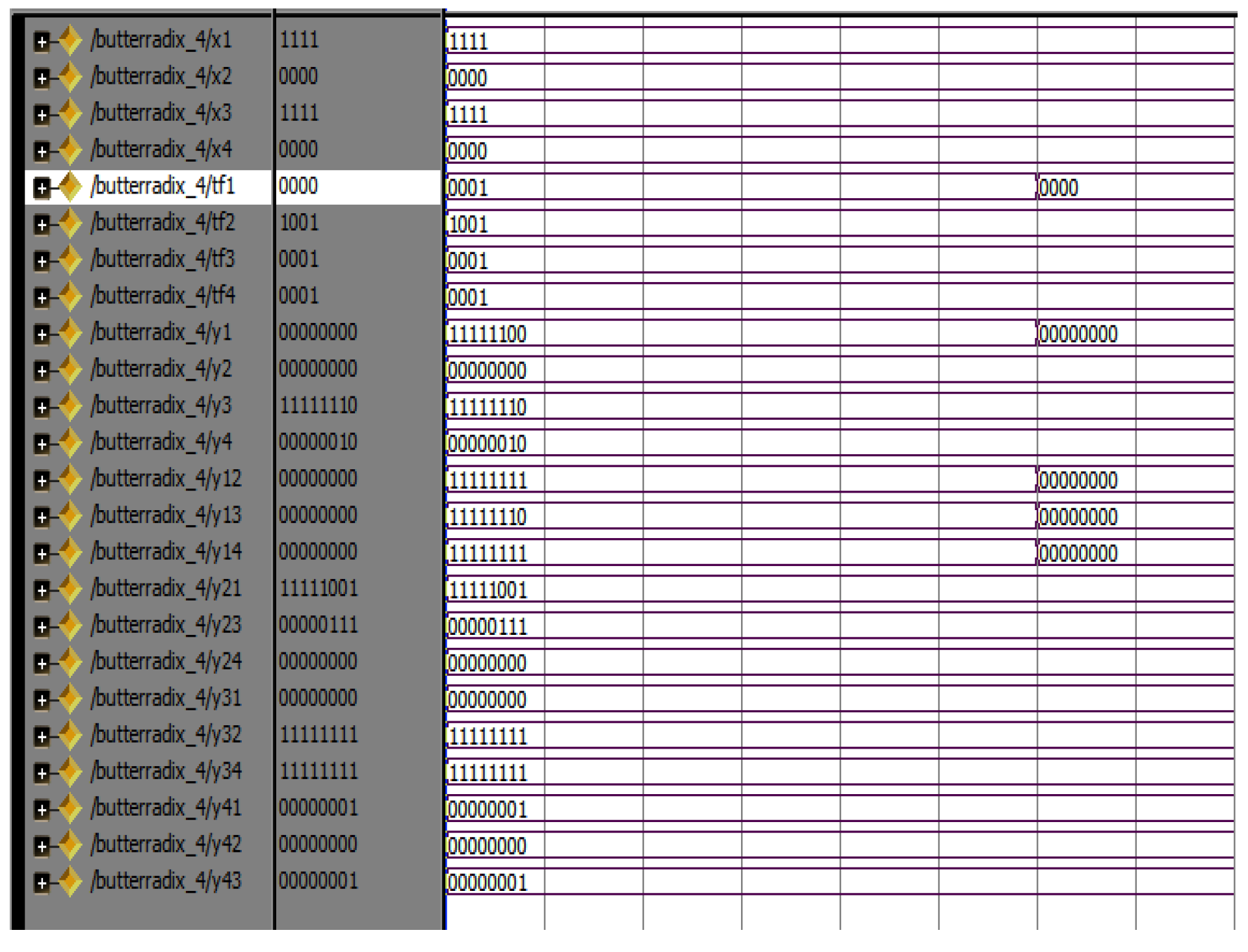
Butter R4 is the basic unit in this structure because it represents the radix-4 function. Each stage has this unit, either as a single unit or as a set/group. In this unit, four inputs and four outputs are present, as shown in the Figure 14. Each input is multiplied with the twiddle factor and gives the output, implying that for the 256-bit input, there are 256 twiddle factors present. The RTL view and simulation results of butter R4 are shown in Figure 20 and Figure 21, respectively.

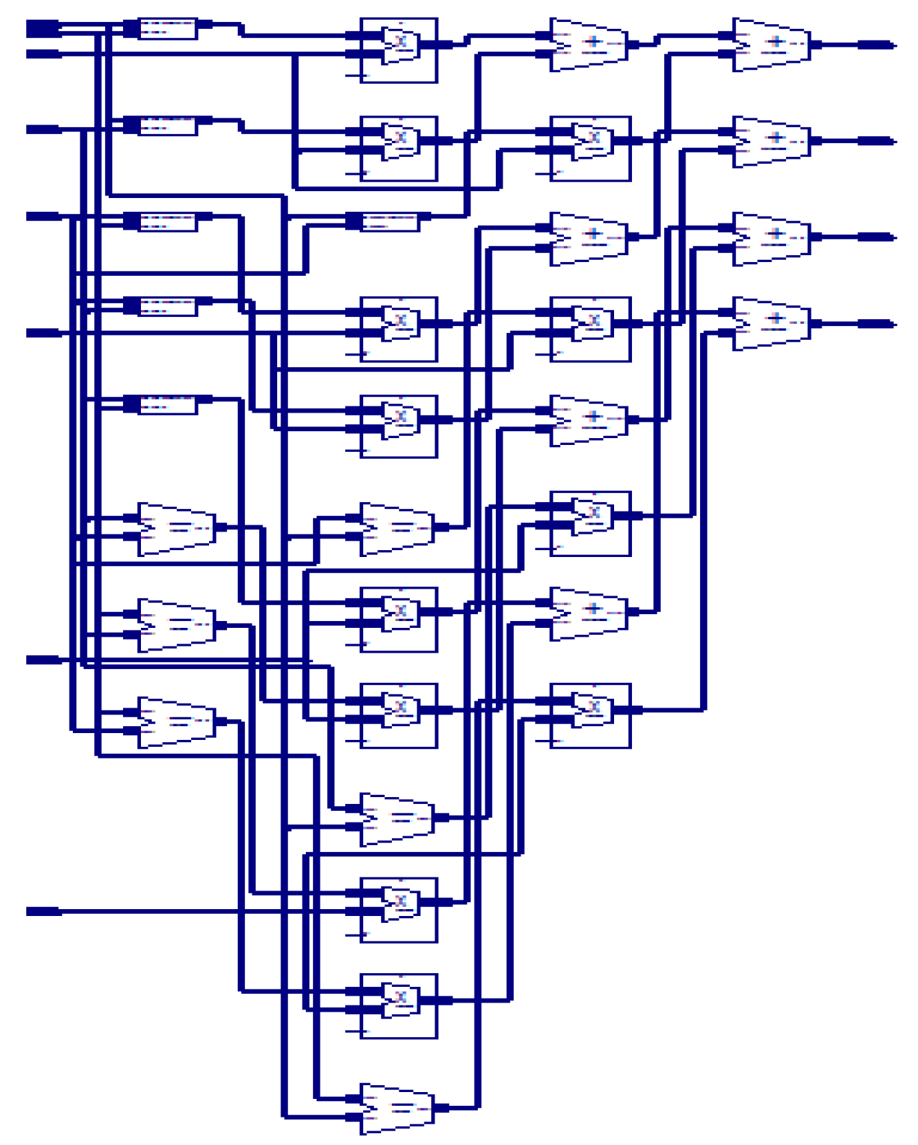
3.1.8. Internal Structure of Butter R4

The internal structure of butter R4 consists of different units. These units are responsible for the entire functionality of the butterfly unit. The different units are adders, subtractors and multipliers, and these units are called basic building blocks for butter R4. The RTL view is shown in Figure 22.

3.2. Simulation Results of Radix-4 Algorithm

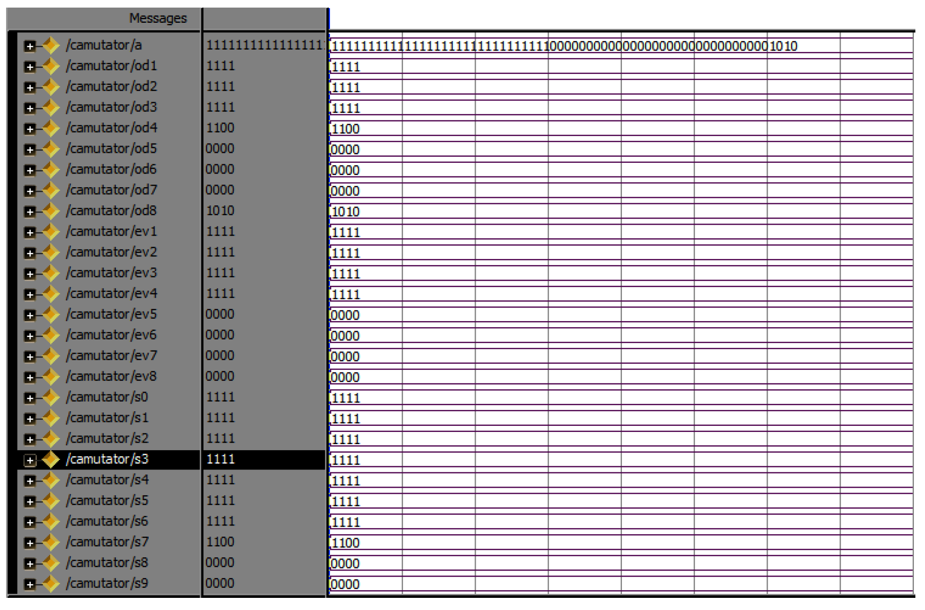
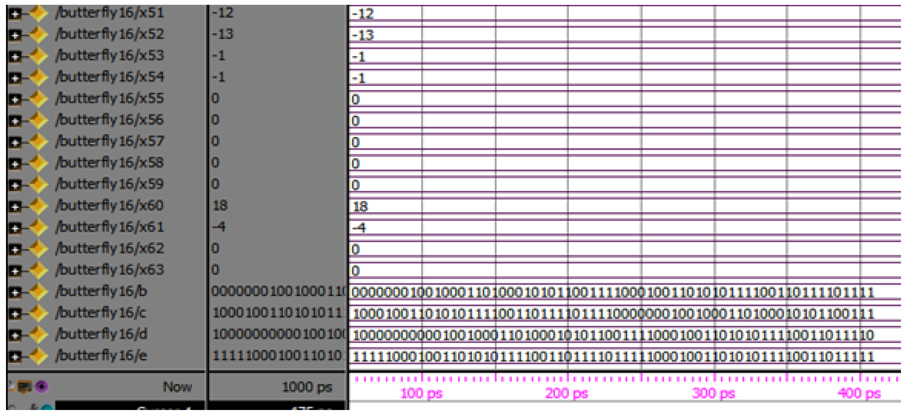
Figure 23 shows the simulation results of the 64-point radix-4 DITFFT butterfly block. The A of each of the 4 bits, totally, is 256 bits. W of 256 points represents the inputs and twiddle factors. The X is an output of 64 points for each point of 8 bits, since the even and odd part results, totally, in 512 points, all in binary formats.

3.3. Timing Report

The timing report is generated under a speed grade of -5. This report includes all the input and output cells and their fan out. Each gate delay and net delay is also considered, and the summation of gate delay gives the timing delay of the project as 19 ns. The comparison between the performance of the radix-2 and radix-4 algorithms based on different aspects, such as number of slices used, LUTS, bonded IOBs, flip flops and global clocks, for their operations.

From

Table 3. Performance comparison between the radix-2 and radix-4 algorithms.

Device Utilization	Radix-2			Radix-4
	Used	Available	Utilization (%)	Used	Available	Utilization (%)
Slices	2388	4656	51	3332	4656	71
4 input LUTs	4282	9312	45	5936	9312	63
IOBs	135	232	58	1024	232	441
Delay	75.050 ns			18.963 ns
Memory	0.206720 GB			0.228 GB
Power	56.78 mW			12.68 mW

, it is observed that the minimum delay for the functioning of inputs and outputs for radix-4 is significantly less when compared with radix-2, and memory usage is almost the same as radix-2 and even radix-4 using a greater number of inputs. We observed that 75% of the computations were saved in radix-4, even though the device utilization was higher.

Table 4. Performance comparison among the proposed FFT with existing works.

Parameter	This Work	[2]	[8]	[10]	[14]
FFT Size	64-4	32-8	64-4	16-4	16-4
Delay (ns)	18.96	419	8.10	2.2	2.67
Power (mW)	12.68	739.5	33.5	3.5	4

shows the performance comparison of size, delay and power of previous existing methods.

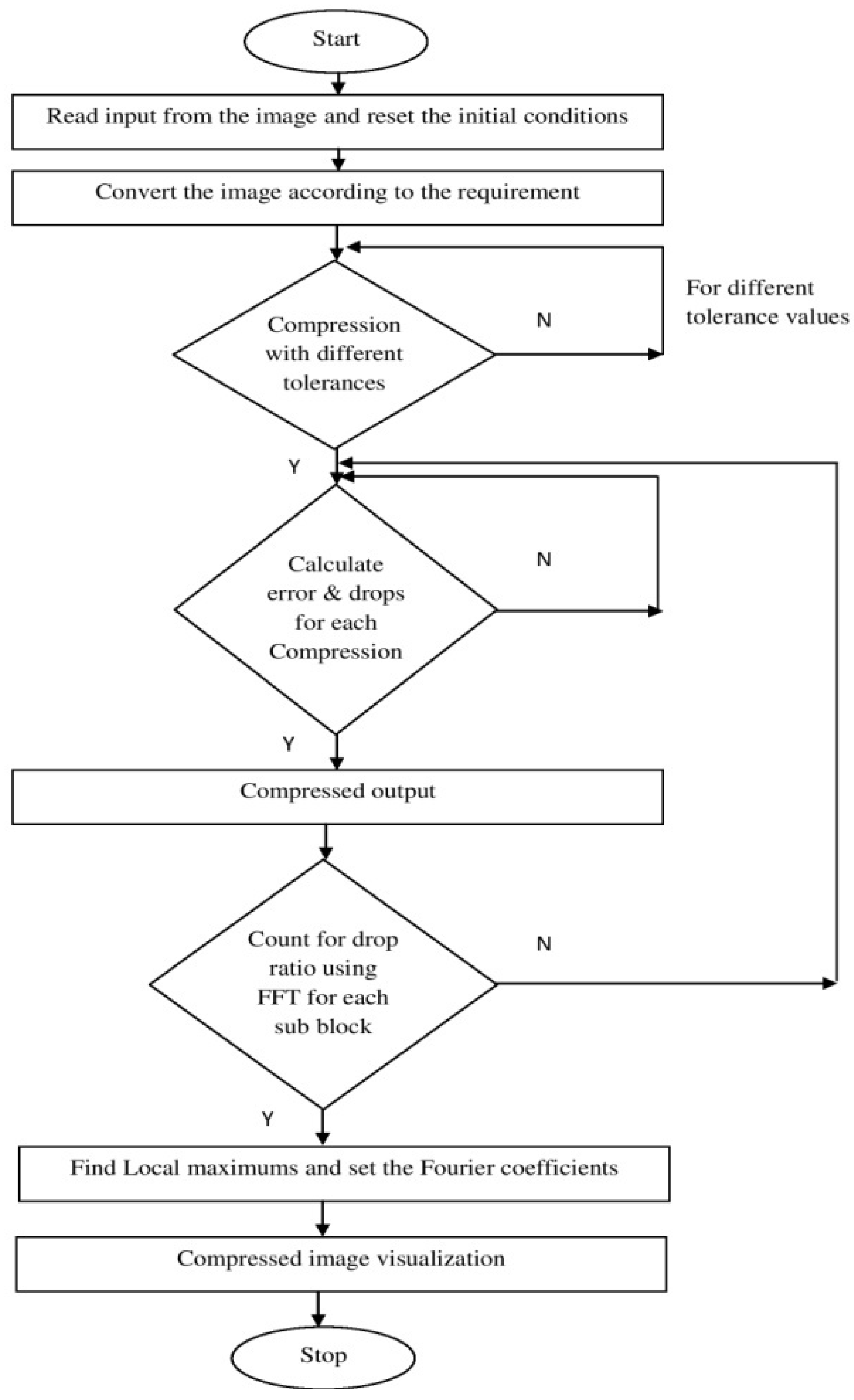
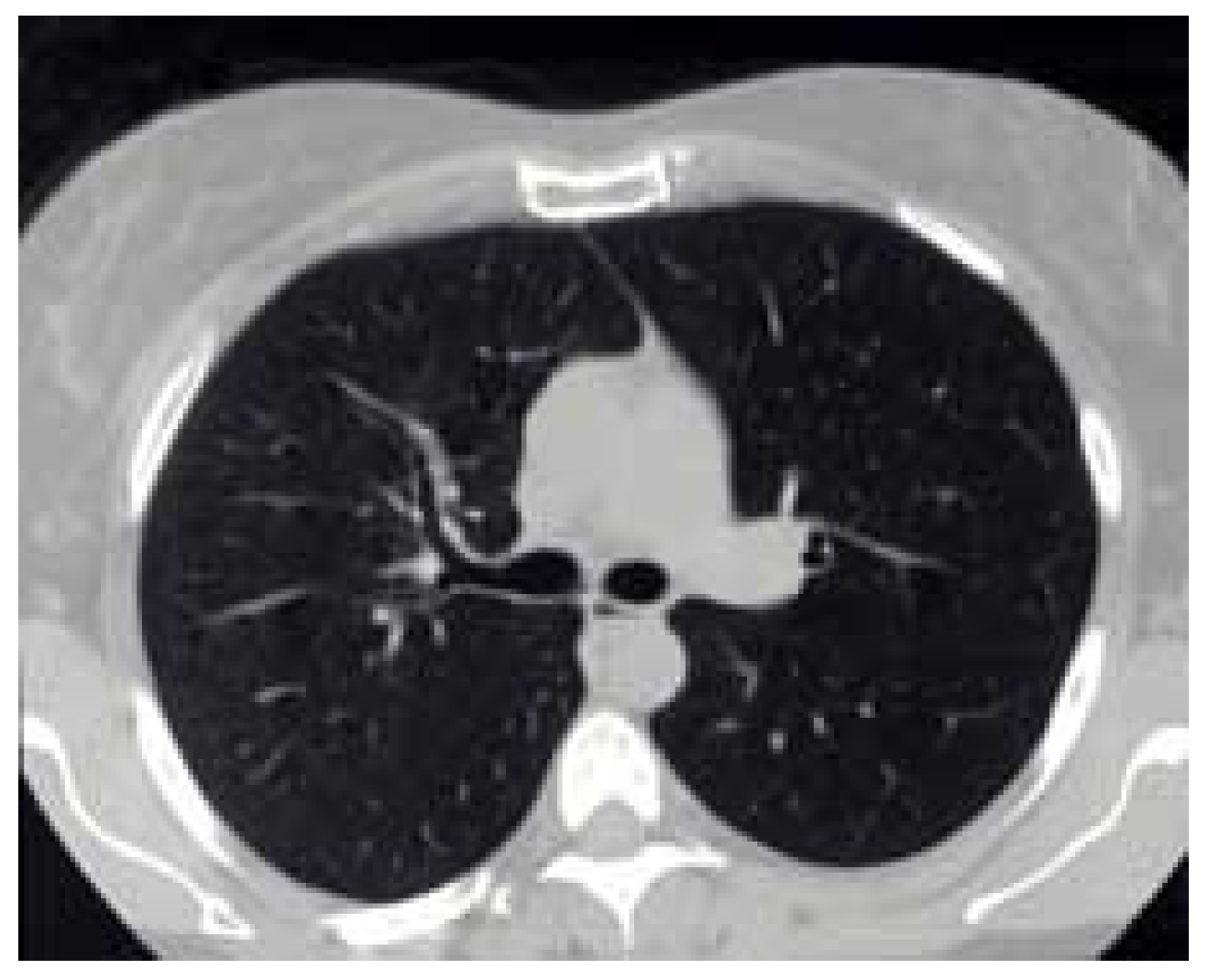
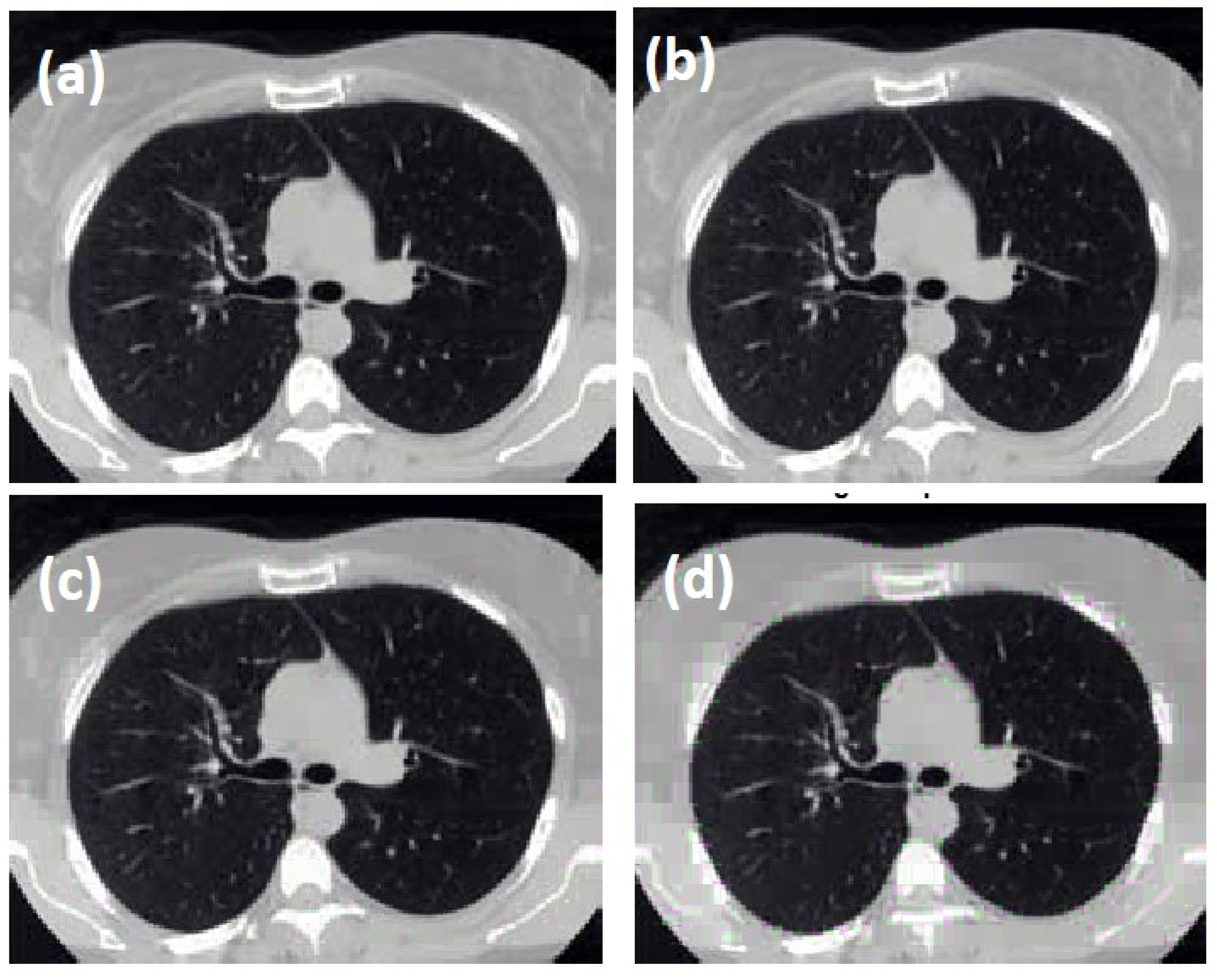
3.4. Medical Image Compression

The proposed algorithm for image compression is simulated using the same targeted device, given in Table 3, used for radix-4. The considered medical image was compressed using different tolerance values, such as 0.0007625, 0.003246, 0.013075 and 0.03924, and it also returns the drop values calculated using the formula given in Equation (7) as 0.10, 0.31, 0.61 and 0.83, respectively, as shown in Figure 24 and Figure 25.

4. Conclusions

In this article, a new high-speed DIT-FFT algorithm based on the radix-4 algorithm for medical image compression was proposed and simulated on a target device xc3s500e-5fg320. The simulation results show that radix-4 processes the input with less delay. From the time delay table, it is very clear that approximately 75% of the processing time is saved with less memory usage. The proposed radix algorithm also showed lower power consumption than the existing radix2, which allows the use of the present algorithm in the medical field, where low-power devices are preferable. This is another milestone for this article. Due to these advantages, the proposed algorithm is used in medical image compression. We observed different tolerances and their drop ratios. It is observed that the scaling factor for image compression depends on tolerance as directly proportional. According to the obtained results for different tolerances, such as 0.0007625, 0.003246, 0.013075 and 0.03924, the drop values are 0.10, 0.31, 0.61 and 0.83, respectively. The level of compression and tolerance values for medical images can be chosen based on the drop ratio and application. Before being taken for ASIC, it can be tested on FPGA for speed and further embedding of the required components.