On the Stability of Collinear Libration Points in the Three-Body Problem with Two Radiating Masses ^†

Abstract

The stability of cloud accumulations of gas and dust particles in the field of binary star systems is studied. As a dynamic model, we consider a restricted three-body problem in which both main bodies are radiating. We study the stability of collinear libration points (CLL) in a nonlinear formulation. The problem of CLP stability is considered in three-dimensional parametric space. It is shown that at the resonance of the fourth order in the plane problem, the points under study are stable in the sense of Lyapunov. In this case, the invariant normal form and Markeev’s theorem are used. The stability of the CLP in the spatial problem is considered. The Birkhoff normal form is used and the Arnold–Moser theorem is used. Results are obtained on stability for most initial conditions (in the Lebesgue measure) and formal stability.

1. Introduction

In photogravitational celestial mechanics, along with the forces of Newtonian attraction $F_g$, the light pressure is taken into account $F_p,$ coming from the radiating body (star) [1]. In some cases, the luminous flux is so intensive that the force $F_p$ competes with gravity $F_g$, and can be even greater than that.

For a particular particle, the magnitude of the light pressure force depends not only on the power of the radiation source (star), but also on the cross-sectional area, the mass and the reflectivity of the particle. To determine the connection between the parameters of the star and the particle, a coefficient Q is introduced, called the particle mass reduction coefficient. For a particular particle, Q has a constant value that characterizes its susceptibility to radiation. The relationship between the parameters of the star [2] and the particle gives the reduction coefficient Q

$$Q=1-(1-\epsilon )A\frac{E}{fM}$$

(1)

(f is the gravitational parameter of the star, E and M is the mass and power of the star, A is a windage of the particle, determined by the ratio of the cross–sectional area to its mass, $\epsilon$ is the coefficient of light reflection). Sufficiently large and dense particles with small values of the parameters A and $\epsilon$ are most affected by the gravitational force of the star, therefore, $Q>0$. For the smallest particles with high windage and reflection coefficient, the action of light is greater than gravity $(Q<0).$

The photogravitational three-body problem introduced by V.V. Radzievskiy [3] has become a good dynamic model for studying the motion of microparticles in binary star systems.

In the elliptical version of the problem (when the orbits of a stellar pair are elliptical), we write the equations of motion of a particle in a rectangular system rotating together with the stars in the form

$$\ddot{x}-2\dot{y}=\frac{\partial W}{\partial x},\ddot{y}+2\dot{x}=\frac{\partial W}{\partial y},\ddot{z}=\frac{\partial W}{\partial z}$$

(2)

where $x,y,z$ are dimensionless coordinates related to the distance $r=p/(1+ecosv)-1$ between the stars (p and e are the focal parameter and the eccentricity of the relative orbital motion of the stellar pair) that are the rectangular coordinates of the particle and W is the force function of the system, equal to

$$W={(1+ecosv)}^{-1}[(x^2+y^2-z^{2}ecosv)/2+Q_1(1-\mu )/R_1+Q_2\mu /R_2]$$

$$R_1={[{(x+\mu )}^2+y^2+z^2]}^{1/2},R_2={[{(x-1+\mu )}^2+y^2+z^2]}^{1/2}$$

(3)

Here, $\mu$ and $1-\mu$ are the dimensionless masses of the stars, and $Q_1$ and $Q_2$ are the reduction coefficients of their mass, which represent the ratio of the difference between the gravitational and repulsive forces to the gravitational force. In terms of physical meaning, numerical values $Q_1$ and $Q_2$ do not exceed 1. For the classical problem $Q_1=1$, $Q_2=1$ (no radiation of bodies) [4].

Libration points—constant solutions of the adopted system of dynamic equations—represent relative equilibria in a circular problem and periodic motions in an elliptic problem. They are found from the system of equations

$$\frac{\partial W}{\partial x}=0, \frac{\partial W}{\partial y}=0, \frac{\partial W}{\partial z}=0,$$

(4)

CLP are located on a straight line connecting the main bodies, and for them $y=0, z=0.$ Their positions on the abscissa axis are determined from the first equation of the system (4). The triangular libration points were carefully studied in [5]. The stability of triangular points in strictly nonlinear formulation were considered in [6,7]. In [8,9], the nonlinear analysis of stable coplanar libration points that are not on the plane of orbital motion of main bodies was completed.

2. Collinear Libration Points and Their Stability in a Plane Problem

The CLP coordinate is determined from the following equation

$$f\left(x\right)=x-Q_1\frac{(1-\mu )(x+\mu )}{{|x+\mu |}^3}-Q_2\frac{\mu (x+\mu -1)}{{|x+\mu -1|}^3}=0$$

(5)

Equation (5) contains three mutually independent parameters $\mu ,Q_1,Q_2.$ Therefore, the problem can consider a three-parameter family of CLPs. Let us consider the case when both components of the binary star radiate and move in circular orbits. From Equation (5), we obtain

$$f^{\prime }\left(x\right)=1+2a\left(x\right), a=Q_1\frac{1-\mu }{{|x+\mu |}^3}+Q_2\frac{\mu }{{|x+\mu -1|}^3}$$

Thus, there is a parameter a [10], which is included in the characteristic equation

$${\lambda }^4+(2-a){\lambda }^2-(1-a)(1+2a)=0,$$

(6)

its solutions are equal to

$${\lambda }_{\alpha }^2=\frac{1}{2}(a-2\pm \sqrt{(9a-8)a},\alpha =1,2$$

When changing the parameter values a in the intervals $8/9<a\le 1$ and $-0.5<a\le 0$, roots ${\lambda }_{\alpha }$ are purely imaginary, and at the boundaries there are multiples. Therefore, the parameter values indicated above by the inequalities correspond to the stability region of libration points in the first approximation. In [11], they constructed diagrams of CLP stability.

In the problem, resonances of the third and fourth orders are found; for third-order resonances, the resonant values of the parameter a have the form $a_{\pm }^{*}=41/108\pm 5\sqrt{145}/108$; for fourth-order resonances, $a_{\pm }=(68+60\sqrt{5})/209.$ As expected, the resonance of the third order leads to the instability of the CLP [12].

In [13], it is shown that at the resonance of the fourth order, the CLPs are stable by Lyapunov.

Below, we consider the stability of the CLP in the spatial problem. The Birkhoff normal form is used, and the Arnold–Moser theorem [14] is applied.

3. Equations of Motion and Expansion of the Hamilton Function

Particle motion $P(x,y,z)$ is given by the canonical equations

$$\frac{d\overline{q_i}}{dt}=\frac{\partial H}{\partial {\overline{p}}_i},\frac{d\overline{p_i}}{dt}=-\frac{\partial H}{\partial {\overline{q}}_i},(i=1,2,3)$$

(7)

where $q_i$ are the Cartesian coordinates of the particle $P(x,y,z),\overline{p_i}$ are the corresponding canonical momenta and $H(x,y,z,\overline{p_1},\overline{p_2},\overline{p_3})$ is the Hamilton analytic function with respect to coordinates and momenta, which, in our case, has the form

$$\begin{array}{c}H=\frac{1}{2}({\overline{p}}_1^2+{\overline{p}}_2^2+{\overline{p}}_3^2)+({\overline{p}}_{1}y-{\overline{p}}_{2}x)-Q_1(1-\mu )/R_1-Q_2\mu /R_2\\ R_{\alpha }={\sqrt{(x-x_{\alpha }}}^2+y^2+z^2,(\alpha =1,2)\end{array}$$

(8)

Here, $Q_1$ and $Q_2$ are coefficients of reduction of the masses of the main bodies, which, in the case of CLP, can take both positive and negative values [10].

We study the stability of the CTL under the assumption that the orbit of the main bodies is circular and the particle P of infinitely small mass at the initial moment of time experiences initial perturbations that take it out of the plane of rotation of the main bodies $S_1$ and $S_2$.

We introduce perturbations into Equation (1) according to the formulas

$$\begin{array}{c}x=x*+q_1,y=q_2,z=q_3,{\overline{p}}_1={\overline{p}}_1^{*}+p_1,{\overline{p}}_2=p_2,{\overline{p}}_3=p_3\\ p_1^{*}=x*,p_2^{*}=y*=p_3^{*}=z_0^{*}=0,\end{array}$$

(9)

where

$$\begin{array}{c}x*=0.5(Q_1^{\frac{2}{3}}-Q_2^{\frac{2}{3}}-1)-\mu ,{\overline{p}}_1^{*}=\mp 0.5\sqrt{2(Q_1^{\frac{2}{3}}+Q_2^{\frac{2}{3}})-(Q_1^{\frac{2}{3}}-Q_2^{\frac{2}{3}})-1}.\end{array}$$

(10)

Expanding the Hamilton function in a row according to the degrees of perturbations and in the neighborhood of the considered collinear point, taken as the origin, we obtain

$$\begin{array}{c}H=H_2+H_3+H_4+\dots \end{array}$$

(11)

Here, $H_m$ are homogeneous polynomials of degree $m(m=2,3,4,...)$ with respect to generalized coordinates and impulses $p_i$, so

$$\begin{array}{c}{H}_m={\displaystyle \sum _{v+l=m}}{h}_{v_1{v}_2{v}_3{l}_1{l}_2{l}_3}·q_1^{v_1}{q}_2^{v_2}{q}_3^{v_3}{p}_1^{l_1}{p}_2^{l_2}{p}_3^{l_3}\end{array}$$

(12)

Then, in Equation (11), the forms $H_2,H_3$ and $H_4$ taking into account (9) will take the following form:

$$\begin{array}{c}{H}_2=\frac{1}{2}(p_1^2+p_2^2+p_3^2)+p_1{q}_2-p_2{q}_1+h_{200}{q}_1^2+h_{020}q{2}^2+h_{002}{q}_3^2+h_{110}{q}_1{q}_2\\ +h_{101}{q}_1{q}_3+h_{001}{q}_2{q}_3,\end{array}$$

(13)

$$\begin{array}{c}{H}_3=h_{300}{q}_1^3+h_{030}{q}_2^3+h_{300}{q}_3^3+h_{210}{q}_1^2{q}_2+h_{201}{q}_1^2{q}_3+h_{120}{q}_1{q}_2^2+h_{021q_2^2{q}_3}\\ +h_{102}{q}_1{q}_3^2+h_{012}{q}_2{q}_3^2+h_{111}{q}_1{q}_2{q}_3,\end{array}$$

(14)

$$\begin{array}{c}{H}_4=h_{400}{q}_1^4+h_{040}{q}_2^4+h_{004}{q}_3^4+h_{310}{q}_1^3{q}_2+h_{130}{q}_1{q}_2^3\\ +h_{103}{q}_1{q}_3^3+h_{301}{q}_1^3{q}_3+h_{031}{q}_2^3{q}_3+h_{013}{q}_3^3{q}_2+h_{211}{q}_1^2{q}_2{q}_3\\ +h_{121}{q}_1{q}_2^2{q}_3+h_{112}{q}_1{q}_2{q}_3^2+h_{220}{q}_1^2{q}_2^2+h_{202}{q}_1^2{q}_3^2+h_{022}{q}_2^2{q}_3^2,\end{array}$$

(15)

where

$$\begin{array}{c}{h}_{200}=-8a,h_{020}=4a,h_{002}=4a,h_{110}=0,h_{101}=0,h_{011}=0\\ h_{300}=16b,h_{120}=-16b,h_{102}=-16b,h_{030}=0,h_{003}=0,h_{210}=0,\\ h_{201}=0,h_{021}=0,h_{012}=0,h_{111}=0,\\ h_{400}=-32c,h_{040}=-12c,h_{004}=-12c,h_{220}=32c,h_{202}=32c,\\ h_{022}=-8c,h_{310}=0,h_{130}=0,h_{103}=0,h_{301}=0,h_{031}=0,\\ h_{013=0},h_{211}=0,h_{121}=0,h_{112}=0.\end{array}$$

(16)

$$\begin{array}{c}a=\frac{Q_1(1-\mu )}{|Q_1^{2/3}-Q_2^{2/3}{+1|}^3}+\frac{Q_2\mu }{|Q_1^{2/3}-Q_2^{2/3}{-1|}^3},\\ b=\frac{Q_1(1-\mu )(Q_1^{2/3}-Q_2^{2/3}+1)}{|Q_1^{2/3}-Q_2^{2/3}{+1|}^5}+\frac{Q_2\mu (Q_1^{2/3}-Q_2^{2/3}-1)}{|Q_1^{2/3}-Q_2^{2/3}{-1|}^5}\\ c=\frac{Q_1(1-\mu )}{|Q_1^{2/3}-Q_2^{2/3}{+1|}^5}+\frac{Q_2\mu }{|Q_1^{2/3}-Q_2^{2/3}{-1|}^5}\end{array}$$

(17)

4. Stability of CLP in a Spatial Problem

The question of the stability of the investigated spatial CLPs can be considered as a stability problem of equilibrium positions $q_i=p_i=0(i=1,2,3)$ of an autonomous Hamiltonian system with three degrees of freedom. As can be seen from (13), here we have the case when $H_2$ is not a sign-definite function, and the characteristic equation of the system has no roots with a nonzero real part. Hence, the stability of the complete system does not follow from the stability of a linear system.

Expanding the Hamilton function into a power series $q_i,p_i$ in the vicinity of the considered equilibrium position, first the Hamiltonian $H_2$ is transformed to the normal form in the form

$$\begin{array}{c}{K}_2={\omega }_1{r}_1-{\omega }_2{r}_2+{\omega }_3{r}_3.\end{array}$$

(18)

The structure of the normal form depends on the type of resonance relation

$$\begin{array}{c}{\omega }_1{r}_1-{\omega }_2{r}_2+{\omega }_3{r}_3=0\left(\right|k_1|+k_2+|k_3|\le 4),\end{array}$$

(19)

where the frequencies of the principal oscillations for the libration points are equal to

$$\begin{array}{c}{\omega }_1=\sqrt{(2-a+\sqrt{(9a-8)a})/2},{\omega }_2=\sqrt{(2-a-\sqrt{(9a-8)a})/2},{\omega }_3=\sqrt{a}.\end{array}$$

(20)

As can be seen from the last expression, for the frequency of spatial oscillations, the parameter a can take only positive values. Therefore, resonances containing the frequency of spatial oscillations can be realized only in a limited part of the region ($8/9<a\le 1$ and $-1/2<a\le 0$) for necessary stability conditions of the system. Let us investigate the stability of CLP at two-frequency resonances. For CLP, the following two-frequency resonances turned out to be possible:

$$\begin{array}{c}{\omega }_1=2{\omega }_2,{\omega }_1=3{\omega }_2,2{\omega }_1={\omega }_3,3{\omega }_1={\omega }_3,2{\omega }_2={\omega }_3,3{\omega }_2={\omega }_3\end{array}$$

Resonances ${\omega }_1=2{\omega }_2$ and ${\omega }_1=3{\omega }_2$, discovered in the plane problem, were studied in [12,13]. In the spatial photogravitational problem, resonances of the third and fourth orders turned out to be possible

$$\begin{array}{c}2{\omega }_1={\omega }_3,3{\omega }_1={\omega }_3,2{\omega }_2={\omega }_3,3{\omega }_2={\omega }_3\end{array}$$

which respectively correspond to the values of the parameter a defined as

$$\begin{array}{c}a=4(1+2\sqrt{7})/27,a=4(-1+\sqrt{10})/9,a=(63+\sqrt{53217})/304,a=(63+\sqrt{53217})/304\end{array}$$

Note that the last two resonances, $3{\omega }_1={\omega }_3$ and $3{\omega }_2={\omega }_3$, match. To construct resonance curves (in the stability region in the linear approximation of the system) for the corresponding specific resonance value of the coefficient a, a curve is constructed, which is determined by the expression

$$\begin{array}{c}\frac{Q_1(1-\mu )}{|Q_1^{2/3}-Q_2^{2/3}{+1|}^3}+\frac{Q_2\mu }{|Q_1^{2/3}-Q_2^{2/3}{-1|}^3}=a\end{array}$$

At resonance $2{\omega }_1={\omega }_3$ (which does not involve the frequency of plane oscillations), which corresponds to the value of the parameter $a=4(1+2\sqrt{7})/27$, the normalized Hamiltonian takes the form [14]

$$\begin{array}{c}H=2{\omega }_1{r}_1-{\omega }_1{r}_3+A({\omega }_1,{\omega }_3)r_3\sqrt{r_1}sin({\phi }_1+2{\phi }_3)+O{(r_1+r_3)}^2,\end{array}$$

(21)

where $A({\omega }_1,{\omega }_3)=-\sqrt{{\omega }_1(x_{1002}^2+y_{1002}^2})$ and the coefficients $x_{1002}$ and $y_{1002}$ look like

$$\begin{array}{c}{x}_{1002}=-\frac{{\omega }_1{h}_{0111}}{2{\omega }_1}-\frac{h_{1002}}{2}+\frac{h_{1200}}{2{\omega }_1^2},y_{1002}=-\frac{{\omega }_1{h}_{0012}}{2}-\frac{{\omega }_1{h}_{0210}}{2{\omega }_1^2}+\frac{h_{1101}}{2{\omega }_1},\end{array}$$

which, for collinear points, are equal to

$$\begin{array}{c}{x}_{1002}=-\frac{h_{1200}}{2{\omega }_1^2},y_{1002}=0\end{array}$$

(22)

hence, the expression

$$\begin{array}{c}A({\omega }_1,{\omega }_3)=-\sqrt{{\omega }_1(x_{1002}^2+y_{1002}^2)}=-\sqrt{{\omega }_1}{x}_{1002}\end{array}$$

is not equal to zero anywhere; therefore, according to the Arnold–Moser theorem, at a third-order resonance from the stability region, in the first approximation, we can say that the CTLs are unstable. If there is a fourth-order resonance in the system, corresponding to the value of the parameter $a=(63+\sqrt{53217})/304,$ using the Birkhoff transformation in the original Hamiltonian, we annihilate the terms of the third degree. The Hamiltonian normalized in this case in polar coordinates will take the following form [13]:

$$\begin{array}{c}H=3{\omega }_1{r}_1-{\omega }_1{r}_3+c_{20}{r}_1^2+c_{11}{r}_1{r}_3+c_{02}{r}_3^2+\\ B({\omega }_1,{\omega }_3)r_3\sqrt{r_1{r}_3}cos({\phi }_1+3{\phi }_3)+O{(r_1+r_3)}^{5/2},\end{array}$$

(23)

where

$$\begin{array}{c}B({\omega }_1,{\omega }_3)=\frac{1}{3}{\omega }_3\sqrt{3(x_{1003}^2+y_{1003}^2)}\end{array}$$

It is important to notice that in the classical problem for a fixed value $\mu$, the coefficients $B({\omega }_1,{\omega }_3),c_{200},c_{100}$ and $c_{020}$ take constant values (which simplifies the investigation of the problem). In this problem, the same coefficients do not remain constant and are functions of arbitrary coefficients of the coefficients $Q_1$ and $Q_2$, which makes the task much more difficult. These are denoted by the coefficients of the Hamiltonian (23)

$$\begin{array}{c}{N}_1=c_{200}+3c_{110}+9c_{020},N_2=3\sqrt{3}B({\omega }_1,{\omega }_3),\end{array}$$

where

$$\begin{array}{c}B({\omega }_1,{\omega }_3)=\frac{1}{3}{\omega }_3\sqrt{3(x_{1003}^2+y_{1003}^2)}\end{array}$$

is defined by expressions

$$\begin{array}{c}{x}_{1003}=\frac{1}{2}{\omega }_1{h}_{0013}+\frac{1}{2{\omega }_3^3}{h}_{1300}-\frac{1}{2{\omega }_3}{h}_{1102}-\frac{{\omega }_1}{2{\omega }_3^2}{h}_{0211}\\ -\frac{9}{5}(x_{0120}\ast x_{0012}+y_{0120}\ast y_{0012})-\frac{1}{{\omega }_3}(x_{1002}{y}_{1011}+x_{1011}{y}_{1002})\\ +\frac{4}{{\omega }_3^2}(x_{1002}{x}_{0201}+y_{1002}{y}_{0201})+\frac{3}{2}(x_{0003}{x}_{0111}+y_{0003}{y}_{0111}),\\ y_{1003}=-\frac{{\omega }_1}{2{\omega }_3}{h}_{0112}+\frac{1}{2}{h}_{1003}+\frac{1}{2{\omega }_3^2}{h}_{1201}+\frac{{\omega }_1}{2{\omega }_3^3}{h}_{0310}\\ -\frac{9}{5}(x_{0120}\ast y_{0012}+x_{0012}\ast y_{0120})-\frac{1}{{\omega }_3}(y_{1011}{y}_{1002}-x_{1011}{x}_{1002})\\ +\frac{4}{{\omega }_3^2}(x_{0201}{y}_{1002}+x_{1002}{y}_{0201})+\frac{3}{2}(x_{0111}{x}_{0003}+x_{0003}{y}_{0111}),\end{array}$$

where coefficients

$$\begin{array}{c}{h}_{0013},h_{1300},h_{1102},h_{0211},h_{0112},h_{1003},h_{1201},h_{0310},x_{0120},y_{0120},\\ x_{1011},y_{1002},y_{1011},x_{0012},y_{0111},x_{0201},y_{0201},x_{0003},x_{0003}\end{array}$$

given for CLP above (16) take values equal to zero, therefore, they are identically equal to zero $x_{1003}$ and $y_{1003}$. Then, the equality takes place

$$\begin{array}{c}{N}_2=3\sqrt{3}B({\omega }_1,{\omega }_3)=0.\end{array}$$

Let us now define the value $N_1=c_{200}+3c_{110}+9c_{020}.$ Here, the coefficients $c_{200},c_{110}{c}_{020},$ which are invariants of the Hamilton function (11) with respect to canonical transformations, depend on the coefficients $h_{v_1{v}_2{l}_1{l}_2}$ that are homogeneous polynomials (12) of degree $m(m=3,4),$ which are equal to

$$\begin{array}{c}{c}_{200}=\frac{3}{2{\omega }_1^2}{h}_{4000}-\frac{27}{8}{\omega }_2^2{y}_{0030}^2-\frac{3}{2}{x}_{1020}^2,\\ c_{110}=\frac{1}{{\omega }_1{\omega }_2}{h}_{2200}-\frac{2}{3}{x}_{1002}^2+\frac{3}{10}{\omega }_2^2{y}_{0012}^2+2x_{0111}{x}_{1020},\\ c_{020}=\frac{3}{2{\omega }_2^2}{h}_{0400}-\frac{1}{6}{x}_{0111}^2-\frac{3}{40}{\omega }_2^2{y}_{0012}^2,\end{array}$$

(24)

where

$$\begin{array}{c}{y}_{0030}=-\frac{1}{{\omega }_1^2}{h}_{3000},x_{1020}=-\frac{3}{2{\omega }_1^2}{h}_{3000},x_{1002}=\frac{1}{2{\omega }_2^2}{h}_{1200},\\ y_{0012}=\frac{1}{{\omega }_1{\omega }_2^2}{h}_{1200},x_{0111}=\frac{1}{{\omega }_1{\omega }_2}{h}_{1200}\end{array}$$

(25)

Substituting from (16) the values $h_{3000}=16b$, $h_{1200}=-16b$ in (24), we have

$$\begin{array}{c}{c}_{200}=-\frac{48}{{\omega }_1^2}c-\frac{864{\omega }_2^2}{{\omega }_1^2}{(1+\frac{1}{{\omega }_1^2})}^2{b}^2-96{(1-\frac{3}{{\omega }_1^2})}^2{b}^2,\\ c_{110}=\frac{32}{{\omega }_1{\omega }_2}c-\frac{96}{{\omega }_2^4}{b}_2+\frac{384}{5{\omega }_1^2{\omega }_2^2}{b}^2-\frac{256}{{\omega }_1{\omega }_2}(1-\frac{3}{{\omega }_1^2})b^2,\\ c_{020}=-\frac{18}{{\omega }_2^2}c-\frac{32}{3{\omega }_2^4}{b}^2-\frac{96}{5{\omega }_1^2{\omega }_2^2{b}^2}\end{array}$$

(26)

where $a,b$ and c are parameters that depend on reduction factors $Q_1$ and $Q_2$ and dimensionless mass parameter $\mu$. As the calculations showed, the modulus of the expression $N_1=c_{200}+3c_{110}+9c_{020}$ is always different from zero. Consequently, the inequality holds everywhere $|N_1|>N_2=0$, which, according to [13], guarantees the existence of Lyapunov stability. 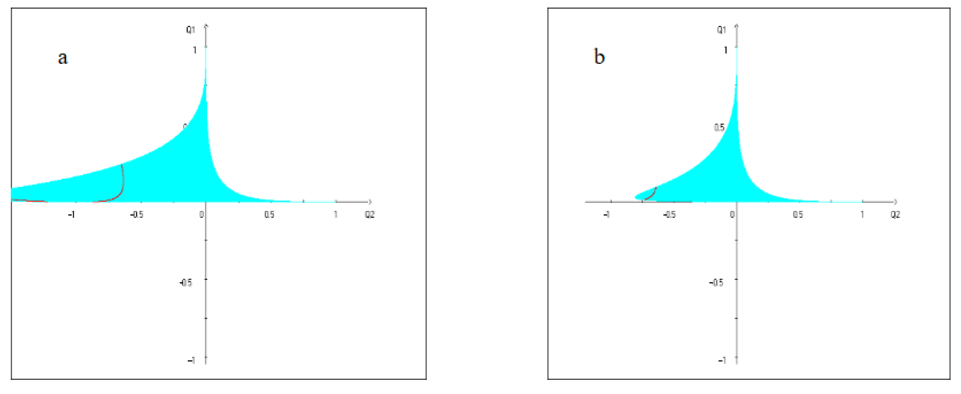In a similar way, it is proved that at a resonance of the third order $2{\omega }_2={\omega }_3$, CLPs are unstable, and at a fourth-order resonance $3{\omega }_2={\omega }_3$ they are stable by Lyapunov. Below are the regions of the stability of the linear system (colored), in which the resonance curves of the fourth order are indicated $2{\omega }_2={\omega }_3$ for two values of the mass parameter $\mu$.

At $\mu =0.001$, the resonance curve is located closer to the middle of the stability region (Figure 1a). When the mass $\mu$ increases up to 0.01 (Figure 1b), the region becomes slightly smaller and the resonance curve becomes closer to the boundary of the stability region and becomes less noticeable than when $\mu =0.001$. Apparently, this fact confirms the above conclusion that resonances containing the frequency of spatial oscillations can be realized only in a limited part ($8/9<a$), being the area of necessary conditions for the stability of CLP.

Note that in the classical problem for a fixed value $\mu$, the coefficients $c_{200},c_{110},c_{020}$ are constants (which much simplifies the investigation of the problem). However, in this problem, the same coefficients are not constants but functions of the coefficients $Q_1$ and $Q_2$, which makes the task much more difficult.

If a ${\omega }_i$ does not satisfy condition (19), then after applying the Birkhoff transformation, the Hamiltonian of the perturbed motion in polar coordinates normalized to the fourth order inclusive has the form

$$\begin{array}{c}H*=K_2(r_1,r_2,r_3)+K_4(r_1,r_2,r_3)\end{array}$$

(27)

Here, $K_4$ is defined by the expression

$$\begin{array}{c}{K}_4=c_{200}{r}_1^2+c_{110}{r}_1{r}_3+c_{0}11r_2{r}_3+c_{002}{r}_3^2\end{array}$$

(28)

Now, we use Arnold’s results on the stability of Hamiltonian systems for most of the initial conditions [13]. It is known that the instability found in the plane problem remains such in the spatial problem.

Assuming that there are no resonances in the system $2{\omega }_1={\omega }_3,{\omega }_1=2{\omega }_2,$${\omega }_1=3{\omega }_2,3{\omega }_1={\omega }_3,2{\omega }_2={\omega }_3,3{\omega }_2={\omega }_3,$ consider a fourth-order determinant

$$\begin{array}{c}{D}_4=det\left|\begin{array}{cc}\frac{{\partial }^2{K}_4}{\partial r_i\partial r_j}& \frac{\partial K_2}{\partial r_i}\\ \frac{\partial K_2}{\partial r_j}& 0\end{array}\right|\end{array}$$

(29)

Expanding the determinant (29), we have

$$\begin{array}{c}{D}_4={\omega }_1^2(c_{011}^2-4c_{020}{c}_{002}+{\omega }_2^2(c_{{101}^2}-4c_{200}{c}_{002})+\\ +{\omega }_3^2(c_{110}^2-4c_{200}{c}_{020})+2{\omega }_1{\omega }_2(c_{101}{c}_{011}-2c_{002}{c}_{110})-\\ -2{\omega }_1{\omega }_3(c_{001}{c}_{110}-2c_{020}{c}_{101})+2{\omega }_2{\omega }_3(c_{110}{c}_{101}-2c_{200}{c}_{011})\end{array}$$

(30)

The balance position $q_i=p_i=0$ is stable for most initial conditions (by the Lebesgue measure) when the determinant $D_4\ne 0$. After using numerical analysis, we check the validity of the inequality $D_4\ne 0$. We see that in the spatial photogravitational three-body problem, the collinear libration points are stable for most initial conditions (by the Lebesgue measure) for all a (except for the values corresponding to internal resonances of the third $2{\omega }_1={\omega }_3$ and $2{\omega }_2={\omega }_3$ and fourth ${\omega }_1=3{\omega }_2,2_1=3{\omega }_3,3{\omega }_2={\omega }_3$ orders) from the stability region in the linear approximation.

The presence of stability in the system for most of the initial conditions means, with a probability close to unity, that the KTLs are stable in the spatial problem.

As shown by numerical calculations, CLPs are formally stable for almost all values of the parameters from the stability region in the linear approximation. The exceptions are, in addition to the values of the parameters corresponding to the studied resonance, perhaps those values $\mu ,Q_1,Q_2$ from the stability region, at which resonances above the fourth order are realized.

The presence of formal stability means that Lyapunov instability is not detected over a practically very long time interval. This suggests that the particles will stay near the stable libration points for quite a long time.