Reinforcement Learning for Solving Control Problems in Robotics ^†

Abstract

The use of reinforcement learning technology for the optimal control problem solution is considered. To solve the optimal control problem an evolutionary algorithm is used that finds control to ensure the movements of a control object along different trajectories with approximately the same values of the quality criterion. Additional conditions for passing the trajectory in the neighbourhood of given areas of the state space are included in the quality criterion. To build a stabilization system for the movement of an object along a given trajectory, machine learning control by symbolic regression is used. An example of solving the optimal control problem for a quadcopter is given.

1. Introduction

The optimal control problem with phase constraints often has a multi-modal functional. Therefore, with its numerical solution by direct approach, it is possible to obtain several control functions that ensure the movement of the object along different trajectories in the state space with approximately the same value of the control quality criterion which is close to the optimal.

A numerical solution to the optimal control problem leads to some difficulties. As a rule, in most optimal control problems, it is necessary to minimize not one but at least two criteria, reach the control goal or minimize the error of reaching the terminal state and still minimize the given quality criterion. Addition of weight coefficients into criteria does not significantly simplify the problem, since the problem of choosing weights arises.

Another search problem is defined as the loss of unimodality of the functional on the space of parameters of the approximating function. Even a piecewise linear approximation of the control function, when only one parameter needs to be found on each interval for each control component, does not guarantee the presence of a single minimum of the goal functional on the space of parameters.

The problem becomes more complicated in the presence of phase constraints that describe the areas of state space forbidden for the optimal trajectory. It is most likely that due to these reasons, and despite numerous attempts [1,2], a universal computational method for the optimal control problem has not been created.

Further studies have shown that if a strictly optimal solution is not needed and solutions close to the optimal are quite satisfactory, then evolutionary algorithms can be successfully applied to the optimal control problems [3].

Sometimes in practice the researcher knows how the object should move along the optimal trajectory, i.e., approximately knows the areas in the state space the optimal trajectory should pass through. If we introduce additional requirements in the form of passing through the given areas into the quality criterion, then the evolutionary algorithm should change the search area and look for a solution that satisfies the additional requirements. This approach is effective when using evolutionary algorithms. Due to the inheritance property, the improvement of the criterion value at each generation is performed on the basis of small evolutionary transformations of possible solutions to the previous generation. Therefore, if at some generation one of the possible solutions passes through the required areas specified by the researcher, then with a high probability the evolutionary algorithm will search for the optimal solution that preserves the obtained properties. A similar technique is used in machine learning with reinforcement [4,5], when the researcher awards the object by the change of the target functional value for the right actions. Currently, reinforcement learning is actively used in the practice of solving control problems [6]. The paper contains a formal description and practical application of reinforcement learning for solving the optimal control problem.

2. The Optimal Control Problem and Reinforcement Learning

Consider a formal statement of the optimal control problem.

The mathematical model of a control object is given in the Cauchy form of an ordinary differential equation system

$$\dot{\mathbf{x}}=\mathbf{f}(\mathbf{x},\mathbf{u}),$$

(1)

where $\mathbf{x}$ is a state space vector, $\mathbf{u}$ is a control vector, $\mathbf{x}\in {\mathbb{R}}^n$, $\mathbf{u}\in \mathrm{U}\subseteq {\mathbb{R}}^m$, and $\mathrm{U}$ is a compact set.

The initial state is given by

$$\mathbf{x}\left(0\right)={\mathbf{x}}^0\in {\mathbb{R}}^n.$$

(2)

The terminal state is given by

$$\mathbf{x}\left(t_f\right)={\mathbf{x}}^f\in {\mathbb{R}}^n,$$

(3)

where $t_f$ is the time to reach the terminal state (3). Time $t_f$ is not given, but it is limited to $t_f\le t^{+}$, where $t^{+}$ is a given positive value.

The quality criterion is given by

$$J=\underset{0}{\overset{t_f}{\int }}{f}_0(\mathbf{x},\mathbf{u})dt\to \underset{\mathbf{u}\in \mathrm{U}}{min}.$$

(4)

Assume that the researcher knows the areas in the state space of where the optimal trajectory should be. Then, additional conditions are included in the quality criterion

$$J_1=\underset{0}{\overset{t_f}{\int }}{f}_0(\mathbf{x},\mathbf{u})dt+p\sum _{i=1}^r{\psi }_i\left(\mathbf{x}\left(t\right)\right)\to \underset{\mathbf{u}\in \mathrm{U}}{min},$$

(5)

where

$${\psi }_i\left(\mathbf{x}\right)=\vartheta (\underset{t}{min}\{\parallel {\mathbf{z}}^i-\mathbf{x}\parallel \}-{\epsilon }_i\left)\right(\underset{t}{min}\{\parallel {\mathbf{z}}^i-\mathbf{x}\parallel \}-{\epsilon }_i),$$

(6)

p is a penalty coefficient, and $\vartheta \left(\alpha \right)$ is a Heaviside step function

$$\vartheta \left(\alpha \right)=\left\{\begin{array}{c}1,\mathrm{if}\alpha >0\hfill \\ 0,\mathrm{otherwise}\hfill \end{array}\right.,$$

(7)

${\epsilon }_i$, $i=1,\dots ,r$ are given small positive values, and ${\mathbf{z}}^i$, $i=1,\dots ,r$ are the centres of known areas.

According to the introduced additional conditions, if an optimal trajectory does not pass near some given point ${\mathbf{z}}^i$, then value of criterion (5) will grow.

3. Computation Experiment

Consider the optimal control problem for the spatial movement of a quadcopter. The mathematical model of the control object is

$$\begin{array}{ccc}\hfill {\dot{x}}_1& =& x_4,\hfill \\ \hfill {\dot{x}}_2& =& x_5,\hfill \\ \hfill {\dot{x}}_3& =& x_6,\hfill \\ \hfill {\dot{x}}_4& =& u_4(sin\left(u_3\right)cos\left(u_2\right)cos\left(u_1\right)+sin\left(u_1\right)sin\left(u_2\right)),\hfill \\ \hfill {\dot{x}}_5& =& u_{4}cos\left(u_3\right)cos\left(u_1\right)-g_c,\hfill \\ \hfill {\dot{x}}_6& =& u_4(cos\left(u_2\right)sin\left(u_1\right)-cos\left(u_1\right)sin\left(u_2\right)sin\left(u_3\right)),\hfill \end{array}$$

(8)

where $g_c=9.80665$.

Control is constrained

$$u_i^{-}\le u_i\le u_i^{+},i=1,\dots ,4,$$

(9)

where $u_1^{-}=-\pi /12$, $u_1^{+}=\pi /12$, $u_2^{-}=-\pi$, $u_2^{+}=\pi$, $u_3^{-}=-\pi /12$, $u_3^{+}=\pi /12$, $u_4^{-}=0$ and $u_4^{+}=12$.

The initial state is given by

$${\mathbf{x}}^0={\left[050000\right]}^T.$$

(10)

The terminal state is given by

$${\mathbf{x}}^f={\left[10510000\right]}^T.$$

(11)

The phase constraints are given by

$${\phi }_k\left(\mathbf{x}\right)=r_k-\sqrt{{(x_1-x_{k,1})}^2+{(x_3-x_{k,3})}^2}\le 0,$$

(12)

where $k=1,2$, $r_1=r_2=2$, $x_{1,1}=2.5$, $x_{1,3}=2.5$, $x_{2,1}=7.5$, $x_{2,3}=7.5$.

It is necessary to find a control function, taking into account the constraints in (9), that minimizes the following criterion

$$J_1=t_f+p_1\sum _{k=1}^2\underset{0}{\overset{t_f}{\int }}\vartheta \left({\phi }_k\left(\mathbf{x}\right)\right)dt\to \underset{\mathbf{u}\in \mathrm{U}}{min},$$

(13)

where $t_f\le t^{+}=5.6$, $p_1=3$.

To solve the control problem numerically, let us use a piecewise linear approximation. The time axis is divided into equal intervals $\Delta t$, and the search for constant parameters is performed at the interval boundaries for each control component. Control is a piecewise linear function that consists of segments connecting points at the bounds of intervals. Given the control constraints, the desired control function is as follows

$$u_i=\left\{\begin{array}{c}{u}_i^{+},\mathrm{if}{\widehat{u}}_i\ge u_i^{+}\hfill \\ u_i^{-},\mathrm{if}{\widehat{u}}_i\le u_i^{-}\hfill \\ {\widehat{u}}_i,\mathrm{otherwise}\hfill \end{array}\right.,i=1,\dots ,4,$$

(14)

where

$${\widehat{u}}_i=d_{i+(j-1)m}+(d_{i+jm}-d_{i+(j-1)m})\frac{t-(j-1)\Delta t}{\Delta t},i=1,\dots ,4,j=1,\dots ,K,$$

(15)

and K is a number of time interval boundaries

$$K=⌊\frac{t^{+}}{\Delta t}⌋+1=⌊\frac{5.6}{0.4}⌋+1=15.$$

(16)

When solving the problem by a direct approach, the condition of reaching the terminal state is included in the quality criterion

$$J_2=t_f+p_1\sum _{k=1}^2\underset{0}{\overset{t_f}{\int }}\vartheta \left({\phi }_k\left(\mathbf{x}\right)\right)dt+p_2\parallel {\mathbf{x}}^f-\mathbf{x}\left(t_f\right)\parallel \to \underset{\mathbf{u}\in \mathrm{U}}{min},$$

(17)

where $p_2=1$,

$$t_f=\left\{\begin{array}{c}t,\mathrm{if}t\le t^{+}\mathrm{and}\parallel {\mathbf{x}}^f-\mathbf{x}\left(t\right)\parallel \le \epsilon =0.01\hfill \\ t^{+},\mathrm{otherwise}\hfill \end{array}\right..$$

(18)

To solve the problem, a hybrid evolutionary algorithm [7] is used.

Figure 1 and Figure 2 show projections on the horizontal plane $\{x_1;x_3\}$ of the two found optimal trajectories. The big circles present the phase constraints in (12).

The criterion for the solutions found had the following values: for the solution in Figure 1 $J_2=5.6434$, for the solution in Figure 2 $J_2=5.6330$.

As can be seen from the experiment, the values of the criteria practically coincide, the solutions found ensure the movement of the object from the given initial state (10) to the given terminal state (11) without violation of the phase constraints. In the series of experiments, the hybrid evolutionary algorithm found solutions that bypass the phase constraints either from above, as in Figure 1, or from below, as in Figure 2.

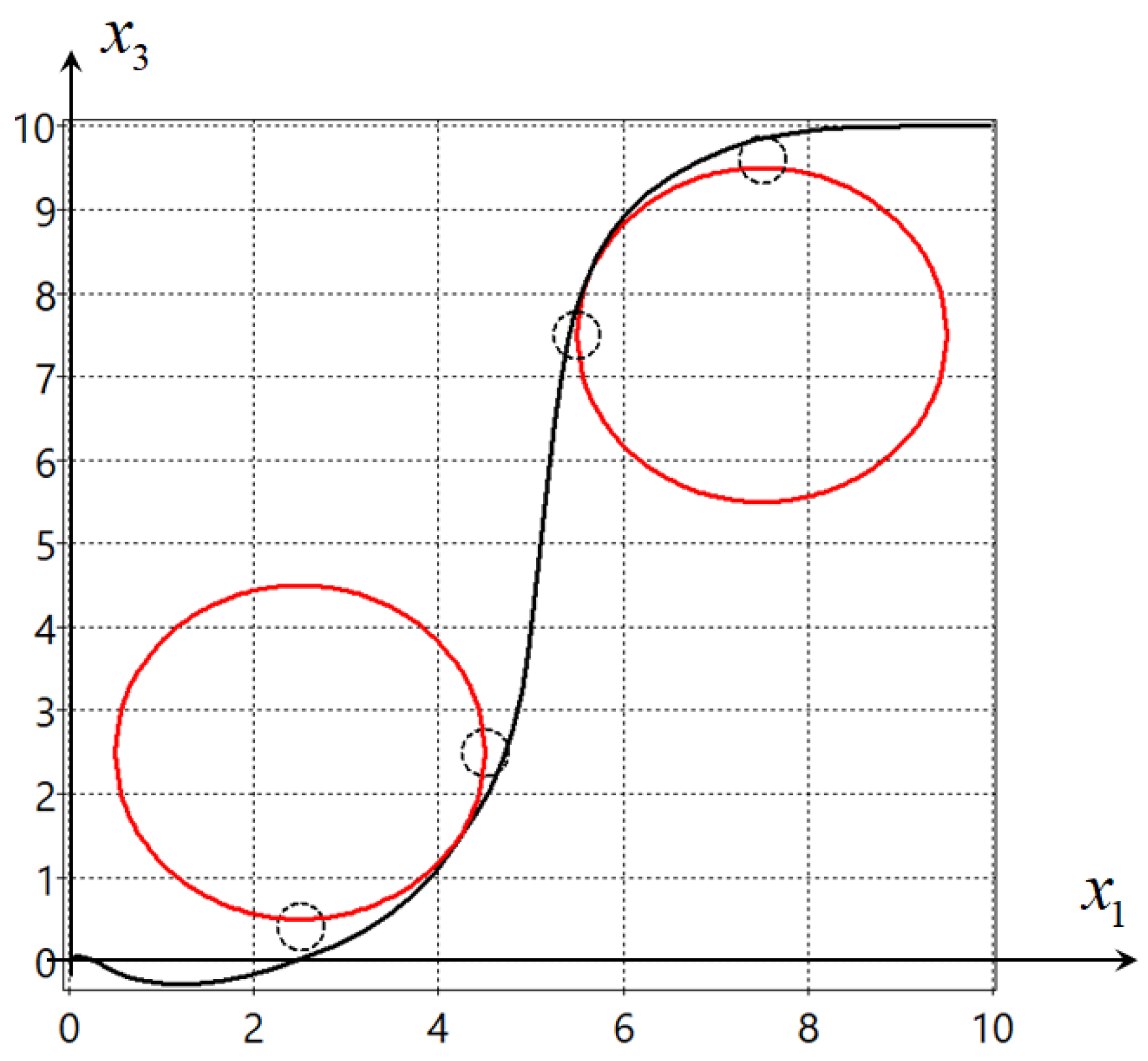
Suppose that we need the control object to move between obstacles. For this purpose the desired areas on the horizontal plane are defined. It is known that in the presence of interfering phase constraints, the optimal trajectory should be close to the boundary of these constraints. For the given problem four desired areas are defined as

$$\begin{array}{c}{\mathbf{z}}^1={\left[2.50.4\right]}^T,{\epsilon }_1=0.6,\\ {\mathbf{z}}^2={\left[4.52.5\right]}^T,{\epsilon }_2=0.6,\\ {\mathbf{z}}^3={\left[5.57.5\right]}^T,{\epsilon }_3=0.6,\\ {\mathbf{z}}^4={\left[7.59.6\right]}^T,{\epsilon }_4=0.6.\end{array}$$

(19)

The conditions for passing through the desired areas (19) are included in the quality criterion

$$J_3=t_f+p_1\sum _{k=1}^2\underset{0}{\overset{t_f}{\int }}\vartheta \left({\phi }_k\left(\mathbf{x}\right)\right)dt+p_2\parallel {\mathbf{x}}^f-\mathbf{x}\left(t_f\right)\parallel +p_3\sum _{i=1}^4{\psi }_i\left(\mathbf{x}\right)\to \underset{\mathbf{u}\in \mathrm{U}}{min},$$

(20)

where $p_3=3$.

The hybrid evolutionary algorithm found the following optimal solution $\mathbf{d}={[d_1\dots d_{60}]}^T=[-11.1092$, $5.9957$, $-0.0532$, $7.0045$, $17.5091$, $18.1172$, $-1.6764$, $18.7012$, $-16.0121$, $10.5543$, $-19.9307$, $12.1721$, $-6.0892$, $0.5339$, $-0.8616$, $19.2556$, $-13.7218$, $15.1266$, $0.3982$, $14.2650$, $-1.1768$, $2.9832$, $4.3286$, $15.1508$, $-8.9240$, $-19.6814$, $4.5363$, $15.9879$, $-0.0026$, $1.1203$, $13.2592$, $-6.6358$, $-6.2012$, $-0.5328$, $-0.0354$, $4.2548$, $11.6764$, $-4.3345$, $-6.7336$, $19.8643$, $0.3360$, $-8.9741$, $-2.6648$, $12.5608$, $19.6577$, $-19.9308$, $-1.6252$, $19.3797$, $-1.1954$, $2.2625$, $5.9582$, $16.0807$, $-0.8272$, $2.3167$, $0.9842$, $14.2695$, $-6.3767$, $2.3895$, $0.3742$, ${16.2710]}^T$.

Figure 3 shows the projection of the found optimal trajectory for the solution with quality criterion $J_3=5.5730$. Small dashed circles are the desired areas, while big circles are the constraints.

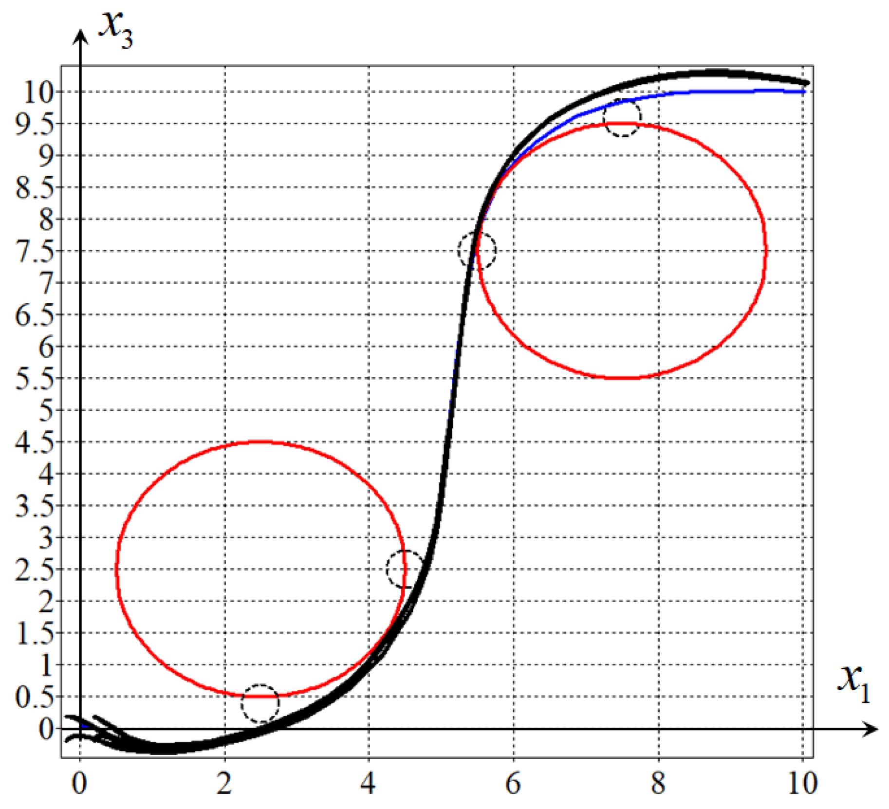
To implement the obtained solution according to the extended statement of the optimal control problem, it is necessary to build a system to stabilize the movement of the object along the optimal trajectory [8]. For this purpose, machine learning control is used [9]. The control function structure search is carried out by symbolic regression [10].

The obtained solution is

$$u_i=\left\{\begin{array}{c}{u}_i^{+},\mathrm{if}{\tilde{u}}_i\ge u_i^{+}\hfill \\ u_i^{-},\mathrm{if}{\tilde{u}}_i\le u_i^{-}\hfill \\ {\tilde{u}}_i,\mathrm{otherwise}\hfill \end{array}\right.,i=1,\dots ,4,$$

(21)

where

$${\tilde{u}}_1=\mu \left(G\right),$$

(22)

$${\tilde{u}}_2=({\tilde{u}}_1-{\tilde{u}}_1^3){\rho }_{17}(A+\mu \left(G\right))\vartheta \left(F\right){\rho }_{17}(x_4^{*}-x_4),$$

(23)

$${\tilde{u}}_3={\tilde{u}}_2+tanh\left({\tilde{u}}_1\right)+{\rho }_{19}(A+\mu \left(G\right))+{\rho }_{17}\left(W\right),$$

(24)

$$\begin{array}{ccc}\hfill {\tilde{u}}_4& =& {\tilde{u}}_3+ln\left|{\tilde{u}}_2\right|+\mathrm{sgn}(A+\mu \left(G\right))\sqrt{|A+\mu (G\left)\right|}+{\rho }_{19}\left(A\right)+arctan\left(C\right)+\hfill \\ \hfill & & \mathrm{sgn}\left(E\right)+arctan\left(F\right)+exp\left(q_2(x_2^{*}-x_2)\right)+\sqrt{q_1},\hfill \end{array}$$

(25)

$$A=B\mathrm{sgn}\left(D\right)\sqrt{\left|D\right|}tanh\left(D\right)exp\left(H\right),B=exp\left(C\right)+{\rho }_{17}\left(F\right)+cos\left(q_6(x_6^{*}-x_6)\right),$$

$$C=D+tanh\left(E\right)+{\rho }_{18}\left(V\right),D=E+\sqrt[3]{F}+sin\left(W\right),$$

$$E=F+G+exp\left(H\right)-V,F=H+\mathrm{sgn}(x_5^{*}-x_5)+{(x_2^{*}-x_2)}^3,$$

$$G=q_6(x_6^{*}-x_6)+q_3(x_3^{*}-x_3)+\mathrm{sgn}(x_2^{*}-x_2)\sqrt{|x_2^{*}-x_2|},$$

$$H={\rho }_{17}(q_6(x_6^{*}-x_6)+q_3(x_3^{*}-x_3))+V^3+W+q_6{q}_5^2{(x_5^{*}-x_5)}^2+{(x_5^{*}-x_5)}^2,$$

$$V=sin\left(q_6(x_6^{*}-x_6)\right)+q_5(x_5^{*}-x_5)+q_2(x_2^{*}-x_2)+cos\left(q_1\right)+exp(x_5^{*}-x_5)+\vartheta (x_2^{*}-x_2),$$

$$W=q_4(x_4^{*}-x_4)+q_1(x_1^{*}-x_1)+sin\left(q_6\right),$$

$$\mu \left(\alpha \right)=\left\{\begin{array}{c}\alpha ,\mathrm{if}\left|\alpha \right|\le 1\hfill \\ \mathrm{sgn}\left(\alpha \right),\mathrm{otherwise}\hfill \end{array}\right.,{\rho }_{17}\left(\alpha \right)=\mathrm{sgn}\left(\alpha \right)ln\left(\right|\alpha |+1),$$

$${\rho }_{18}\left(\alpha \right)=\mathrm{sgn}\left(\alpha \right)(exp(\left|\alpha \right|)-1),{\rho }_{19}\left(\alpha \right)=\mathrm{sgn}\left(\alpha \right)exp(-|\alpha \left|\right),$$

where $q_1=13.02930$, $q_2=11.21509$, $q_3=15.91016$, $q_4=14.33447$, $q_5=14.67798$, $q_6=9.91431$ and ${\mathbf{x}}^{*}={[x_1^{*}\dots x_6^{*}]}^T$ is a state vector of the reference model.

Figure 4 shows the trajectories from eight initial states on the horizontal plane.

4. Results

The paper presents the use of machine learning technology with reinforcement to solve the optimal control problem with phase constraints using an evolutionary algorithm. To implement reinforcement learning, additional conditions defining the form of the optimal trajectory are introduced into the quality criterion. The optimal trajectory should pass through specified areas whose positions depend on the phase constraints. An example of solving the optimal control problem for a quadcopter by machine learning with reinforcement was given.

5. Discussion

The use of reinforcement learning technology to solve the optimal control problems of robotic devices is advisable, since in most cases the developer approximately knows the form of the optimal trajectory for the problem being solved.

References

1. Rao, A.V. A Survey of Numerical Methods for Optimal Control. Adv. Astronaut. Sci. 2010, 135, 497–528. [Google Scholar]
2. Grachev, N.I.; Evtushenko, Y.G. A Library of Programs for Solving Optimal Control Problems. USSR Comput. Math. Math. Phys. 1980, 2, 99–119. [Google Scholar] [CrossRef]
3. Diveev, A.I.; Konstantinov, S.V. Study of the Practical Convergence of Evolutionary Algorithms for the Optimal Program Control of a Wheeled Robot. J. Comput. Syst. Sci. Int. 2018, 4, 561–580. [Google Scholar] [CrossRef]
4. Brown, B.; Zai, A. Deep Reinforcement Learning in Action; Manning, Publications Co.: Shelter Island, NY, USA, 2019; 475p. [Google Scholar]
5. Morales, M. Grokking Deep Reinforcement Learning; Manning Publications Co.: Shelter Island, NY, USA, 2020; 472p. [Google Scholar]
6. Duriez, T.; Brunton, S.; Noack, B.R. Machine Learning Control–Taming Nonlinear Dynamics and Turbulence; Springer: Cham, Switzerleand, 2017; 229p. [Google Scholar]
7. Diveev, A. Hybrid Evolutionary Algorithm for Optimal Control Problem. In Lecture Notes in Networks and Systems; Springer: Berlin/Heidelberg, Germany, 2023; Volume 543, pp. 726–738. [Google Scholar]
8. Diveev, A.; Sofronova, E. Synthesized Control for Optimal Control Problem of Motion Along the Program Trajectory. In Proceedings of the 2022 8th International Conference on Control, Decision and Information Technologies (CoDIT), Istanbul, Turkey, 17–20 May 2022; pp. 475–480. [Google Scholar]
9. Diveev, A.I.; Shmalko, E.Y. Machine Learning Control by Symbolic Regression; Springer: Cham, Switzerleand, 2021; 155p. [Google Scholar]
10. Koza, J.R.; Keane, M.A.; Streeter, M.J.; Mydlowec, W.; Yu, J.; Lanza, G. Genetic Programming IV. Routine Human-Competitive Machine Intelligence; Springer: Boston, MA, USA, 2003; 590p. [Google Scholar]
Figure 1. Projection of optimal trajectory 1 on the horizontal plane.
Engproc 33 00029 g001
Figure 2. Projection of optimal trajectory 2 on the horizontal plane.
Engproc 33 00029 g002
Figure 3. Projection on the horizontal plane of the optimal trajectory found by reinforcement learning.
Engproc 33 00029 g003
Figure 4. Projection on the horizontal plane of the optimal trajectories from eight initial states.
Engproc 33 00029 g004
Disclaimer/Publisher’s Note: The statements, opinions and data contained in all publications are solely those of the individual author(s) and contributor(s) and not of MDPI and/or the editor(s). MDPI and/or the editor(s) disclaim responsibility for any injury to people or property resulting from any ideas, methods, instructions or products referred to in the content.