Abstract
Air traffic management (ATM) requires the handling big data of moving objects, such as flight trajectories. There is, however, a lack of specialized tools for trajectory-data management, where the spatiotemporal data are first class citizens. Instead, specialized algorithms for trajectory-data management are built on top of existing geospatial tools. In this paper, we showcase MobilityDB, which is an open-source database for moving objects. MobilityDB is developed as an extension to PostgreSQL and PostGIS that specializes in the storage and processing of trajectory data. Its data model integrates spatiotemporal and temporal types as first class citizens in the database. It thus allows one to perform complex spatial and spatiotemporal queries. This paper presents how to combine MobilityDB with Grafana, an open-source dashboard tool, to perform basic and advanced queries and interact with Grafana visualization. A use case for flight trajectories, based on the OpenSky Network data, is illustrated.
1. Introduction
Massive amounts of aviation Automatic dependent surveillance–broadcast (ADS-B) trajectories are being continuously collected. Platforms such as OpenSky make them available to support research and development. Data scientists then face the challenge of processing the collected data to extract relevant information. Generally, there is a lack of established tools for movement data management and analysis.
In this paper, we explore the potential of two open-source tools, MobilityDB and Grafana, in building an integrated end-to-end platform for aviation data analysis using publicly available OpenSky data. The implementation includes data loading, data processing, exploratory data analysis, and the creation of a business intelligence dashboard with visualizations of example key-performance indicators (KPIs). MobilityDB’s spatiotemporal data types and functions and Grafana’s visualizations make it possible to generate efficient data queries on the fly with dynamic query parameters controlled by the front-end.
This paper targets data scientists and developers in the aviation domain. It aims to inspire the production of responsive business intelligence dashboards, with feedback between the development environment and end-user experience during exploration.
2. MobilityDB and Grafana Overview
2.1. MobilityDB
MobilityDB [1] is a moving object database, implemented as an extension to PostgreSQL and PostGIS, that introduces temporal and geospatial data types using an abstract data model to represent spatiotemporal data.
Conventionally, data related to a single point in time is stored as a single instance (i.e., a row) with separate attributes (i.e., columns) used to store the data and the timestamp. Representing data that changes over time would thus use multiple instances. MobilityDB’s data model uses an array of (value, timestamp) pairs to represent data changing over time. For example, a temporal integer (i.e., tint), stores a sequence of integers and the corresponding timestamps, resulting in an array structure as a single value (cell) in an entity (table). The base data types integer and timestamps in this array are based on the existing PostgreSQL data types (i.e., int and timestamptz).
These temporal types may be then treated as continuous functions. Redundant values are removed through a lossless normalization process. The data array can thus be exploited by returning not just the known discrete points but also values between two consecutive pairs using a stepwise or linear interpolation.
This same approach is extended to represent temporal geometry points, tgeompoint, which are spatiotemporal data types that leverage the existing PostGIS geometry type. This is the data type used to store an entire flight’s trajectory. MobilityDB also includes functions to efficiently manipulate temporal types, such as intersect(), within(), speed(), and tgeompoint_seq() [2], among others. Additional information can be found in the official MobilityDB reference documents (https://docs.mobilitydb.com/MobilityDB/master/mobilitydb-manual.pdf, accessed on 1 September 2022).
In OpenSky data, each time point is represented as a discrete event. Table 1 shows a sample of the data for a single flight, ANZ1220, on 1 June 2020.

Table 1.
Sample of raw data representation in MobilityDB database for a single flight (ANZ1220) before transformations.
The data is transformed into trajectories using the SQL query in Listing 1. First, we create the composite index icao24_time_index to improve the performance of trajectory generation. The SQL query creating the trajectories uses the same method to create each temporal type value (tonground, taltitude, and tgeom). We explain it next using the tgeom column as an example:
| Listing 1: SQL query to transform raw data into MobilityDB datatypes. |
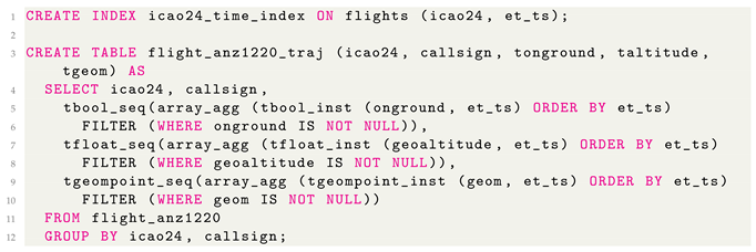 |
- The first (most inner) call is tgeompoint_inst(), which combines each geometry point (lat, long) with the timestamp where that point existed.
- array_agg() aggregates all of the instants together into a single array for the items aggregated by the GROUP BY statement. In this case, it will create an array for each icao24 with a particular callsign.
- Finally, tgeompoint_seq() constructs the array as a sequence that can be manipulated with MobilityDB functions. Equivalent sequence constructor functions are used for other attribute data types (e.g., float uses tfloat_seq()).
The resulting entity contains an instance for each unique icao24-callsign combination with an array for each temporal type value, as seen in Table 2.

Table 2.
Sample of data representation in MobilityDB database for a single flight (ANZ1220) after transformation into trajectories.
This data representation model results in a compression of the data. For a 24-h period of flights, the data entity before trajectory generation was 2531 MB. When the data are transformed to temporal trajectories, where each instance represents a flight, the entity size decreased to 870 MB, almost a 3:1 compression ratio.
2.2. Grafana
Grafana (https://grafana.com/, accessed on 2 January 2023) is an open-source, time-series data query, visualization, and alerting tool [3]. It can unify numerous data sources as it does not require loading data into the tool itself. It has an active community of contributors that develop plugins for new data sources and visualization tools. Grafana proves to be useful for both query development as well as production-quality business intelligence dashboards that support collaborative development and customization. Using a query editor, Grafana allows the user to query and combine data from any connected source and to create visualizations for dashboards, and it has an alerting function if critical thresholds are reached.
Grafana provides a flexible dashboard interface to manipulate data and introduce dynamic variables into queries through a graphic user interface. There are some limitations in Grafana’s capability to visualize geometries, which require additional data transformations for visualization purposes. However, it remains a significant improvement over other common tools such as Quantum Geographic Information Systems (QGIS), an open source visualization software for geographic and spatial data. Additionally, Grafana handles time-series data very effectively.
2.3. Data Pipeline: Combining MobilityDB and Grafana
Given the choice of MobilityDB as the moving object database, it was natural to identify a tool that can work alongside it to visualize the temporal and spatiotemporal results. Grafana was chosen as it is also open-source, is able to connect to PostgreSQL as a back-end database, and is extensible. Grafana supports community developed extensions in the form of JavaScript plugins, enabling the development of potentially missing features.
Grafana was beneficial during data exploration and query development to immediately visualize query results. Using multiple visualization panels, various query iterations were visually compared against each other. On-the-fly query adjustments were made “post-query” to fine tune the visualizations by specifying conditions using Grafana’s options panel. The visualization type was selected in Grafana after query development, and query visualization functioned on simple query returns without needing the use of any SQL statements such as ROLLUP or CUBE.
A limitation of this pipeline is that currently Grafana cannot render lines using geometric coordinates. Grafana also lacks the capabilities to plot data types such as geometry (from PostGIS) and tgeompoint (from MobilityDB). Instead, lines are represented by plotting points and heat maps, which is accomplished with an additional final step in query building to unnest data from an array to discrete points. This results in an increased number of data called from the database and longer rendering times for visualizations.
3. Implementation
3.1. Data Workflow
The process for implementing a mobility dashboard is composed of several steps, described next.
- Clean and Transform DataOpenSky data was loaded into MobilityDB, pre-processed, and coverted into trajectories using MobilityDB temporal types. After this one-time processing step, the database was ready for analysis. Real-time analysis and loading can be accomplished with a script written using an OpenSky Network API (https://openskynetwork.github.io/opensky-api/index.html, accessed on 3 January 2023) that pushes new state vectors into the database as they arrive.
- Create User Queries and Visualization PanelsSQL queries were designed with Grafana variables to make visualization dynamically change with end user’s input. Grafana visualization panels were chosen and visual conditions and options were set. Grafana replaces the variables in the query with user-selected values and pushes the query to the database. MobilityDB completes query processing and returns the result of the query.
- Deploy the Dashboard Responding to User QueriesEnd users can interact with the visualization and do their analysis. They can interact with the data through the Grafana’s graphic user interface (GUI) without needing to make changes to any SQL code. For time-specific filters, the user clicks through time-advancement options and Grafana updates the SQL query and retrieves new data for visualizations. For real-time monitoring, users can specify the query refresh interval as well.
3.2. Building SQL Queries
The dataset used contains flight information over a 24-h period from OpenSky Network (https://opensky-network.org/data/datasets, accessed on 3 January 2023). Each row of raw data represents the attributes at a unique point in time for a particular airframe (i.e., airplane) and is identified by the attribute icao24. Each row also includes an attribute callsign, which is the unique flight identifier assigned by an airline. The methodology and functions used in each query are explained to highlight the unique aspects of MobilityDB and Grafana.
The queries cover the following:
- Section 3.2.1: queries and visualizations without temporal datatypes
- Section 3.2.2: creating and slicing trajectories
- Section 3.2.3: using trajectories with moving object functions
3.2.1. Querying Discrete Points
Query 1: What is the flight path of a single airframe over a user-defined time period?
Listing 2 uses the global variable $__timeFilter() on et_ts (the timestamp value) to create a query that can by updated dynamically by the dashboard user through Grafana’s user interface. Grafana is not currently able to natively visualize trajectories as vectors. The TABLESAMPLE SYSTEM () PostgreSQL function is used to return approximately 5% of the results to reduce the number of discrete points along the trajectory path to return (Figure 1). This is done to improve overall performance without sacrificing the ability to visualize the data.
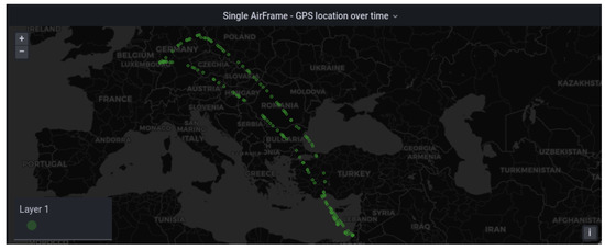
Figure 1.
Visualization of single airframe location in GeoMap panel using discrete points.
| Listing 2: SQL query to return a single airframe flight path over user-defined time period. |
 |
Query 2: What is the altitude and ground speed of flight TRA051?
This query is used to explore some of the differences between the Traffic library and the combination of MobilityDB and Grafana.
Traffic [4] is a Python library that provides numerous functions for flight related analysis and API calls that integrate with OpenSky data. On the other hand, MobilityDB and Grafana are used together for providing value in a few key areas:
- Data analysis using trajectories;
- Improving query development experience;
- Dashboard generation for business intelligence.
The above query can be implemented using the Traffic library as shown in Listing 3 and visualized in Figure 2. Notice that belevingsvlucht is a flight type structure containing flight TRA051.
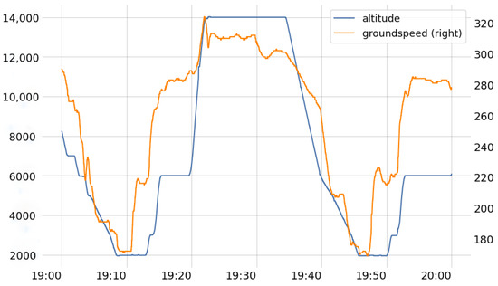
Figure 2.
Multiple variables displayed in dual axis plot with traffic library.
| Listing 3: Python code to return a single airframe’s altitude and ground speed using Traffic library. |
 |
Listing 4 shows the same query executed in MobilityDB. The results of separate queries (Query A and Query B) are combined together in Grafana to show different parameters in the same visualization panel (Figure 3). This query can be further extended by creating a user-defined variable to replace icao24=’c827a6’, allowing the dashboard user to select different (or multiple) airframes from a list in Grafana.

Figure 3.
Interactive graph of velocity and altitude with tooltips on mouse hover.
| Listing 4: SQL query to return a single airframe’s altitude and ground speed using MobilityDB. |
 |
We compare the code and visualization of both approaches.
- Traffic is written in Python, MobilityDB uses SQL (PostgreSQL dialect).
- Traffic loads all data into memory for computation (as it is a Python library). Datasets larger than memory can be handled in Python but need functionality not present by default. MobilityDB is a database so it has capabilities to handle datasets much larger then the memory size.
- Visualization options are coded into traffic before run time; Grafana uses a GUI to manipulate both visualization options and post-processing filters.
- Traffic provides a static plot (e.g., zoom requires code change). Grafana includes user tooltips on mouse hover and dynamic result filtering through GUI selections.
3.2.2. Creating Flight Trajectories
MobilityDB datatypes are used to segment the 24-h airframe trajectories (in temporal columns) based on the time period of when the airframe’s callsign changes to create trajectories for each flight. This generic approach is used whenever there is a need to split one trajectory by the inflection points of a value in time of some other trajectory.
Note that in this case study, a single airplane can complete the same flight path more than once in a 24-h period. A simple GROUP BY icao24, callsign statement would not be sufficient, and the use of additional context-specific conditions such as vertical rate changes or where altitude is 0 would suffer from noise in the data. The incorrect approach would result in two or more distinct flights where the airframe and flight number are the same being included in a single temporal trajectory.
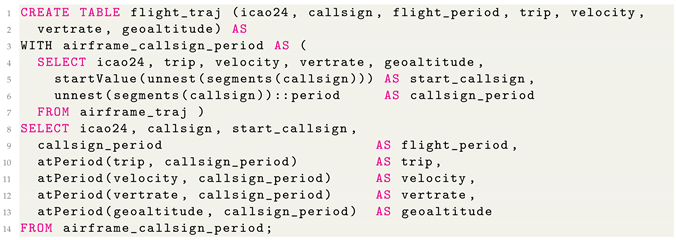
In Listing 5 the airframe_callsign_period table provides the start and end timestamps that will be used to “slice” the other temporal sequences in the airframe trajectory. The function segments(callsign) returns an array of beginning and ending timestamps for when a callsign exists for an airframe. Function unnest() is used to expand the segment array, and each value is cast to a period that is used in the main query. Function atPeriod() creates new temporal sequences that have a start and end timestamp corresponding to callsign_period. This transformation takes place only once, when loading new data into the MobilityDB database; the trajectories are then used directly to query flight specific statistics in Grafana.
| Listing 5: SQL query to create flight trajectories using MobilityDB functions. |
 |
3.2.3. Querying Flight Trajectories
Query 3: What is the average velocity of each flight?
In Listing 6, the twavg() function, which returns a time-weighted average, can be called directly on the temporal float data of each flight trajectory. Error-checking steps and filters such as removing trajectories with missing velocities or incorrect velocity values will reduce the number of datareturned from the database, improving dashboard performance.
| Listing 6: SQL query to return average flight velocity. |
 |
Grafana is used for post-processing, with some modifications to the axis to highlight the resolution of higher ranges (Figure 4). If only the “top 10” results are needed, the SQL query should be modified to return fewer results rather than post-processing in Grafana.
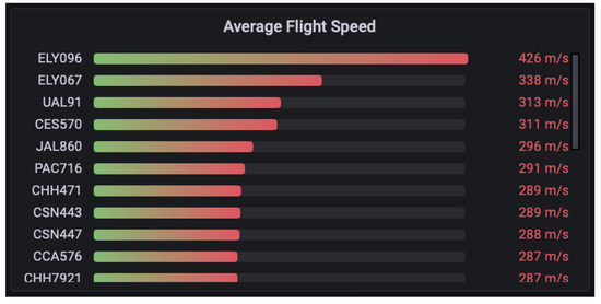
Figure 4.
Average flight velocity from highest to lowest.
3.2.4. Dynamic Variables and Visualizing Beyond Three Dimensions
Query 4: For all flights taking off at any given time, how did the vertical ascent rate change over the course of takeoff?
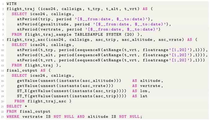
Listing 7 uses the Grafana global variables $__from:date and $__to:date to allow user inputs in the Grafana GUI. The flight_traj_asc table returns the period of the first sequence of each flight. This is done using atRange() to clip the temporal data to create ranges where vertrate is between [1, 20], which represents an ascending airframe. Function sequenceN selects the first of the generated sequences, which is takeoff, the first period an airframe ascends. Function atPeriod is used to return the period (start and end timestamp) of the takeoff sequence. For visualization purposes, the sequence arrays are unpacked in the final_output table using unnest(), which provides a series of discrete points that can be visualized in Grafana (Figure 5a,b). In Grafana, adjustments are made to have the marker size reflect altitude and the color represent vertical ascent rate. A manual override is added for the minimum and maximum vertrate values to make large values more visible. The results have a filter set on a per airframe basis, where a single airframe shows a short increased vertical ascent rate towards the end of the ascent period.
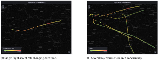
Figure 5.
Grafana visualizations of changing vertical ascent rates and altitudes during take off for (a) a single airframe and (b) multiple airframes.
| Listing 7: SQL query to return vertical ascent rate and altitude during takeoff. |
 |
For concurrent visualizations of multiple air frames, it is important to manage the number of datapoints being returned, or be cognisant of global variable limits, as the user can select a large time frame returning more data than the dashboard designer anticipated.
Query 5: How much airplane traffic is there at Amsterdam at any given time in the day?
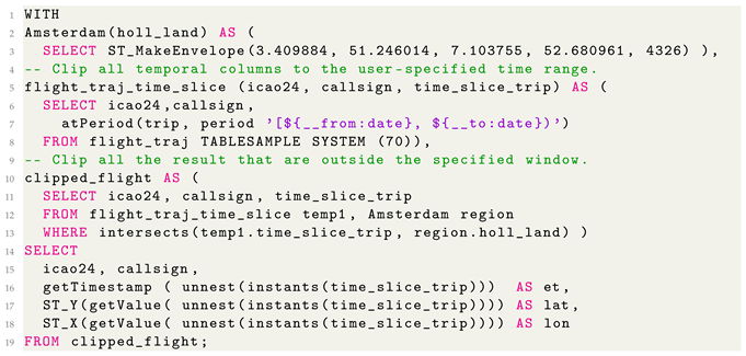
Listing 8 uses functions atPeriod() and intersect() to slice through time and geographic areas. The query returns any trajectory that intersects with the region above Amsterdam. Figure 6 shows that on 1 June 2020 from 10 h to 11 h there is minimal air activity over the region, while from 11 h to 12 h the airspace is much busier. Exploring hours and days visually makes it possible to observe how the occupation of the airspace changes throughout the day. The traffic library does not have the ability to slice through user defined areas, although it does have the ability to import predefined airport areas [5].
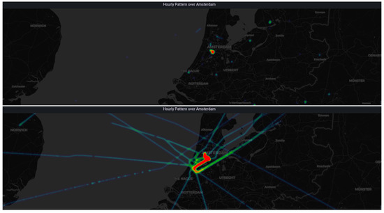
Figure 6.
Heat map of Amsterdam air traffic from 10 h to 11 h (low traffic, top) and from 11 h to 12 h (high traffic, bottom).
| Listing 8: SQL query to return flight paths intersecting the geometric boundary of Amsterdam. |
 |
4. Conclusions and Future Work
This paper presented technology that can be used in an end-to-end platform for storing, querying, analyzing, and visualizing flight trajectories. MobilityDB, an open-source moving object database, was used as an efficient data-management platform. Grafana, an open-source dashboard, was used for interactive spatiotemporal visual analytics. We demonstrated connecting MobilityDB and Grafana to build an air traffic dashboard. Several examples of queries have been presented to showcase the utility of the proposed technology combination.
At the moment, MobilityDB is a generic trajectory database that does not specialize in specific types of trajectories (e.g., vehicles, ships, and aircraft). With these promising results, future work would extend MobilityDB with aircraft-specific analysis functions. Additionally, extending Grafana to visualize trajectories in vector format would result in a significant improvement in performance and consistency when working with big data.
Author Contributions
Conceptualization, M.S. and E.Z.; Methodology, A.B. and M.I.T.; Supervision, M.S. and E.Z.; writing—original draft preparation, A.B. and M.I.T.; writing—review and editing, A.B. and M.I.T. All authors have read and agreed to the published version of the manuscript.
Funding
This research received no external funding.
Institutional Review Board Statement
Not applicable.
Informed Consent Statement
Not applicable.
Data Availability Statement
Data was optained from the OpenSky Network (https://opensky-network.org/data/datasets, accessed on 16 August 2022.)
Conflicts of Interest
Co-authors of this paper, M.S. and E.Z. are co-founders and steering committee members of the MobilityDB project. The paper presents the use of MobilityDB with OpenSky data. The reported results respect the scientific objectivity, and the whole work is repeatable by readers.
References
- Zimányi, E.; Sakr, M.; Lesuisse, A. MobilityDB: A Mobility Database Based on PostgreSQL and PostGIS. ACM Trans. Database Syst. 2020, 45, 1–42. [Google Scholar] [CrossRef]
- Godfrid, J.; Radnic, P.; Vaisman, A.; Zimányi, E. Analyzing public transport in the city of Buenos Aires with MobilityDB. Public Transp. 2022, 14, 287–321. [Google Scholar] [CrossRef]
- Venkatramulu, S.; Phridviraj, M.; Srinivas, C.; Rao, V.C.S. Implementation of Grafana as open source visualization and query processing platform for data scientists and researchers. Mater. Today Proc. 2021; in press. [Google Scholar] [CrossRef]
- Olive, X. Traffic, a toolbox for processing and analysing air traffic data. J. Open Source Softw. 2019, 4, 1518. [Google Scholar] [CrossRef]
- Olive, X.; Basora, L. A Python Toolbox for Processing Air Traffic Data: A Use Case with Trajectory Clustering. In Proceedings of the 7th OpenSky Workshop 2019, Zurich, Switzerland, 21–22 November 2019; EPiC Series in Computing. pp. 73–84. [Google Scholar] [CrossRef]
Disclaimer/Publisher’s Note: The statements, opinions and data contained in all publications are solely those of the individual author(s) and contributor(s) and not of MDPI and/or the editor(s). MDPI and/or the editor(s) disclaim responsibility for any injury to people or property resulting from any ideas, methods, instructions or products referred to in the content. |
© 2023 by the authors. Licensee MDPI, Basel, Switzerland. This article is an open access article distributed under the terms and conditions of the Creative Commons Attribution (CC BY) license (https://creativecommons.org/licenses/by/4.0/).