Simulation of FBG Temperature Sensor Array for Oil Identification via Random Forest Classification ^†

Abstract

Water–oil separation is important in the oil industry, as the incorrect classification of oil can lead to losses in the production and have an environmental impact. This paper proposes the use of fiber Bragg grating (FBG) temperature sensor array to identify the oil in water–emulsion–oil systems, using only the temperature responses for oil classification results in operational and economic benefits. To demonstrate the possibility of using the FBG temperature sensor to classify oil level, the temperature distribution of an oil storage tank, with 2 m height and 0.8 m in diameter, is simulated using thermal distribution models. Then, the temperature effect in a 2 m long FBG array with a different number and distribution of FBGs is simulated using the transfer matrix method. In each case, we extract the wavelength shift ($\Delta \lambda$), total width at half the maximum (FWHM) and the location of the FBG in the fiber. For the oil classification, we dichotomized the fluids into oil and non-oil (water and emulsion). Due to the low separability of the classes, the random forest algorithm was chosen for classification, starting with 200 FBG equidistant sensors and decreasing to 6, with different distributions along the fiber. As expected, the highest accuracy occurs with the 200 FBGs array (96%). However, it was possible to classify the oil with an accuracy of 94.89% with only 8 FBGs, using tests for two proportions (with a significance of 5%); the accuracy of 8 FBGs is the same as of 50 FBGs.

1. Introduction

The water–oil separation is an important process in oil industry [1]. Nowadays, oil is the principal energy source of the world [2]. In the oil extraction, the oil arrives in the tanks combined with water, gas, and sludge. The combination of these components forms the water–oil interface [3]. The effective monitoring, control and separation of oil and water layers in production tanks result in economy on oil production costs and reduction of the environmental pollution [3]. A problem in oil classification is to detect emulsion layers, a region between water and oil in which fluids blend homogeneously [1]. The interface of the tank is organized at sludge at the bottom, water, emulsion, oil, foam, and gas at the top of the tank [3]. For oil production tanks, the main goal is the correct classification of oil. Thus, instead of classifying each fluid of the entire tank, we can just focus on the optimal oil classification. This problem is then reduced to a two-dimensional case: oil and non-oil.

There are several sensors used to identify the water–oil interface as summarized in [1]. However, many of them are electrical conductors or work with electrical signals, which can be unsuitable for classified areas. optical fiber sensors (OFS) are immune to electromagnetic interference, have corrosion resistance and no electrical power needed at the measuring point [1]. A widely used sensor is the fiber Bragg grating (FBG) sensor [4]. Its main advantage is its multiplexing capabilities, allowing a large number of sensors in a single optical fiber cable [4].

FBG temperature sensors can be found in the area of health, construction, and industry in general, as discussed in [5]. This sensor technology is used in the oil industry, due to the temperature variations observed in crude oil tanks. In refractive index [4] and hydrostatic pressure sensors, fluid density [1] can be used for fluid classification. However, these sensors need incorporation in different structures [1] or modifications in the fiber for refractive index sensing [4]. FBGs are naturally sensitive to temperature and strain. Therefore, these sensors also need a temperature sensor. Thus, oil classification using only temperature response results in operational and economic benefits, since there are fewer sensors and easy assembly of the sensor array due to FBG inherent sensitivity to temperature variations [6].

Machine learning algorithms (ML) are divided into three learning groups: supervised, semi-supervised, and unsupervised [7]. Supervised ML algorithms are those of which the possible responses of the problem are known. In unsupervised ML algorithms, on the other hand, the response of the problem uses cluster techniques [8]. Finally, semi-supervised ML algorithms are those where learning is done with supervised and unsupervised inputs, seeking to find grouping and response criteria [9]. The use of OFS in conjunction with ML has been widely employed [10].

This paper presents a simulation study of FBG temperature sensors classification in oil using as low a number of sensors as possible. Temperature distribution in the tank due to solar radiation is simulated. The temperatures obtained along the tank are the input for the FBG temperature variation simulation; the following information was collected: wavelength shift ($\Delta \lambda$), full width at half maximum (FWHM). This work also proposes the identification of the optimal number and location of FBGs using machine learning approaches. The temperature variation is not high inside the tank, as the thermal dynamics with small heat exchange results in a low distinction between the fluids. The RF algorithm was applied to the classification, as it is indicated for data with a low distinction between classes [11].

2. Materials and Methods

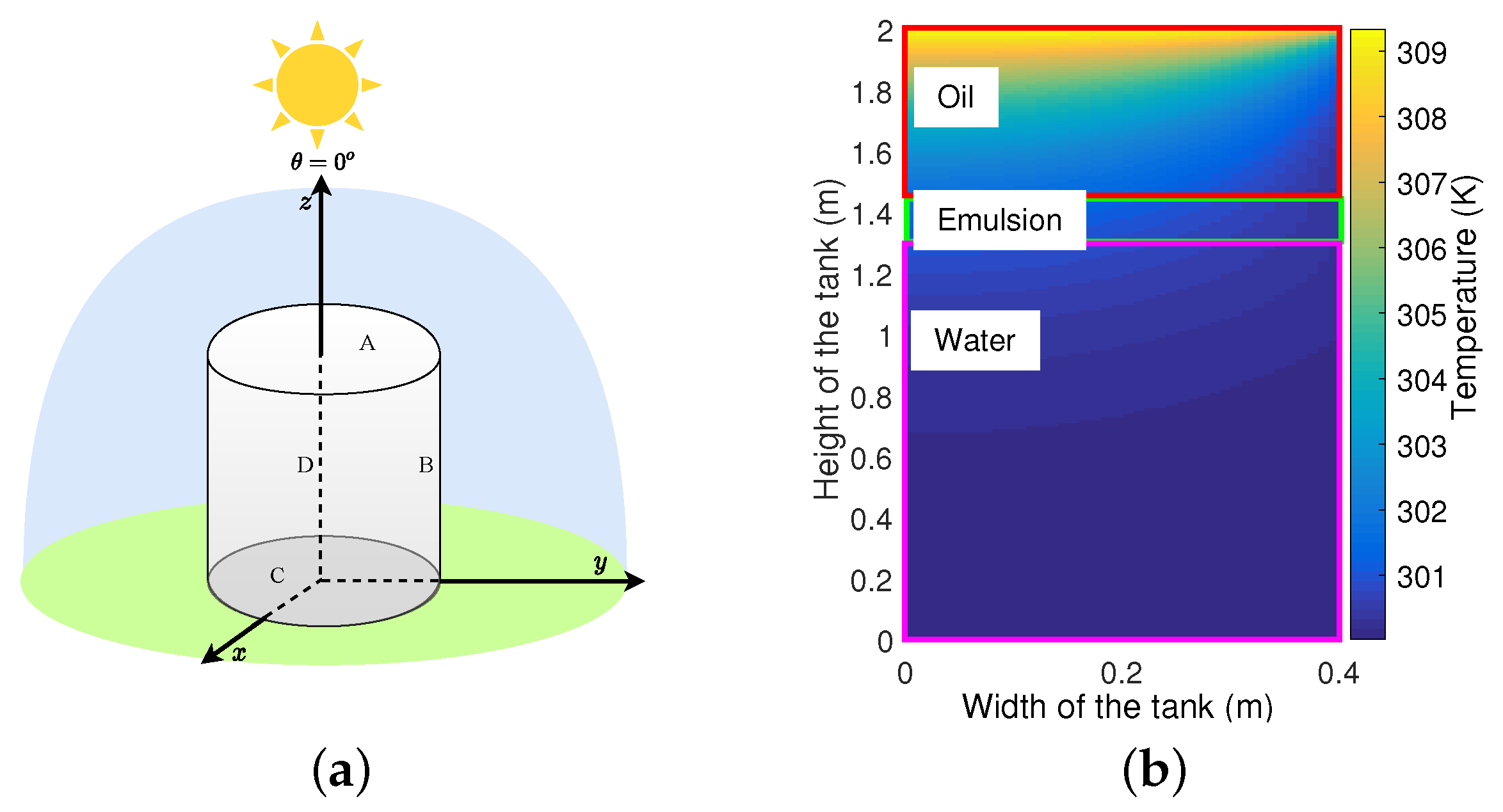
2.1. Simulation Process

A tank with dimensions of 2 m height and 0.8 m diameter is simulated, assuming the presence of solar radiation. Inside the tank, the oil, emulsion and water layers were simulated. In ambient temperature, the thermal conductivity water is 6.13 × 10${}^{-3}$ W/mK and for oil is 1.2 × 10${}^{-3}$ W/mK. For emulsion, we assumed similar quantities of water and oil, thus choosing the arithmetic mean of the thermal conductivities of water and oil, 3.665 × 10${}^{-3}$ W/mK. The solar angulation adopted is 0${}^{\circ }$ to represent midday period with higher radiation, known as sun at zenith. The boundary conditions of the storage tank are shown in Figure 1a. The center of the tank and the bottom are adiabatic, the top receives constant solar radiation, and the tank’s external walls suffer convection with the external environment. The fluid inside the tank is considered to be in a stationary state. Axisymmetric distribution is adopted for the temperature profile. Outside the tank, we assumed white paint on the metallic substrate, which is the emissivity of the tank surface ($\epsilon$) of 0.96, for tanks following Kirchhoff’s law of thermal radiation. The detailed discussion and equations are presented in [12]. To identify the fluid with FBG temperature sensors, we simulate different layers’ heights inside the storage tank, where the total level is always 2 m. The upper and lower bounds of level variations for water are from 0.4 m to 1.6 m. Emulsion varies from 0 m to 0.2 m and oil varies from 0.4 m to 1.6 m in steps of 0.1 m. These variation intervals result in 2331 combinations of oil, emulsion and water. An example of temperature distribution in the oil tank is shown in Figure 1b.

Based on the simulation, the temperature distribution inside the tank, we simulate the presence of FBGs temperature sensor inside it. The fiber is 2 m long and 125 $\mathsf{\mu }$m in diameter, with different FBGs distributions along it. The objective is to correctly identify the oil according to the temperature variations. For this, we analyze $\Delta \lambda$ and FWHM variations. These two parameters vary with the temperature changes in which the fiber is exposed. $\Delta \lambda$ changes due to the effect of thermo-optic and thermal expansion, while FWHM changes due to the effect of chirp in FBG when it is submitted to a nonuniform temperature distribution along the FBG region (with physical length of 10 mm) [6].

For numerical analysis of the FBG temperature sensor into the tank, coupled mode equations with a modified transfer matrix formulation (T-matrix) were used to solve coupled mode equations for a large number of grid segments [13]. We also consider that the temperature is distributed on the z-axis. The temperature distribution on the y and x-axes was ignored, as the fiber diameter (125 $\mathsf{\mu }$m) is much smaller than the tank diameter (0.8 m) and fiber length (2 m). The equations and discussion of coupled mode theory for FBGs are presented in [13]. To solve these equations, the T-matrix approximation is employed. For details and equations, interested readers should refer to [13].

The simulated spectra presented in Figure 2 show that the different temperatures cause differences in the FBG spectrum profile. The observed variations in FWHM are lower than the $\Delta \lambda$. The FBG exposed to a temperature of 300.05 K is represented in Figure 2 by the green curve. If compared to the initial spectrum, in the FWHM, there was a decrease in the fourth decimal. In the pink curve, the FBG was exposed to 302.50 K, and besides the wavelength shift, there was an increase in the FWHM. In the case of the red curve (309.17 K), we observed an increase in wavelength shift and FWHM compared to the initial spectrum, but lower variation in FWHM than that observed at 302.50 K.

To find the ideal number of FBGs and their location, different points were tested based on RF accuracy. In general, FBGs close to tank top have high temperatures due to thermal radiation. High temperatures avoid classification errors, since their increase generates greater difference between classes. For fibers with 25, 50 and 100, due to the large number of FBG location possibilities, we randomly selected 10 sensor distributions in each case. Fibers with 6, 8, 10 and 12 FBGs were selected based on the points that were classified correctly for more times in previous cases.

High temperatures avoid classification errors, as their increase generates a greater difference between classes.

2.2. Random Forest

Random forest is an ensemble-learning algorithm. Algorithms with this learning methodology are more robust and precise than those in which unique learning is considered [14]. This method is similar to decision trees. Its hierarchical form allows considering nonlinear relations in the data to generate classification regions [11]. In RF, different random bootstrap samples are considered for each selected classification tree [11]. The samples are distributed identically, resulting in low error and bias in the classification, thus reducing the total variance of the classification. [11,14].

According to the temperature distribution found in Section 2.1, we dichotomized the classes in oil and non-oil: water and emulsion. Then, with all the possible conditions of fluid variation in the tank, the location of each FBG, $\Delta \lambda$ and the FWHM of the FBGs were extracted. The output of the algorithm is the classification of the oil (and non-oil). Note that all possible temperature distributions have been generated according to the upper and lower bounds previously defined for each layer. To select the ideal number of FBGs, we started with 200 FBGs with equidistant distribution, assuming a 2 m fiber. Then, the number of FBGs was reduced and we changed their locations along the fiber. In addition, to validate the results, cross validation was employed, dividing the samples into training and testing. After the training of the first set of samples, the trained algorithm was applied in the remaining data, those in which the estimated class is equal to the actual class are classified as a success, and the accuracy is the ratio between the success and the total number of estimations. Based on these scores, it was possible to classify or identify the oil.

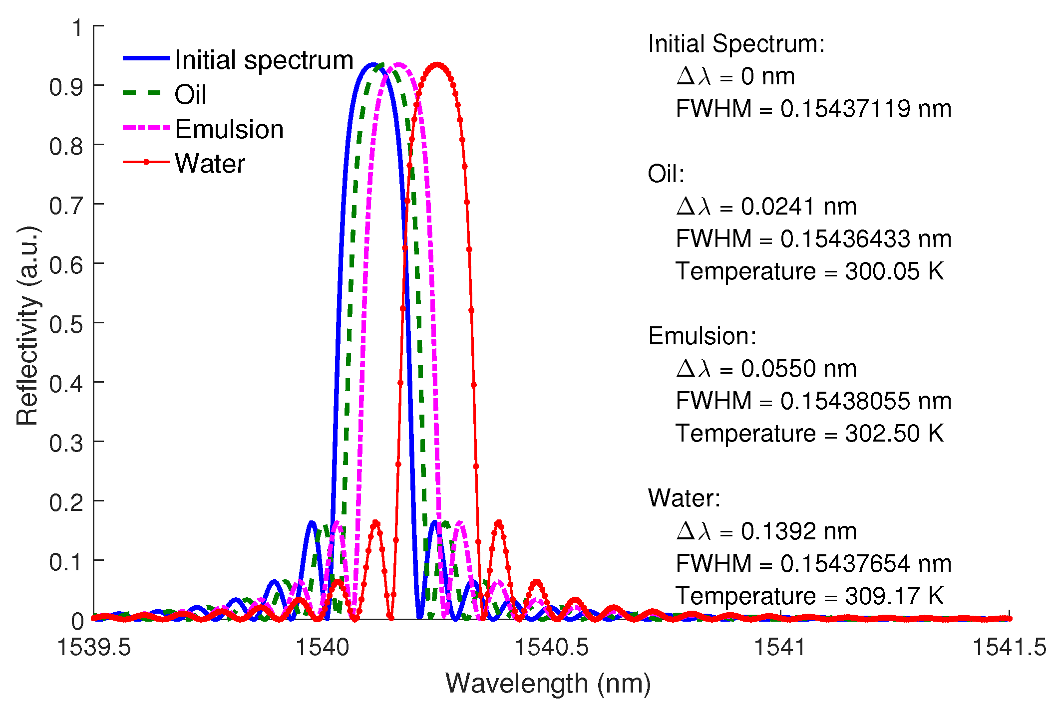
3. Results and Discussion

The interest of the analysis is the correct classification in oil using as low a number of sensors as possible. We started the selection process at 200 equidistant points, then 6, 8, 10, 12, 25, 50 and 100, with different distributions along the fiber and without the requirement of equidistance. The oil and non-oil classification were done by RF, using cross validation, dividing the data in training (65% data, randomly selected), where the classification criteria were taught to the machine and tested (35% remaining) for the classification. For RF forecast, the test data were evaluated in each of the decision trees created by in the training, and associated with the class with the closest characteristics.

The RF input variables were $\Delta \lambda$, FWHM, and the location of the FBG relative to the tank. The expected output in the algorithm was the fluid classification: oil or non-oil. It is also possible to indirectly estimate the oil level based on the classification. Figure 3a shows the association of $\Delta \lambda$ with the classes. Note that only some values above the third quartile of the non-oil class intersect with the oil class. Thus, $\Delta \lambda$ separates almost correctly the two classes. For Figure 3b, the FWHM cannot correctly divide two classes due to the high intersection between classes compared to Figure 3a. Thus, we can assume that the FWHM is less significant than $\Delta \lambda$ for the fluid classification. There is also a lack of symmetry between the median and the first and third quartiles, representing the non-normality of the data for Figure 3a,b. To guarantee that we are not inserting multicollinearity in the model, we calculate the correlation ($\rho$) between FWHM and $\Delta \lambda$, obtaining $\rho$ = 0.29. Based on the observed $\rho$, we verify that there is no increase of variability due to repeated information in RF. To find the ideal number of FBGs and their location, different points were tested based on RF accuracy. As there are a large number of localization possibilities for each case, the locations that resulted in the highest accuracy are presented. In general, the FBGs very close to the top of the tank had high temperatures due to radiation. We assume that the FBGs along the fiber have spatial distribution below 0.1 m, except for 200 FBGs. For fibers with 6, 8, 10, 12, 25, 50 and 100 sensors, because there are a large number of localization possibilities for each case, we randomly selected 10 sensor distributions. Then, the location that returned the highest accuracy in each fiber was selected. Figure 3c shows the accuracy by the number of RF trees with different number of FBGs in the array. The highest accuracy was found with the highest number of FBGs. However, inscribing this many FBGs into the fiber is expensive, and interrogators have limited wavelength ranges. A low number of sensors ensures higher spectral efficiency, because they use a smaller bandwidth of the interrogator. Thus, a high number of sensors, for example, 200, 100 or 50 FBGs, are not efficient options. Reducing the FBGs to 12, we find the average accuracy of 94.88%; with 10 we observe 94.63 and 8 FBGs 94.83. The difference between 8, 10 and 12 FBGs is lower than 0.2%. In reducing to 6 FBGs, there was a 10% lower accuracy, which indicates 8 FBGs as the ideal number.

The classification of oil and non-oil is mutually exclusive, and thus, it has Bernoulli distribution. Hence, the accuracy can be tested with 8 and 25, 50, 100 and 200, using the tests for two proportions. The p-values with a significance of 5% are presented to compare the 8 FBGs array with the other ones. Comparing the accuracy of an 8 FBGs array with the one of 200 FBGs, we obtain a p-value = 0.0003742, at a 5% significance level, which indicates the higher accuracy of the 200 FBGs array. The same occurs with 100 FBGs, with a p-value of 0.007578. However, when comparing the 8 FBG sensor with a 50 FBG sensor and a 25 FBG sensor, we can state that both are significantly equal, with p-values of 0.292 and 0.9888, respectively. Thus, a temperature sensor with 8 FBGs has the same accuracy as sensors with 25 or 50 FBGs. The choice of the distributions in Figure 3d was made by analyzing the scenarios with 25, 50, 100 and 200 FBGs, in the places with FBGs that classified correctly more often. The distributions with less accuracy in Figure 3d have irregular spacing between the FBGs, unlike the distributions with greater accuracy. The location of the FBG influences the observed accuracy.

4. Conclusions

This paper proposes, via simulation, the use of FBG temperature sensors for the identification inside the oil tank. The simulated tank is 2 m in height and 0.8 m in diameter, with influence on solar radiation at a zenith angle. For the analysis, we dichotomize the fluids in oil and non-oil. The algorithm inputs are: $\Delta \lambda$, FWHM and the location of the FBG relative to the tank. $\Delta \lambda$ and FWHM were extracted through numeric simulation in a 2-m fiber with a different spatial distribution and number of FBGs (from 200 to 6). We observed that FWHM has lower influence for the classification than $\Delta \lambda$. The parameters were observed based on the temperature variation fluids inside the tank. The RF algorithm was applied for the classification, since it is indicated for data that have low distinction between the classes. The selection of the ideal number was based on the classification accuracy with respect to the number of FBGs in the fiber. The ideal number of FBGs for the simulation was 8, since it has lower production cost and higher spectral efficiency when compared to 200 or 100 sensor arrays fiber. Then, through the tests for two proportions, it was found that when using 8 FBGs at a 5% significance level, its accuracy is equal to using 25 or 50 FBGs in the sensor array. Future works include direct estimation of fluid level based on the temperature measured by the FBGs.

References

1. Leal-Junior, A.G.; Marques, C.; Frizera, A.; Pontes, M.J. Multi-interface level in oil tanks and applications of optical fiber sensors. Opt. Fiber Technol. 2018, 40, 82–92. [Google Scholar] [CrossRef]
2. Brockway, P.E.; Owen, A.; Brand-Correa, L.I.; Hardt, L. Estimation of global final-stage energy-return- on-investment for fossil fuels with comparison to renewable energy sources. Nat. Energy 2019, 4, 612–621. [Google Scholar] [CrossRef]
3. Atehortúa, C.M.G.; Pérez, N.; Andrade, M.A.B.; Pereira, L.O.V.; Adamowski, J.C. Water-in-oil emulsions separation using an ultrasonic standing wave coalescence chamber. Ultrason. Sonochem. 2019, 57, 57–61. [Google Scholar] [CrossRef] [PubMed]
4. Zhang, B.; Kahrizi, M. High-Temperature Resistance Fiber Bragg Grating. Sensors 2007, 7, 586–591. [Google Scholar] [CrossRef]
5. Rao, Y.J. Recent progress in applications of in-fibre Bragg grating sensors. Opt. Lasers Eng. 1999, 31, 297–324. [Google Scholar] [CrossRef]
6. Da Silva, J.C.C.; Martelli, C.; Kalinowski, H.J.; Penner, E.; Canning, J.; Groothoff, N. Dynamic analysis and temperature measurements of concrete cantilever beam using fibre Bragg gratings. Opt. Lasers Eng. 2007, 45, 88–92. [Google Scholar] [CrossRef]
7. Albalate, A.; Minker, W. Semi-Supervised and Unsupervised Machine Learning: Novel Strategies; ISTE Ltd.: London, UK; John Wiley & Sons: Hoboken, NJ, USA, 2011; p. 320. [Google Scholar]
8. Fallucchi, F.; Luccasen, R.A.; Turocy, T.L. Identifying discrete behavioural types: A re-analysis of public goods game contributions by hierarchical clustering. J. Econ. Sci. Assoc. 2019, 5, 238–254. [Google Scholar] [CrossRef]
9. Dunlop, M.M.; Slepčev, D.; Stuart, A.M.; Thorpe, M. Large data and zero noise limits of graph-based semi-supervised learning algorithms. Appl. Comput. Harmon. Anal. 2019, 1, 1–43. [Google Scholar] [CrossRef]
10. Thaisongkroh, P.; Samartkit, P.; Pullteap, S. Applications of optical fiber sensor technology for prioritized industry in Thailand development strategy: A review. In Proceedings of the Seventh International Conference on Optical and Photonic Engineering (icOPEN 2019), Phuket, Thailand, 16–20 July 2019; Volume 11205, p. 1120511. [Google Scholar]
11. Proniewska, K.; Pregowska, A.; Malinowski, K.P. Identification of Human Vital Functions Directly Relevant to the Respiratory System Based on the Cardiac and Acoustic Parameters and Random Forest. IRBM 2020, in press. [Google Scholar] [CrossRef]
12. Incropera, F.P.; Dewitt, D.P. Fundamentals of Heat and Mass Transfer, 7th ed.; John Wiley & Sons: Hoboken, NJ, USA, 2011. [Google Scholar]
13. Prabhugoud, M.; Peters, K. Modified transfer matrix formulation for Bragg grating strain sensors. J. Lightwave Technol. 2004, 22, 2302–2309. [Google Scholar] [CrossRef]
14. Lee, T.H.; Ullah, A.; Wang, R. Bootstrap Aggregating and Random Forest; Springer: Cham, Switzerland, 2020; Volume 52, pp. 389–429. [Google Scholar]
Figure 1. (a) Oil storage tank layout. A = Tank top (constant heat flow), B = Outside wall (convection with the external environment), C = Bottom (adiabatic wall), D = Axisymmetric (adiabatic). (b) Temperature distribution of the fluid in the tank, with relation figure (a) on zy plane. Oil= 0.55 m, Emulsion= 0.15 m and Water= 1.3 m.
Engproc 02 00020 g001
Figure 2. Fiber Bragg grating (FBG) spectra for three simulated temperature conditions. The initial spectrum is also presented for comparison purposes.
Engproc 02 00020 g002
Figure 3. (a) Box plot of Δ λ for oil and non-oil classification. (b) Box plot of total width at half the maximum (FWHM) for oil and non-oil classification. (c) Number of trees per accuracy in the best prediction based on the RF algorithm. (d) Number of trees per accuracy when using 8 FBGs in different distributions.
Engproc 02 00020 g003
Publisher’s Note: MDPI stays neutral with regard to jurisdictional claims in published maps and institutional affiliations.