Alone We Can Do So Little; Together We Cannot Be Detected ^†

Abstract

It is no longer possible to imagine our everyday life without time series data. This includes, for example, market developments, COVID-19 cases, electricity prices, and other data from a wide variety of domains. An important task in the analysis of these data is the detection of anomalies. In most cases, this is accomplished by examining individual time series. In our work, we use the techniques of cluster analysis to establish a relationship between time series and groups of time series. This relationship allows us to observe the development of time series in their entirety, thereby gaining additional insights. Our approach identifies outliers with a real-world reference and enables the user to locate outliers without prior knowledge. To underline the strengths of our approach, we compare our method with another known method on two real-world datasets. We found that our solution needs significantly fewer calculations, produces more reasonable results, and can be applied to real-time data. Moreover, our method detected additional outliers, whose occurrence could be explained by real events.

1. Introduction

Outlier or anomaly detection in time series is the problem of identifying rare or deviating observations in (univariate or multivariate) time series. Those observations may occur once or form a sequence when arising multiple times in a row. Finding anomalies in time series can be beneficial in a variety of applications, such as fraud detection in stock markets [1,2], anomaly detection in network data [3,4], and the detection of unusual time series in medical data [5,6]. The sheer number of possible applications of anomaly detection in time series makes it important for industry; therefore, it has been implemented in a number of business applications released by Google (https://cloud.google.com/blog/products/data-analytics/ (accessed on 10 April 2022)), RapidMiner (https://rapidminer.com/glossary/anomaly-detection/ (accessed on 10 April 2022)), Microsoft, and IBM [7,8]. The broad diversity of applications and products indicates a variation in the underlying data, which requires specific solutions in order to detect meaningful anomalies. Furthermore, outliers may also be defined differently, depending on the context at hand.

Most approaches focus on the detection of anomalous observations or subsequences in a single time series. This is useful for many applications but does not include a comparison to other time series from the same domain. However, assuming that time series from the same context are influenced by similar framework conditions, such a comparison becomes necessary. The idea of outlier detection by comparing time series is part of recent research and often applies Dynamic Time Warping (DTW) techniques [9,10] or the Granger Causality [11,12]. Although, these approaches are able to identify anomalous data points or even subsequences, they are limited to the comparison of only two time series at a time. The comparison of one time series to a group of other time series at the same time is, therefore, the next logical step; however, it also requires techniques to localize corresponding groups. The latter is well researched and is referred to as cluster analysis in time series.

In general, the goal of cluster analysis is to group objects with the objects in the same group being as similar as possible to each other and the objects from different groups being as dissimilar as possible. The similarity between two objects is usually expressed by a distance function (e.g., Euclidean distance). The number of existing clustering algorithms is very large; hence, which one should be used depends, among other things, on the given data and performance requirements. There are also different approaches for the clustering of time series. Examples of these are clustering using common methods with an explicit distance function for time series, clustering of multiple time series at each point in time, or using a clustering algorithm that was specifically developed for time series.

An example of a clustering algorithm developed for time series (based on K-means [13]) is the method of Chakrabarti et al. [14]. The authors claim that their algorithm can preserve a certain consistency of clusters in consecutive points in time. A recent study by Tatusch et al. [15], however, has shown, that the development of time-series adapted algorithms is not implicitly required to preserve this consistency. Instead, it is sufficient to find corresponding parameters for existing not-time-adjusted clustering algorithms. In a different work, the authors also demonstrate the use of this technique to find behavioral outliers in time series. Although the results are convincing, the given method is not applicable to streaming data because it is decidedly computationally intensive. Furthermore, the approach of Tatusch et al. [16] requires the user to set a threshold, which is based on the time-series over-time stability. However, the construct of this stability measure is not intuitive; therefore, it may be very difficult to find appropriate values for the threshold.

In this paper, we present an alternative approach based on a cluster over-time stability evaluation measure called CLOSE [15] that is significantly less computationally expensive. Moreover, the results are based on a much more intuitive threshold that incorporates the cluster membership of time series. We compare the obtained results with those of Tatusch et al. [16].

In the remainder of this section, we provide the necessary notations and definitions (Section 1.1). In the next section, we first introduce a categorization of machine learning methods to time series analysis. Based on this categorization, we present the related work with the respective fundamental concepts and discuss the limitations in comparison to our solution. In Section 3, we describe our method mathematically with examples for every introduced definition. Then, we propose an optimization to reduce the number of computations required and, thus, to improve the performance of our method. In Section 4, we compare the results of our method with the results of Tatusch et al. [16], a solution with a similar key idea. To ensure a fair comparison, we use the same data set and hyperparameters as in [16]. Finally, we conclude and discuss possible future work in Section 5.

1.1. Notation and Definitions

Since we compared our procedure with that of Tatusch et al. [16], we adapted the definitions they provided.

Definition 1

(Time Series). A time series $T{S}_x=x_1,\dots ,x_n$ is an ordered set of n real-valued data points of any dimension. The data points are ordered chronologically by time. The order is represented by the corresponding indices of the data points.

Definition 2

(Subsequence). A subsequence $S_{x,[k,m]}=x_k,\dots ,x_m$ of a time series $T{S}_x$ is an ordered subset of $m-k$ real-value data points of $T{S}_x$ with $k<m$ and $\forall x_l\in T{S}_x:k<l<m:x_l\in S_{x,[k,m]}$.

Definition 3

(Data Set). A data set $D=\{T{S}_1,\dots ,T{S}_m\}$ is a set of m time series of the same length n and equivalent points in time.

Definition 4

(Cluster). A cluster $C_{i,t}$ at time t with $i\in 1,\dots ,p$ being an unique identifier, is a set of similar data points, identified by a clustering algorithm. All clusters have distinct labels regardless of time.

Definition 5

(Cluster Member). A cluster $C_{i,t}$ at time t with $i\in 1,\dots ,p$ being an unique identifier, is a set of similar data points identified by a clustering algorithm. All clusters have distinct labels regardless of time.

2. Related Work

The different nature of data and approaches has led to a variety of diverse definitions of outliers; however, the general definition according to Douglas M. Hawkins is often used: “An observation which deviates so much from other observations as to arouse suspicions that it was generated by a different mechanism” [17]. The observations mentioned may have been made at one point in time or over a period of time and refer to univariate or multivariate time series. To capture the differences in both data and methods, Blázquez-García et al. [18] proposed a taxonomy that categorizes methods for anomaly detection in time series by three axes: input data (i.e., univariate, multivariate), outlier type (i.e., point, subsequence, time series) and nature of the method (i.e., univariate, multivariate). The latter describes whether a technique converts a multivariate time series into multiple univariate time series before further processing of the data. In the following, the described taxonomy is used to categorize the methods presented in the remainder of this section.

One method that can be categorized according to the described taxonomy under methods of univariate nature with the support of point and subsequence outliers was presented by Sun et al. [19]. The goal of the method is to detect anomalies in character sequences. Therefore, a probabilistic suffix tree is first constructed from character sequences, which is then used to estimate the probability of a point or subsequence being an anomaly. Due to the fact that the method takes univariate character sequences as input, a time series must first be converted into such a sequence, e.g., by SAX [20], in order to be processed in the following steps. In contrast, our proposed method can process time series without first having to convert them into a different (reduced) representation.

Alternatively, Munir et al. [21] introduced a method, that is multivariate in nature and can be applied equally to both types of time series. It consists of two modules: a CNN-based event predictor and a distance-function-based anomaly detector. As the name suggests, the event predictor predicts the next event based on all given time series, and the anomaly detector determines whether the deviation between the prediction and the occurred event is higher than a certain threshold. Thus, the outlier type handled by this method is a point in time. Compared to the supervised CNN-based event predictor, our proposed method is unsupervised, so that a training phase is not required. Moreover, the approach presented here has a white box character, which allows a more detailed analysis of outlier formation.

In contrast to the black box model of Munir et al. [21], Hyndman et al. [22] proposed a white box method exclusively for anomaly detection in multivariate time series. In their study, they extracted 18 features from each time series first. Then, principal components were determined from the data points of these features. Finally, a density based multidimensional anomaly detection algorithm [23] was applied to the first two principal components to detect anomalous time series. Although the method has a good performance and accuracy compared to other presented models, the approach contains a number of drawbacks. On one hand, the feature extraction from time series and the dimension reduction by PCA (Principal Component Analysis) can lead to a loss of important information. On the other hand, principal components generally have a low interpretability. In this context, it can be difficult to determine the impact of features on the outlier detection. Since we consider the dimensions of the time series as a whole in our approach, there is no loss of information. In addition, based on cluster transitions and the reasons for those transitions, our method allows a detailed analysis of the occurrence of anomalous subsequences.

In response to the fact that several approaches (including those described here) focused on the deviation of one time series from the others, Tatusch et al. [16] presented a method for anomalous subsequence detection, which examines the behavior of a time series relative to their peers. For this, all time series are first clustered per timestamp; then, the transitions of time series between clusters are analyzed. If a time series or its subsequence frequently moves to different clusters compared to its peers from previous clusters, it will obtain a higher outlier score. According to this method, a time series or its subsequence is an outlier, if the outlier score exceeds a threshold, which must be specified by the user. In other words, if a time series changes its group often enough over time, it will be identified as an outlier.

As for any threshold that has to be set by a user, the approach of Tatusch et al. [16] raises the question of what value to set it to. Thus, the problem arises that the outlier score is not intuitive. While an outlier score of zero states that the corresponding time series is consistently in the same clusters with its peers over time, an outlier score from an interval $I=[0,1]$ can be much more difficult to interpret. Further, under the assumption that all time series of a dataset D have the same length l, the proposed method requires K computations to find all anomalous subsequences in D, where K is defined as:

$$K=\frac{{(l-1)}^2+(l-1)}{2}\ast \left|D\right|$$

Finally, Tatusch et al. [16] differentiate between two outlier types: outliers by distance and intuitive outliers. Outliers by distance can be detected based on their outlier score, and intuitive outliers are subsequences consisting of noise which can arise during clustering per timestamp. This distinction is necessary to be able to categorize the latter type of subsequences as outlier as well, since the outlier score for these would be zero.

In our work, we present an alternative definition of an outlier, which is also based on a clustering of the time series per timestamp; however, it addresses the problems listed for the approach of Tatusch et al. [16]. Thus, the threshold of our method is more intuitive, contains no need to differentiate between any types of outliers, and the number of computations $K^{\prime }$, based on the same assumptions as above, is smaller with:

$$K^{\prime }=(l-1)\ast \left|D\right|$$

For this purpose, the given time series are clustered per timestamp first. Then, scores are calculated for each time series between consecutive timestamps, indicating the number of peers with which the time series remains in the same cluster. Finally, a threshold is defined to indicate how unique a path between two clusters in consecutive timestamps must be for the corresponding subsequence to be classified as an anomaly.

3. Method

Building on the described fundamentals, this section first introduces further terminology that is necessary to understand the method. This is followed by the definition of an anomalous subsequence of a time series. Finally, a way to find all anomalous subsequences within a time series is presented.

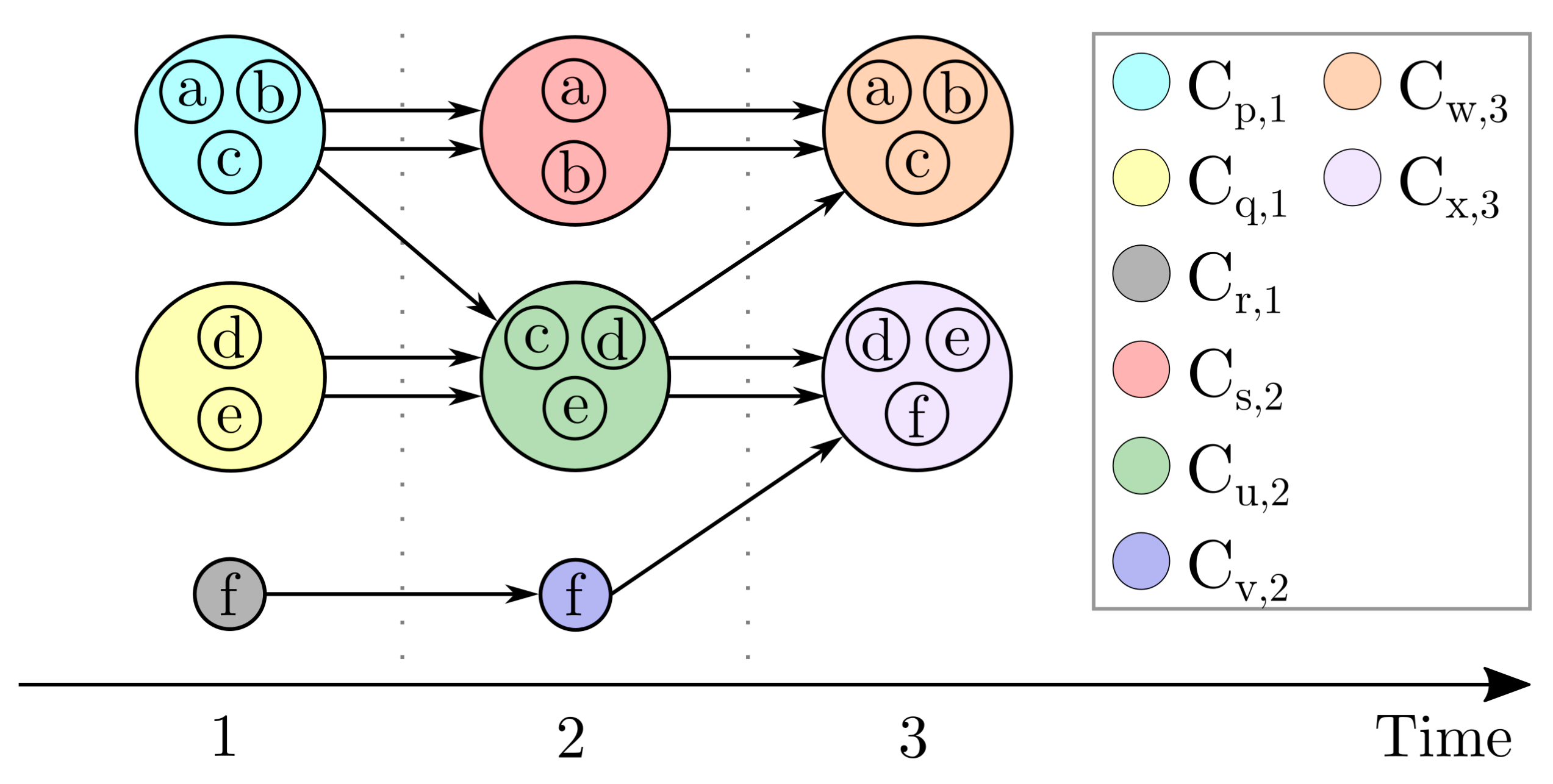
For a better illustration of the equations and corresponding calculations, we refer to the example given in Figure 1, which represents multiple time series clustered per timestamp. In the context of this work, data points defined as noise are considered as separate clusters. Thus, the data points of the time series $T{S}_f$ are assigned to the clusters $C_{r,1}$ and $C_{v,2}$ at timestamps one and two.

The first term which will be relevant in the rest of this section is the cluster transitions set $ct$. A single cluster transition of a time series $T{S}_y$ is a tuple of two cluster labels indicating in which clusters two adjacent data points of $T{S}_y$ are located. Thus, a set of cluster transitions $ct$ has the following definition:

$$ct\left(T{S}_y\right)=\{(C_{i,t},C_{j,t+1})\mid \exists y_t,y_{t+1}\in T{S}_y:y_t\in C_{i,t}\wedge y_{t+1}\in C_{i,t+1}\}.$$

(1)

For example, in Figure 1, the cluster transition sets of the time series $T{S}_c$ are:

$$ct\left(T{S}_c\right)=\{(C_{p,1},C_{u,2}),(C_{u,2},C_{w,3})\}.$$

Given the description of the cluster transition set, we next define a multiset M that contains all cluster transitions for all time series $T{S}_i$ of the data set D:

$$M_D=\bigcup _{T{S}_i\in D}ct\left(T{S}_i\right).$$

(2)

Regarding Figure 1, the multiset $M_D$ is:

$$\begin{array}{cc}\hfill M_D=& \left\{\right(C_{p,1},C_{s,2}),(C_{p,1},C_{s,2}),(C_{p,1},C_{u,2}),\hfill \\ & \hspace{0.17em}\hspace{0.17em}(C_{q,1},C_{u,2}),(C_{q,1},C_{u,2}),(C_{r,1},C_{v,2}),\hfill \\ & \hspace{0.17em}\hspace{0.17em}(C_{s,2},C_{w,3}),(C_{s,2},C_{w,3}),(C_{u,2},C_{w,3}),\hfill \\ & \hspace{0.17em}\hspace{0.17em}(C_{u,2},C_{x,3}),(C_{u,2},C_{x,3}),(C_{v,2},C_{x,3}){\}}_b.\hfill \end{array}$$

In combination with the equation for the cluster transition set, the given multiset description is then used to define a conformity score, which indicates how often a particular cluster transition p occurs in all time series of a data set D:

$$conformity\_score(p,M_D)=M_D\left(p\right).$$

(3)

With respect to this equation, the conformity score of the cluster transition $(C_{p,1},C_{s,2})$ of the data set D presented in Figure 1 is:

$$conformity\_score((C_{p,1},C_{s,2}),M_D)=M_D\left((C_{p,1},C_{s,2})\right)=2.$$

Using Equations (1)–(3), a set of anomalous transitions $at$ for a time series $T{S}_y\in D$ is defined as follows:

$$at\left(T{S}_y\right)=\{p\mid p\in ct\left(T{S}_y\right)\wedge conformity\_score(p,M_D)\le \sigma \},$$

(4)

where $\sigma$ is a threshold for the conformity score of a single cluster transition. Thus, if the conformity score is less than or equal to $\sigma$, then the corresponding transition is categorized as anomalous. Consequently, a subsequence $S_{y,[k,m]}$ of a time series $T{S}_y$ is anomalous if and only if:

$$at\left(S_{y,[k,m]}\right)=ct\left(S_{y,[k,m]}\right).$$

(5)

According to Equations (4) and (5), the entire time series $T{S}_c$ of the data set D shown in Figure 1 is anomalous due to:

$$at\left(T{S}_c\right)=\{(C_{p,1},C_{u,2}),(C_{u,2},C_{w,3})\}=ct\left(T{S}_c\right).$$

Using Equation (5), anomalous subsequences of a time series $T{S}_y$ can be identified by iterating over all possible subsequences of $T{S}_y$. As an alternative to this approach, a set of tuples can be derived based on the set of anomalous cluster transitions, where the first element of each tuple indicates the beginning of an anomalous subsequence, and the second one specifies the end of the corresponding subsequence. Given a lower number of required iterations through a time series, this alternative is intended to optimize the performance of the method presented in this paper. This first requires the definition of an order relation ≤:

$$(C_{i,t_a},C_{j,t_b})\le (C_{k,t_c},C_{l,t_d}):\iff (t_a\le t_b)\wedge (t_c\le t_d).$$

(6)

Based on the presented order relation, a set of tuples can be defined with respect to a time series $T{S}_y$, where each tuple consists of two anomalous cluster transitions. The first transition indicates the beginning of an anomalous subsequence of the time series $T{S}_y$, and the last one specifies the end of the corresponding subsequence. The formal description for this set of anomalous transition boundaries $atb$ is given by:

$$\begin{array}{cc}\hfill atb\left(T{S}_y\right)=\left\{\right(p,p^{\prime })& \mid (p,p^{\prime }\in at\left(T{S}_y\right))\wedge \hfill \\ & \hspace{0.17em}(\nexists \tilde{p}\in ct\left(T{S}_y\right)\wedge \tilde{p}\notin at\left(T{S}_y\right):p\le \tilde{p}\le p^{\prime })\wedge \hfill \\ & \hspace{0.17em}(\nexists (C_{i,t},C_{j,t+1})\in at\left(T{S}_y\right):p^{\prime }=(C_{h,t-1},C_{i,t}))\}.\hfill \end{array}$$

In the case of the time series $T{S}_c$ from Figure 1, the set of anomalous transition boundaries for $\sigma =1$ is:

$$atb\left(T{S}_c\right)=\left\{((C_{p,1},C_{u,2}),(C_{u,2},C_{w,3}))\right\}.$$

Further, to obtain data point-based outlier boundaries for a time series $T{S}_y$, a mapping $d{p}_y(C_{i,t},C_{j,t^{\prime }})=(y_t,y_t^{\prime })$ is required that maps cluster tuples to a tuple of data points based on $T{S}_y$, such that:

$$y_t\in T{S}_y\wedge y_t\in C_{i,t}\wedge y_{t^{\prime }}\in T{S}_y\wedge y_{t^{\prime }}\in C_{j,t^{\prime }}.$$

Finally, the outlier boundaries set $ob$ within a time series $T{S}_y$ is defined as a element-wise merge of tuples of the set of the anomalous transition boundaries, which is then mapped to the data points of $T{S}_y$:

$$ob\left(T{S}_y\right)=\left\{d{p}_y(C_{w,t},C_{z,t^{\prime }+1})\right|\forall ((C_{w,t},C_{x,t+1}),(C_{y,t^{\prime }},C_{z,t^{\prime }+1}))\in atb\left(T{S}_y\right)\}.$$

In this context, the set of outlier boundaries consists of tuples, where the first element of each tuple marks the beginning of an anomalous subsequence, and the second one indicates the end of that subsequence. Consequently, the outlier boundaries set of the time series $T{S}_c=c_1,c_2,c_3$ shown in Figure 1 for $\sigma =1$ is:

$$ob\left(T{S}_c\right)=\left\{d{p}_c(C_{p,1},C_{w,3})\right\}=\left\{(c_1,c_3)\right\}.$$

4. Experiments

In this section, we evaluate the method presented in this work. Since the method for detection of outliers in time series (DOOTS (https://github.com/tatusch/ots-eval/blob/main/doc/doots.md (accessed on 20 April 2022))) of Tatusch et al. [22] also detects anomalous subsequences based on time series transitions between different clusters, we used their method for comparison with our approach. In addition, we used the identical data sets and the same clustering method. This is intended to make the comparison of the two methods as fair as possible. In both approaches, DBSCAN with euclidean distance was used for timestamp-based clustering, with $minPts$ and $\epsilon$ set differently for each data set but equally for both methods. In order to identify the best cluster parameters, we made use of the cluster over-time stability evaluation measure called CLOSE [15] and found that these were the same as Tatusch et al. used in their study [16]. Furthermore, we used the same thresholds for DOOTS as proposed in Tatusch et al. In order to make a meaningful comparison with our method, we chose the conformity score threshold in a way to ensure the results of both methods were as similar as possible. Overall, we used two real world data sets to compare both methods.

4.1. Eikon Financial Data Set

One of the real world data sets Tatusch et al. used for the evaluation of their work was an extract from the EIKON database. This database contains financial data from over 150,000 sources worldwide, and the information includes the previous 65 years. The extract contained annual values from the features’ net sales and expected return for 30 (originally) random selected companies. The values of both features were normalized by min–max-normalization. The parameters used for the clustering by DBSCAN were $\epsilon =0.15$ and $minPts=2$.

Figure 2a shows the result of DOOTS [16] for the threshold $\tau =0.6$, and Figure 2b illustrates the result of our outlier detection method for the conformity score threshold of $\sigma =1$. The black dashed boxes in Figure 2a mark intuitive outliers, which by definition consist of noise, and the red boxes represent outliers found by analyzing cluster transitions (outlier by distance). In contrast, in Figure 2b, each black dashed box highlights the beginning of an anomalous subsequence and each red dashed box marks the remainder of that subsequence.

The most noticeable fact when comparing the results of both methods is the different number of detected subsequences. While DOOTS [16] found only two anomalous subsequences ($S_{GM,[2008,2009]}$ and $S_{KR,[2009,2013]}$), our solution identified four of them ($S_{GM,[2008,2009]}$, $S_{KR,[2008,2013]}$, $S_{TJX,[2008,2009]}$, and $S_{UPS,[2012,2013]}$). A detailed analysis of $S_{TJX,[2008,2009]}$ and $S_{UPS,[2012,2013]}$ showed that both of them had a unique cluster transition with a conformity score of one each. Since the threshold $\sigma$ was set to the same value, both subsequences were identified as anomalous by our method.

The explanation for why $S_{TJX,[2008,2009]}$ and $S_{UPS,[2012,2013]}$ were not considered anomalous by DOOTS [16] is more complex. In the case of UPS, neither a subsequence score nor the best score can be calculated, due to the lack of a cluster membership of the last data point of the time series. The inclusion of such a case requires an additional case differentiation. This can be seen as a disadvantage of the method of Tatusch et al. [16]. The reason for the missing detection of $S_{TJX,[2008,2009]}$ was the small size of the cluster in which TJX was located in 2008. Therefore, the calculation of the subsequence score for $S_{TJX,[2008,2009]}$ resulted in $0.5$. Since the best score for this subsequence was one, the outlier score for it was $(1-0.5)=1$, thus lower than the threshold $\tau$ of $0.6$. From this case, the dependence of the outlier detection result on the corresponding cluster sizes can be derived, which can be considered as another disadvantage of the method of DOOTS [16].

Most interesting with regard to the identification of UPS (2012–2013) and TJX (2008–2009) as outliers is probably the realization that they can be explained by related events. Unlike the companies with which UPS was clustered in 2012, UPS had to lower its expected return in 2013. This was probably attributable to the crash of UPS Airlines Flight 1354 (https://www.bbc.com/news/world-us-canada-23698279; accessed on 25 April 2022) 14 August 2013. TJX Companies is a multinational department store corporation that in 2009 was still struggling with the consequences of the recession triggered by the economic crisis in 2008 (https://www.bizjournals.com/denver/stories/2009/07/06/daily63.html; accessed on 25 April 2022). For this reason, sales fell sharply, as they did for all retail traders. The reason why TJX was identified as an outlier here was that it was the only retail company in the data set.

4.2. Airline On-Time Performance Data Set

The other real world data set that Tatusch et al. [16] used in their publication was called “Airline on-time performance”. It was originally created for a challenge with the goal to predict delayed and canceled flights. Therefore, the authors included flight data on all commercial flights in the USA between October 1987 and April 2008, resulting in a total of 120 million records. Based on this data set, Tatusch et al. [16] generated one dimensional time series with the feature “distance”. As described in their work, they took eight days of every month and calculated the average distance for each airline in the data set. Before the authors clustered the created data set with DBSCAN, they normalized the distances by the min–max normalization. The parameters for the applied clustering algorithm were $minPts=3$ and $ϵ=0.03$.

The result of DOOTS [16] for $\tau =0.4$ is displayed in Figure 3a. Here, the black solid lines represent outliers by distance, and the black dashed lines are both outliers by distance and intuitive outliers. Our result for $\sigma =1$ is shown in Figure 3b, where the black solid lines mark anomalous subsequences. In both figures, the colors of the dots set at each time point represent the cluster membership, with the red color representing noise found by DBSCAN. The results of both methods show strong similarities regarding the detection of anomalous subsequences, but there are also some differences. The most relevant of them are discussed below.

Foremost, the subsequences $S_{A,[1,2]}$ and $S_{A,[3,4]}$ of the time series marked as A in Figure 3 were detected as anomalous by DOOTS [16], while they were not detected as such by our method. In the context of our approach, these subsequences were not detected as anomalous, because the number of equal cluster transitions and, therefore, the conformity score of $S_{A,[1,2]}$ as well as of $S_{A,[3,4]}$ was higher than the threshold $\sigma =1$. In contrast, explaining the results of DOOTS [16] requires detailed calculations. First, the subsequence score for $S_{A,[1,2]}$ is:

$$subseq\_score\left(S_{A,[1,2]}\right)=3/4=0.75.$$

Given that the best score for the last cluster of $S_{A,[1,2]}$ is one, the outlier score for this subsequence is:

$$outlier\_score\left(S_{A,[1,2]}\right)=1-0.75=0.25<\tau .$$

Based on this result, $S_{A,[1,2]}$ should not be labeled as anomalous. However, if we take the subsequence $S_{A,[1,3]}$, which in addition to $S_{A,[1,2]}$ contains a further value at $time=3$, the subsequence score for $S_{A,[1,3]}$ becomes smaller compared to $S_{A,[1,2]}$ with:

$$subseq\_score\left(S_{A,[1,3]}\right)=0.5\ast (0.5+0.1)=0.3.$$

Since the best score for the corresponding cluster at $time=3$ is one, the outlier score for $S_{A,[1,3]}$ is:

$$outlier\_score\left(S_{A,[1,3]}\right)=1-0.3=0.7>\tau .$$

Thus, the subsequence $S_{A,[1,3]}$, was marked as anomalous. The same type of calculations led to the detection of the subsequence $S_{A,[3,5]}$ as anomalous, which contained the not anomalous subsequence $S_{A,[3,4]}$.

The detection of $S_{A,[1,2]}$ and $S_{A,[3,4]}$ by DOOTS [16] leads to two possible conclusions. On one hand, it can be concluded that the approach of Tatusch et al. [16] considers anomalous subsequences in a broader context with respect to the length of a time series than our method, which would be an advantage of DOOTS. On the other hand, this solution leads to subsequences that are not anomalous within their interval being detected as anomalous. This can be seen as a disadvantage of DOOTS [16]. In contrast, our method detects only those subsequences that exhibit suspicious behavior within their time interval. However, a broader context regarding our detection method can be achieved by additionally considering non-anomalous subsequences that are adjacent to detected anomalous subsequences.

A more general observation is that our method detected every subsequence of length two as anomalous if it contained one or more noisy data points. The reason for this is that the conformity score of such sequences was one and thus smaller or equal to the chosen threshold $\sigma$. In contrast, the solution of Tatusch et al. [16] follows a different approach. Even if a subsequence of length two had a noisy data point, it does not mean that DOOTS [16] would detect this subsequence as anomalous. In addition to the subsequence score, the detection of outliers by the method of Tatusch et al. [16] also depends on the value of the corresponding best score and whether both scores can be calculated for the given subsequence. In summary, we can conclude that DOOTS [16] has a much more complex set of rules than our method, whereby the results of both methods are similar.

5. Conclusions and Future Work

In this paper, we introduced a new approach for detecting outliers in multiple multivariate time series. For this purpose, we first clustered the time series data at each time point and then calculated conformity scores for each subsequence of length two. Finally, we determined whether the conformity scores were less than or equal to the specified threshold and labeled them as outliers if they were.

Since we found only one alternative algorithm (called DOOTS) [16] based on a similar idea, we compared the two in detail. The application of both methods led to similar results, although our solution had a much simpler rule set and, therefore, required fewer calculations (the runtime estimation is provided in Section 2). On one hand, this simplified the understanding of the origin of the outliers and, on the other hand, the better performance of our method allows it to be used on real time data. In addition, our rule set seems to be more consistent in contrast to DOOTS [16]. This statement is supported, among other things, by comparing the thresholds of both methods. While for our method the same minimum conformity score threshold was used in each dataset, the threshold set in DOOTS [16] varied without much difference between the results of both methods. Furthermore, our solution detected subsequences even if they ended with a noisy data point.

The most important drawback of our method is that the outlier detection result depends highly on the result of previous clustering. This implies that a poor clustering result would lead to a poor detection result of our method. Since the analysis of cluster transitions is the core idea of our method, we have to rely on approaches such as CLOSE [15] to obtain reasonable clustering results for our solution. Furthermore, while our method can be applied to real-time data due to its performance, this requires prior clustering in real-time with reasonable results for time series data. Here, CLOSE [15] provides good results, but the procedure is not applicable to real-time data because of the high number of needed computations. Given that, the most important aspect for future work is to optimize CLOSE [15] for real-time application. In addition, the freely selectable threshold $\sigma$ in our work has a high impact on the detection result of our method. Every increment of $\sigma$ leads to a superset of detected outliers regarding the result of the previous threshold. Although in this work we set this parameter to one for each dataset in order to obtain results that were as similar as possible and thus comparable to DOOTS [16], the optimal value for $\sigma$ can be determined in several ways, and each determination should depend on the dataset in question. One way to determine the optimal $\sigma$ is to count the cluster transitions that occur, sort them in ascending order, and choose the value for $\sigma$ at which the slope change is greatest. However, the analysis of this and other possible methods is beyond the scope of this work and should therefore be addressed in future work. Another aspect is that not all detected anomalous subsequences may be useful in the context of given requirements. Since this case requires further analysis, our method could be applied to multiple data sets in which the outliers have already been labeled.