Expectation-Maximization Algorithm for Autoregressive Models with Cauchy Innovations ^†

Abstract

In this paper, we study the autoregressive (AR) models with Cauchy distributed innovations. In the AR models, the response variable $y_t$ depends on previous terms and a stochastic term (the innovation). In the classical version, the AR models are based on normal distribution which could not capture the extreme values or asymmetric behavior of data. In this work, we consider the AR model with Cauchy innovations, which is a heavy-tailed distribution. We derive closed forms for the estimates of parameters of the considered model using the expectation-maximization (EM) algorithm. The efficacy of the estimation procedure is shown on the simulated data. The comparison of the proposed EM algorithm is shown with the maximum likelihood (ML) estimation method. Moreover, we also discuss the joint characteristic function of the AR(1) model with Cauchy innovations, which can also be used to estimate the parameters of the model using empirical characteristic function.

1. Introduction

Autoregressive (AR) models with stable and heavy-tailed innovations are of great interest in time series modeling. These distributions can easily assimilate the asymmetry, skewness, and outliers present in time series data. The Cauchy distribution is a special case of stable distribution with undefined expected value, variance, and higher order moments. The Cauchy distribution and its mixture has many applications in the field of economics [1], seismology [2], biology [3], and various other fields, but only a few studies have been conducted concerning time series models with Cauchy errors. In [4], the maximum likelihood (ML) estimation of AR(1) model with Cauchy errors is studied.

The standard estimation techniques for the AR(p) model with Cauchy innovations, particularly the Yule–Walker method and conditional least squares method, cannot be used due to the infinite second order moments of the Cauchy distribution. Therefore, it is worthwhile to study and assess the alternate estimation techniques for the AR(p) model with Cauchy innovations. In the literature, several estimation techniques have been proposed to estimate the parameters of AR models with infinite variance errors (see e.g., [5,6,7]).

In this paper, we propose to use the EM algorithm to estimate the parameters of the distribution and model simultaneously. It is a general iterative algorithm for model parameter estimation which iterates between two steps, namely the expectation step (E-step) and the maximization step (M-step) [8]. It is an alternative to the numerical optimization of the likelihood function which is proven to be numerically stable [9]. We also provide the formula based on the characteristic function (CF) and empirical characteristic function (ECF) of Cauchy distribution for AR(p) model estimation. The idea to use ECF in a time series stable ARMA model has been discussed in [10].

The remainder of the paper is organized as follows. In Section 2, we present a brief overview of the Cauchy AR(p) model, followed by a discussion of estimation techniques, namely the EM algorithm and estimation by CF and ECF. Section 3 checks the efficacy of the estimation procedure on simulated data. We also present the comparative study, where the proposed technique is compared with ML estimation for Cauchy innovations. Section 4 concludes the paper.

2. Cauchy Autoregressive Model

We consider the AR(p) univariate stationary time-series $\left\{Y_t\right\}$, $t\in \mathbb{N}$ with Cauchy innovations defined as

$$\begin{array}{c}\hfill Y_t=\sum _{i=1}^p{\rho }_i{Y}_{t-i}+{\epsilon }_t={\rho }^T{Y}_{t-1}+{\epsilon }_t,\end{array}$$

(1)

where $\rho ={({\rho }_1,{\rho }_2,\cdots ,{\rho }_p)}^T$ is a p-dimensional column vector, $Y_{t-1}={(Y_{t-1},Y_{t-2},\cdots ,Y_{t-p})}^T$ is a vector of p lag terms, and $\left\{{ϵ}_t\right\}$, $t\in \mathbb{N}$ are i.i.d. innovations distributed as Cauchy$(\alpha ,\gamma )$. The pdf of Cauchy$(\alpha ,\gamma )$ [11] is

$$\begin{array}{c}\hfill f(x;\alpha ,\gamma )=\frac{\gamma }{\pi }\left[\frac{1}{{\gamma }^2+{(x-\alpha )}^2}\right],\gamma >0,\alpha \in \mathbb{R},x\in \mathbb{R}.\end{array}$$

(2)

The conditional distribution of $Y_t$ given the preceding data ${\mathcal{F}}_{t-1}={(Y_{t-1},Y_{t-2},\cdots ,Y_1)}^T$ is given by [4]

$$\begin{array}{cc}\hfill p\left(Y_t\right|{\mathcal{F}}_{t-1})& =f(y_t-{\rho }^T{y}_{t-1};\alpha ,\gamma )=\frac{\gamma }{\pi }\left[\frac{1}{{\gamma }^2+{(y_t-{\rho }^T{y}_{t-1}-\alpha )}^2}\right],\hfill \end{array}$$

where $y_{t-1}$ is the realization of $Y_{t-1}$. In the next subsection, we propose the methods to estimate the model parameters $\rho$ and innovation parameters $\alpha$ and $\gamma$ simultaneously.

2.1. Parameter Estimation Using EM Algorithm

We estimate the parameters of the AR(p) model using an EM algorithm which maximizes the likelihood function iteratively. Further, we discuss the time series $\left\{Y_t\right\}$ using the characteristic function (CF) and estimation method using CF and ECF. Recently [7], the exponential-squared estimator for AR models with heavy-tailed errors was introduced and proven to be $\sqrt{n}$-consistent under some regularity conditions; similarly, the self-weighted least absolute deviation estimation method was also studied for the infinite variance AR model [12]. The ML estimation of AR models with Cauchy errors with intercept and with linear trend is studied, and the AR coefficient is shown to be $n^{3/2}$-consistent under some conditions [4]. For the AR(p) model with Cauchy innovations with n samples, the log likelihood is defined as

$$\begin{array}{cc}\hfill l(\Theta )& =(n-p)log\left(\gamma \right)-(n-p)log\left(\pi \right)-\sum _{t=p+1}^{n}log({\gamma }^2+{(y_t-{\rho }^T{Y}_{t-1}-\alpha )}^2),\hfill \end{array}$$

where $\Theta =\left(\alpha ,\gamma ,{\rho }^T\right).$

Proposition 1.

Consider the AR(p) time-series model given in Equation (1) where error terms follow Cauchy$(\alpha ,\gamma )$. The maximum likelihood estimates of the model parameters using EM algorithm are as follows

$$\begin{array}{c}\hfill \begin{array}{cc}\hfill {\widehat{\rho }}^T& =\left(\sum _{t=p+1}^n\frac{(y_t-\alpha )Y_{t-1}^T}{s_t^{\left(k\right)}}\right){\left({\displaystyle \sum _{t=p+1}^n\frac{Y_{t-1}{Y}_{t-1}^T}{s_t^{\left(k\right)}}}\right)}^{-1};\hfill \\ \hfill \widehat{\alpha }& =\frac{{\displaystyle \sum _{t=p+1}^n\frac{(y_t-{\rho }^T{Y}_{t-1})}{s_t^{\left(k\right)}}}}{{\sum }_{t=p+1}^n\frac{1}{s_t^{\left(k\right)}}};\hfill \\ \hfill & and\hfill \\ \hfill \widehat{\gamma }& =\sqrt{\frac{n-p}{2{\sum }_{t=p+1}^n\frac{1}{s_t^{\left(k\right)}}}},\hfill \end{array}\end{array}$$

(3)

where $s_t^{\left(k\right)}={(y_t-{{\rho }^T}^{\left(k\right)}{Y}_{t-1}-{\alpha }^{\left(k\right)})}^2+{{\gamma }^{\left(k\right)}}^2$.

Proof. 

Consider the AR(p) model

$$Y_t={\rho }^T{Y}_{t-1}+{\epsilon }_t,t=p+1,2,\cdots ,n,$$

where ${\epsilon }_t$ follows Cauchy distribution Cauchy$(\alpha ,\gamma )$. Let $({\epsilon }_t,V_t)$ for $t=1,2,\cdots ,n$ denote the complete data for innovations $\epsilon$. The observed data ${\epsilon }_t$ are assumed to be from Cauchy$(\alpha ,\gamma )$ and the unobserved data $V_t$ follow inverse gamma IG$(1/2,{\gamma }^2/2)$. A random variable V∼IG$(a,b)$ if the pdf is given by

$$f_V(v;a,b)=\frac{b^a}{\Gamma \left(a\right)}\frac{e^{-b/v}}{v^{a+1}},a>0,b>0,v>0.$$

We can rewrite ${\epsilon }_t$ as ${\epsilon }_t=Y_t-{\rho }^T{Y}_{t-1},\mathrm{for}t=1,2,\cdots ,n.$ The stochastic relation $\epsilon =\alpha +\sqrt{V}Z$ with $Z\sim N(0,1)$ i.e., standard normal and $V\sim \mathrm{IG}(1/2,{\gamma }^2/2)$ is used to generate Cauchy$(\alpha ,\gamma )$ distribution. Then, the conditional distribution is

$$\begin{array}{c}\hfill f(\epsilon ={ϵ}_t|V=v_t)=\frac{1}{\sqrt{2\pi v_t}}exp\left(-\frac{1}{2v_t}({ϵ}_t-\alpha ){)}^2\right).\end{array}$$

Now, we need to estimate the unknown parameters $\Theta =(\alpha ,\gamma ,{\rho }^T)$. To apply the EM algorithm for estimation, we first find the conditional expectation of log-likelihood of complete data $(\epsilon ,V)$ with respect to the conditional distribution of V given $\epsilon$. As the unobserved data are assumed to be from IG$(1/2,{\gamma }^2/2)$, the posterior distribution is again an inverse gamma i.e.,

$$V|\epsilon =e,\Theta \sim \mathrm{IG}\left(1,\frac{{(e-\alpha )}^2+{\gamma }^2}{2}\right).$$

The following conditional inverse first moment and $\mathbb{E}(log(V\left)\right|\epsilon =e)$ will be used in calculating the conditional expectation of the log-likelihood function:

$$\begin{array}{cc}\hfill \mathbb{E}\left(V^{-1}\right|\epsilon =e)& =\frac{2}{{(e-\alpha )}^2+{\gamma }^2},\hfill \\ \hfill \mathbb{E}(log(V\left)\right|\epsilon =e)& =log({(e-\alpha )}^2+{\gamma }^2)-log2+0.5776.\hfill \end{array}$$

The complete data likelihood is given by

$$\begin{array}{cc}\hfill L(\Theta )& =\prod _{t=p+1}^{n}f({ϵ}_t,v_t)=\prod _{t=p+1}^n{f}_{\epsilon |V}\left({ϵ}_t\right|v_t)f_V\left(v_t\right)\hfill \\ \hfill & =\prod _{t=p+1}^n\frac{\gamma }{2\pi v_t^2}exp\left(-\frac{{({ϵ}_t-\alpha )}^2+{\gamma }^2}{2v_t}\right).\hfill \end{array}$$

The log likelihood function will be

$$\begin{array}{cc}\hfill l(\Theta )& =(n-p)log\left(\gamma \right)-(n-p)log\left(2\pi \right)-2\sum _{t=p+1}^{n}log\left(v_t\right)-\sum _{t=p+1}^n\frac{{({ϵ}_t-\alpha )}^2+{\gamma }^2}{2v_t}.\hfill \end{array}$$

Now, we will use the relation ${ϵ}_t=Y_t-{\rho }^T{Y}_{t-1}$ in further calculations. In the first step at kth iteration, E-step of EM algorithm, we need to compute the expected value of the complete data log likelihood known as $Q(\Theta |{\Theta }^{\left(k\right)})$, which is expressed as

$$\begin{array}{cc}\hfill Q(\Theta |{\Theta }^{\left(k\right)})& ={\mathbb{E}}_{V|\epsilon ,{\Theta }^{\left(k\right)}}[logf(\epsilon ,V|\Theta )|{ϵ}_t,{\Theta }^{\left(k\right)}]={\mathbb{E}}_{V|\epsilon ,{\Theta }^{\left(k\right)}}\left[l(\Theta |{\Theta }^{\left(k\right)})\right]\hfill \\ \hfill & =(n-p)log\gamma -(n-p)log2\pi -\sum _{t=p+1}^n\mathbb{E}(log{v}_t|{ϵ}_t,{\Theta }^{\left(k\right)})\hfill \\ \hfill & -\frac{{\gamma }^2}{2}\sum _{t=p+1}^n\mathbb{E}\left(v_t^{-1}\right|{ϵ}_t,{\Theta }^{\left(k\right)})-\frac{1}{2}\sum _{t=p+1}^n{({ϵ}_t-\alpha )}^2\mathbb{E}\left(v_t^{-1}\right|{ϵ}_t,{\Theta }^{\left(k\right)})\hfill \\ \hfill & =(n-p)log\gamma -(n-p)log2\pi -(n-p)log2+0.5776(n-p)-\sum _{t=p+1}^{n}log({({ϵ}_t-{\alpha }^{\left(k\right)})}^2+{{\gamma }^{\left(k\right)}}^2)\hfill \\ \hfill & -\frac{{\gamma }^2}{2}\sum _{t=p+1}^n\frac{1}{{({ϵ}_t-{\alpha }^{\left(k\right)})}^2+{{\gamma }^{\left(k\right)}}^2}-\sum _{t=p+1}^n\frac{{({ϵ}_t-\alpha )}^2}{{({ϵ}_t-{\alpha }^{\left(k\right)})}^2+{{\gamma }^{\left(k\right)}}^2}\hfill \\ \hfill & =(n-p)log\gamma -(n-p)log2\pi -(n-p)log2+0.5776(n-p)-\sum _{t=p+1}^{n}log\left(s_t^{\left(k\right)}\right)\hfill \\ \hfill & -\frac{{\gamma }^2}{2}\sum _{t=p+1}^n\frac{1}{s_t^{\left(k\right)}}-\sum _{t=p+1}^n\frac{{({ϵ}_t-\alpha )}^2}{s_t^{\left(k\right)}}.\hfill \end{array}$$

where $s_t={(y_t-{\rho }^T{Y}_{t-1}-\alpha )}^2+{\gamma }^2$. In the next M-step, we estimate the parameters $\alpha ,\gamma ,\mathrm{and}{\rho }^T$ by maximizing the Q function using the equations below:

$$\begin{array}{cc}\hfill \frac{\partial Q}{\partial \rho }& =4\sum _{t=p+1}^n\frac{(y_t-{\rho }^T{Y}_{t-1}-\alpha Y_{t-1}^T)}{s_t^{\left(k\right)}},\hfill \\ \hfill \frac{\partial Q}{\partial \alpha }& =\sum _{t=p+1}^n\frac{(y_t-{\rho }^T{Y}_{t-1}-\alpha )}{s_t^{\left(k\right)}},\hfill \\ \hfill \frac{\partial Q}{\partial \gamma }& =\frac{n-p}{\gamma }-2\gamma \sum _{t=p+1}^n\frac{1}{s_t^{\left(k\right)}}.\hfill \end{array}$$

Solving the above equations at each iteration, we find the following closed form estimates of the parameters at $k+1$th iteration:

$$\begin{array}{c}\hfill \begin{array}{cc}\hfill {\widehat{\rho }}^T& =\left(\sum _{t=p+1}^n\frac{(y_t-\alpha )Y_{t-1}^T}{s_t^{\left(k\right)}}\right){\left({\displaystyle \sum _{t=p+1}^n\frac{Y_{t-1}{Y}_{t-1}^T}{s_t^{\left(k\right)}}}\right)}^{-1};\hfill \\ \hfill \widehat{\alpha }& =\frac{{\displaystyle \sum _{t=p+1}^n\frac{(y_t-{\rho }^T{Y}_{t-1})}{s_t^{\left(k\right)}}}}{{\sum }_{t=p+1}^n\frac{1}{s_t^{\left(k\right)}}};\hfill \\ \hfill & and\hfill \\ \hfill \widehat{\gamma }& =\sqrt{\frac{n-p}{2{\sum }_{t=p+1}^n\frac{1}{s_t^{\left(k\right)}}}},\hfill \end{array}\end{array}$$

(4)

where $s_t^{\left(k\right)}={(y_t-{{\rho }^T}^{\left(k\right)}{Y}_{t-1}-{\alpha }^{\left(k\right)})}^2+{{\gamma }^{\left(k\right)}}^2$. □

2.2. Characteristic Function for Estimation

Thus far, we have considered the conditional distribution of $Y_t$ given the preceding data ${\mathcal{F}}_{t-1}$. Now, we include the dependency of time series $\left\{Y_t\right\}$ by defining the variable $d_j=(y_j,\cdots ,y_{j+p})$ for $j=1,\cdots ,n-p.$ In each variable $\left\{d_j\right\}$, there are p terms the same as adjacent variable. The distribution of $\left\{d_j\right\}$ will be multivariate Cauchy with dimension $r=p+1$.

The CF of each $d_j$ is $c(\Theta ,s)=\mathbb{E}(exp\left(i{s}^T{d}_j\right))$ and the ECF is $c_n\left(s\right)=\frac{1}{n}{\sum }_{j=1}^{n-p}exp\left(i{s}^T{d}_j\right)$ where $s={(s_1,\cdots ,s_{p+1})}^T.$

To estimate the parameters using CF and ECF, we make sure that the joint CF of the AR(p) model has a closed form. In the next result, the closed form expression for the joint CF of the AR(1) model with Cauchy innovations is given.

Proposition 2.

The joint CF of stationary AR(1) model with Cauchy innovations is

$$c(s_1,s_2;\Theta )=exp\left[i\alpha (s_1+s_2)\left(\frac{1}{1-\rho }\right)\right]\times exp\left[-\gamma \left(|s_2|+|s_1+\rho s_2|\left(\frac{1}{1-\left|\rho \right|}\right)\right)\right].$$

Proof. 

For stationary AR(1) model $y_t=\rho y_{t-1}+{\epsilon }_t$, we can rewrite it as

$$y_t={\epsilon }_t+\rho {\epsilon }_{t-1}+{\rho }^2{\epsilon }_{t-2}+{\rho }^3{\epsilon }_{t-3}+\cdots .$$

Note that $\left\{{\epsilon }_t\right\}$ are i.i.d from Cauchy$(\alpha ,\gamma )$ distribution, and the CF of Cauchy$(\alpha ,\gamma )$ is $\mathbb{E}(exp\left(is{\epsilon }_t\right))=exp(i\alpha s-\gamma |s\left|\right)$ [11]. Then, the joint CF of $(y_t,y_{t-1})$ is calculated as follows:

$$\begin{array}{cc}\hfill c(s_1,s_2;\Theta )& =\mathbb{E}[exp(i{s}_1{y}_{t-1}+i{s}_2{y}_t)]\hfill \\ \hfill & =\mathbb{E}[exp\left(i{s}_1({\epsilon }_{t-1}+\rho {\epsilon }_{t-2}+{\rho }^2{\epsilon }_{t-3}+\cdots )\right)+i{s}_2({\epsilon }_t+\rho {\epsilon }_{t-1}+{\rho }^2{\epsilon }_{t-2}+\cdots )]\hfill \\ \hfill & =\mathbb{E}[exp(i{s}_2{\epsilon }_t+i(s_1+s_2\rho ){\epsilon }_{t-1}+i\rho (s_1+\rho s_2){\epsilon }_{t-2}+\cdots )]\hfill \\ \hfill & =exp(i\alpha s_2-\gamma |s_2\left|\right)\times exp(i\alpha (s_1+\rho s_2)-\gamma |s_1+\rho s_2\left|\right)\hfill \\ \hfill & \times exp(i\alpha (\rho s_1+{\rho }^2{s}_2)-\gamma |\rho s_1+{\rho }^2{s}_2\left|\right)\times \cdots .\hfill \\ \hfill & =exp\left(i\alpha (s_1+s_2)(1+\rho +{\rho }^2+{\rho }^3+\cdots )\right)\hfill \\ \hfill & \times exp(-\gamma (|s_2|+|s_1+\rho s_2|+|\rho \left|\right|s_1+\rho s_2|+|{\rho }^2\left|\right|s_1+\rho s_2|+\cdots ))\hfill \\ \hfill & =exp(i\alpha (s_1+s_2)\left(\frac{1}{1-\rho }\right)\times exp(-\gamma (|s_2|+|s_1+\rho s_2\left|\right(1+\left|\rho \right|+|{\rho }^2|+\cdots )\left)\right)\hfill \\ \hfill & =exp\left[i\alpha (s_1+s_2)\left(\frac{1}{1-\rho }\right)\right]\times exp\left[-\gamma \left(|s_2|+|s_1+\rho s_2|\left(\frac{1}{1-\left|\rho \right|}\right)\right)\right].\hfill \end{array}$$

□

The joint CF for a higher dimension can be obtained in similar manner. Now, the model parameters can be estimated by solving the following integral with CF and ECF as defined in [10]:

$$\begin{array}{c}\hfill \int \dots \int w_{\Theta }\left(\mathit{s}\right)(c_n\left(\mathit{s}\right)-c(\mathit{s};\Theta ))d\mathit{s}=0.\end{array}$$

(5)

where optimal weight function

$$\begin{array}{c}\hfill w_{\Theta }^{\ast }\left(\mathit{s}\right)=\frac{1}{2\pi }\int \dots \int exp(-i{\mathit{s}}^{\mathit{T}}{\mathit{d}}_{\mathit{j}})\frac{\partial logf\left(y_{j+p}\right|y_j,\cdots ,y_{j+p-1})}{\partial \Theta }d{y}_j\cdots d{y}_{j+p}.\end{array}$$

(6)

Remark 1.

For a stationary AR(l) process $\left\{Y_t\right\}$ with $p=l$, the ECF estimator defined by Equation (5) with optimal weight function defined in Equation (6) is a conditional ML (CML) estimator and hence asymptotically efficient. The conditional log pdf for Cauchy distribution is:

$$logf\left(y_{j+p}\right|y_j,\cdots ,y_{j+p-1})=log\gamma -log\pi -log\left({\gamma }^2+{(y_t-{\rho }^T{Y}_{t-1}-{\alpha }^2)}^2\right).$$

The proof is similar to the proof of Proposition $2.1$ in [10].

3. Simulation Study

In this section, we assess the proposed model and the introduced estimation technique using a simulated data set. We discuss the estimation procedure for the AR(2) model with Cauchy innovations. The AR$\left(2\right)$ model defined in (1) is simulated with ${\rho }_1$ and ${\rho }_2$ as model parameters. We generate 1000 trajectories, each of size $N=500$ of Cauchy innovations using the normal variance-mean mixture form $\epsilon =\alpha +\sqrt{V}Z$ with $Z\sim N(0,1)$, i.e., standard normal and $V\sim \mathrm{IG}(1/2,{\gamma }^2/2).$ We then use the following simulation steps to generate the Cauchy innovations:

• step 1: Generate standard normal variate Z;
• step 2: Generate inverse gamma random variate IG$(1/2,{\gamma }^2/2)$ with $\gamma =2$;
• step 3: Using the relation $\epsilon =\alpha +\sqrt{V}Z$, we simulate the Cauchy innovations with $\alpha =1$;
• step 4: The time series data $y_t$ is generated with model parameters ${\rho }_1=0.5$ and ${\rho }_2=0.3.$

The exemplary time series data plot and scatter plot of innovation terms are shown in Figure 1. We apply the discussed EM algorithm to estimate the model parameters and distribution parameters. The relative change in the parameters is considered to terminate the algorithm. The following is the stopping criteria which is commonly used in literature:

$$max\left\{\left|\frac{{\alpha }^{(k+1)}-{\alpha }^{\left(k\right)}}{{\alpha }^{\left(k\right)}}\right|,\left|\frac{{\gamma }^{(k+1)}-{\gamma }^{\left(k\right)}}{{\gamma }^{\left(k\right)}}\right|,\left|\frac{{\rho }_1^{(k+1)}-{\rho }_1^{\left(k\right)}}{{\rho }_1^{\left(k\right)}}\right|,\left|\frac{{\rho }_2^{(k+1)}-{\rho }_2^{\left(k\right)}}{{\rho }_2^{\left(k\right)}}\right|\right\}<{10}^{-4}.$$

(7)

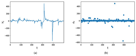
Figure 1. (a) The data plot of exemplary time series of length $N=500$ and (b) the scatter plot of the corresponding innovation terms of the AR(2) model with Cauchy innovations. The chosen parameters of the model are ${\rho }_1=0.5,{\rho }_2=0.3,\alpha =1,$ and $\gamma =2$.

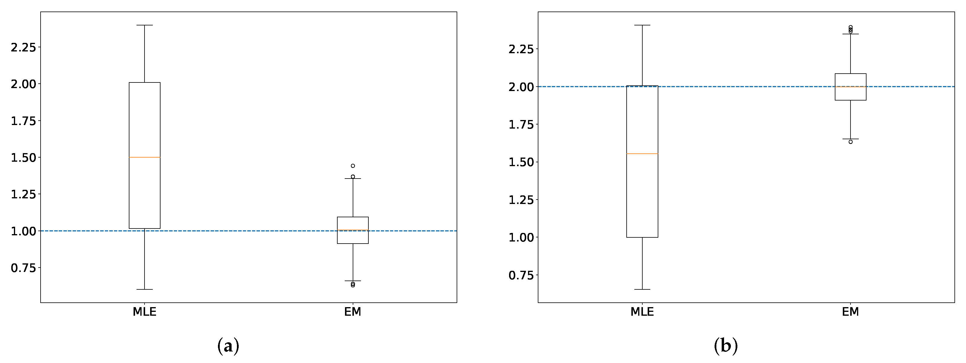
We compare the estimation results of Cauchy$(\alpha ,\gamma )$ with the EM algorithm and maximum likelihood (ML) estimation. The ML estimates are computed using the inbuilt function “mlcauchy” in R, which uses the exponential transform of the location parameter and performs non-linear minimization by a Newton-type algorithm. The comparison of the estimates of Cauchy($\alpha ,\gamma$) are shown in boxplots in Figure 2. From the boxplots, we find that the EM algorithm converges near to the true value of the Cauchy$(\alpha ,\gamma )$ as compared to the ML estimation. There is a possibility of achieving a better result from ML method if a different algorithm or inbuilt function for optimization are used for estimation.

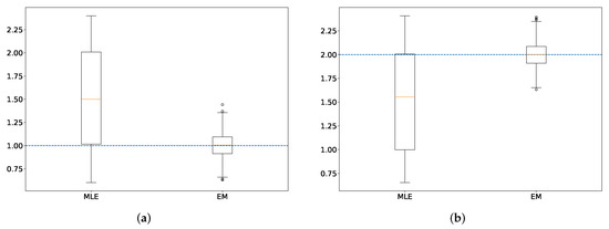
Figure 2. Boxplots of the estimates of the AR(2) model’s parameters with theoretical values (a) $\alpha =1$ and (b) $\gamma =2$ represented with blue dotted lines. The boxplots are created using 1000 trajectories, each of length 500.

4. Conclusions and Future Scope

In this work, we derive the closed form of estimates of AR model with Cauchy innovations using an EM algorithm. The performance of the proposed algorithm is compared with the ML method using simulated data. The ML estimation is found using an inbuilt function in R. Another benefit of using the EM algorithm is that it calculates the model as well as the innovation parameters simultaneously. It is evident from the boxplot that the EM algorithm outperforms the ML method. Further, we discuss another approach based on CF to estimate the AR model parameters with stable distribution. In the future, we plan to study and compare the proposed algorithm and ECF based estimation method with the existing techniques in [5,6,7] for an AR model with infinite variance. Further, the real life phenomena can be studied using the proposed model and methods.

References

- Liu, T.; Zhang, P.; Dai, W.S.; Xie, M. An intermediate distribution between Gaussian and Cauchy distributions. Phys. A Stat. Mech. Appl. 2012, 391, 5411–5421. [Google Scholar] [CrossRef] [Green Version]
- Kagan, Y.Y. Correlations of earthquake focal mechanism. Geophys. J. Int. 1992, 110, 305–320. [Google Scholar] [CrossRef] [Green Version]
- Bjerkedal, T. Acquisition of resistance in guinea pigs infected with different doses of virulent tubercle bacilli. Am. J. Hyg. 1960, 72, 130–148. [Google Scholar] [PubMed]
- Choi, J.; Choi, I. Maximum likelihood estimation of autoregressive models with a near unit root and Cauchy errors. Ann. Inst. Stat. Math. 2019, 71, 1121–1142. [Google Scholar] [CrossRef]
- Jiang, Y. An exponential-squared estimator in the autoregressive model with heavy-tailed errors. Stat. Interface 2016, 9, 233–238. [Google Scholar] [CrossRef]
- Li, J.; Liang, W.; He, S.; Wu, X. Empirical likelihood for the smoothed LAD estimator in infinite variance autoregressive models. Statist. Probab. Lett. 2010, 80, 1420–1430. [Google Scholar] [CrossRef]
- Tang, L.; Zhou, Z.; Wu, C. Efficient estimation and variable selection for infinite variance autoregressive models. J. Appl. Math. Comput. 2012, 40, 399–413. [Google Scholar] [CrossRef]
- Dempster, A.P.; Laird, N.M.; Rubin, D.B. Maximum likelihood from incomplete data via EM Algorithm. J. R. Stat. Soc. Ser. B 1977, 39, 1–22. [Google Scholar]
- McLachlan, G.J.; Krishnan, T. The EM Algorithm and Extensions, 2nd ed.; John Wiley & Sons: Hoboken, NJ, USA, 2007. [Google Scholar]
- Yu, J.; Knight, J.L. Empirical characteristic function in time series estimation. Econom. Theory 2002, 18, 691–721. [Google Scholar]
- Feller, W. An Introduction to Probability Theory and Its Applications, 2nd ed.; John Wiley & Sons: New York, NY, USA, 1991; Volume 2. [Google Scholar]
- Ling, S. Self-weighted least absolute deviation estimation for infinite variance autoregressive models. J. R. Stat. Soc. Ser. B 2005, 67, 381–393. [Google Scholar] [CrossRef]
Publisher’s Note: MDPI stays neutral with regard to jurisdictional claims in published maps and institutional affiliations. |
© 2022 by the authors. Licensee MDPI, Basel, Switzerland. This article is an open access article distributed under the terms and conditions of the Creative Commons Attribution (CC BY) license (https://creativecommons.org/licenses/by/4.0/).