Online Adaptation of a Compensatory Neuro-Fuzzy Controller Parameters Using the Extended Kalman Filter: Application on an Inverted Pendulum ^†

Abstract

This paper presents the implementation of a Compensatory Adaptive Neuro-Fuzzy Inference System (CANFIS) controller to control an inverted pendulum. This controller is developed in order to readjust the parameters relating to the membership functions and the fuzzy rules used as well as to optimize the dynamics of the latter, using a learning algorithm based on the extended Kalman filter. The CANFIS controller is developed on the Simulink environment of the MATLAB software and is implemented on a Raspberry Pi 3 board, with a view to analyzing its real behavior, and testing its speed as well as its robustness through the use of the “Processor-In-the-Loop” (PIL) technique. The results obtained through PIL tests showed the effectiveness of the neuro-fuzzy controller equipped with a compensator.

1. Introduction

The control of non-linear systems is always a rather complex task in the field of automation, because several control techniques require a perfect knowledge of the behavior of the system in order to be able to achieve good performance. The description of a system equipped with its actuators and sensors and the various physical phenomena that appear during operation show the high complexity due to numerous non-linearities as well as the difficulty in perfectly modeling the dynamics of the mechanical sensors-actuators-system. Controlling the system for performing tasks requiring good performance becomes difficult, as knowledge of the system is incomplete and imperfect.

Adaptive control using artificial intelligence techniques has been the subject of several research works in the control of nonlinear systems [1,2,3,4]. The combination of fuzzy logic with neural networks has been recognized as a promising solution to compensate for the non-structural uncertainties of nonlinear systems. Therefore, combining fuzzy logic with neural networks in the form of a single network structure allows building more efficient neuro-fuzzy controllers, and this by taking advantage of the inference capacity of fuzzy reasoning and computational parallelism of neural networks. Among the most efficient adaptive neuro-fuzzy systems, we cite the CANFIS (Compensatory Adaptive Neuro-Fuzzy Inference System) structure, which consists of using a fuzzy compensator which compensates for the bad choice of membership functions, and which uses techniques which allow us to adjust the dynamics of fuzzy rules, so as to adapt to the environment [5]. However, the use of such an adaptive structure requires a high computation time and its implementation in practice then requires powerful control boards in order to minimize the computational time of the algorithm in order to converge on the desired performance.

Due to the computational complexity of these algorithms, several processes are generally necessary so that the controllers are suitable for implementations, because on the one hand, many development boards do not support the double-precision floating-point data type on the MATLAB-Simulink software, and on the other hand, designs based on this floating-point data type consume a significant number of hardware resources compared to designs based on the fixed-point data type [6]. However, in this design methodology, the adaptation of the controller is limited by the fixed point encoding. Several research works have been carried out in this area [7,8,9,10]. In this article, we will use MATLAB-Simulink software to implement the CANFIS controller on a Raspberry Pi 3 board to control an inverted pendulum. These control boards are known by their powerful processors, namely the ARM Cortex processors, and support both fixed and floating point data types. The MATLAB software therefore allows us to considerably reduce the design time of the algorithm, and to implement it on the Raspberry board. The use of the Processor-In-the-Loop (PIL) technique makes it possible to test the behavior of the CANFIS controller on the hardware, while the rest of the control loop is on the Simulink.

This document is organized as follows: in the second part, we present the structure of the fuzzy neuro network with a fuzzy compensator as well as the mathematical formalism, then, we study the learning algorithm. In the third part, we present the control scheme based on the Raspberry Pi 3 board, suitable for dynamic control of the inverted pendulum using the CANFIS controller. In the fourth part, we present the results of the PIL tests obtained by applying this synthesized strategy to the command in tracking of a reference trajectory of the inverted pendulum. Finally, we end our work with a general conclusion and some perspectives.

2. Description of the Adaptive Neuro-Fuzzy Network with a Compensator

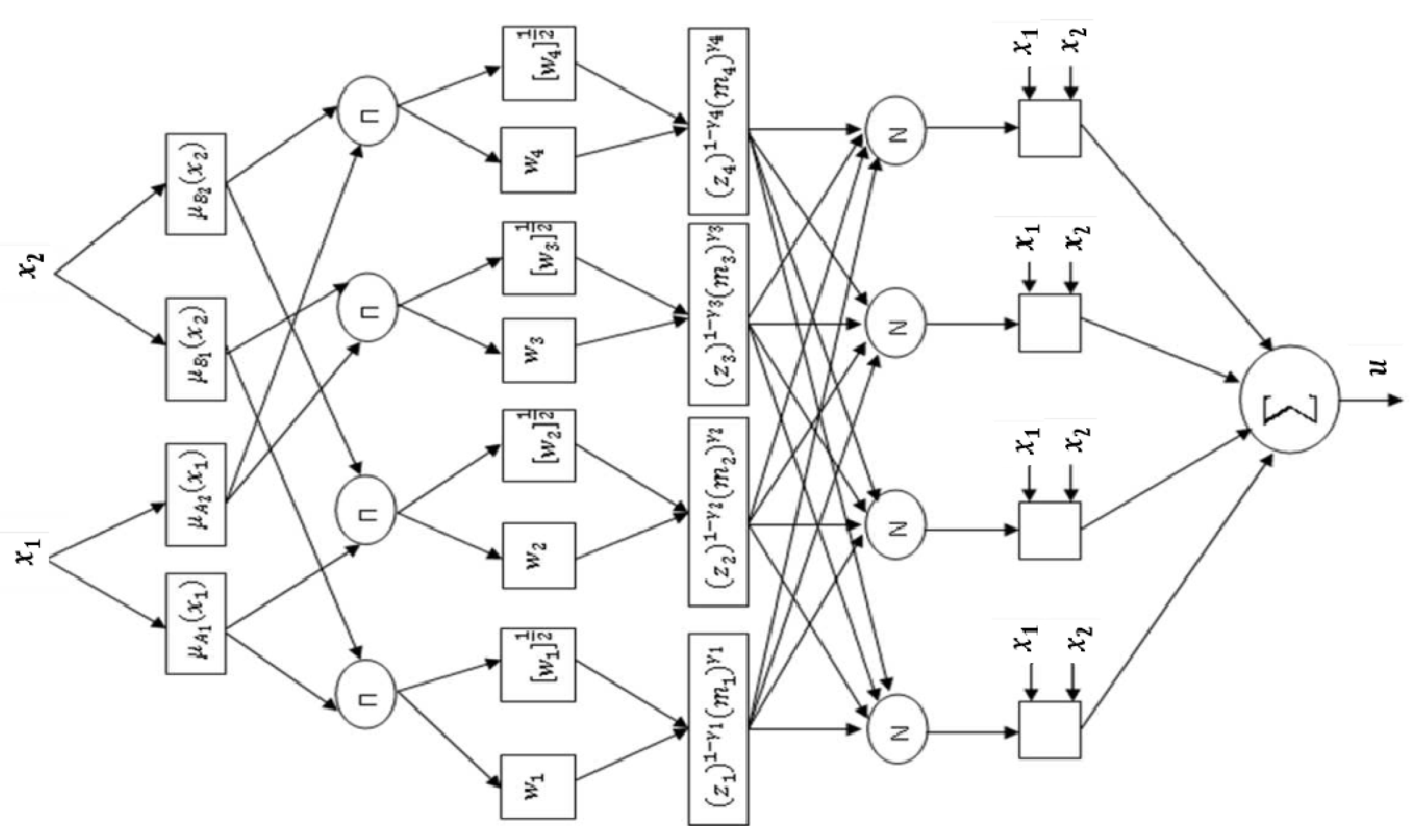
CANFIS is a fuzzy inference system based on a multi-layered adaptive network, where the learning algorithm not only adjusts the membership functions, but also optimizes the dynamics of fuzzy reasoning by adjusting the degree of compensation. In this section, we develop an ANFIS controller equipped with a fuzzy compensator, where the adaptation of its parameters is ensured by a learning algorithm based on the extended Kalman filter. To simplify understanding and without loss of generality, we consider a system with two inputs $x_1$, $x_2$ and one output $u$ (Figure 1), modeled by a fuzzy system of the Takagi–Sugeno type, composed of the following four fuzzy rules:

$$\mathrm{Rule}1:\mathrm{if}{x}_1\mathrm{is}{A}_1\mathrm{and}{x}_2\mathrm{is}{B}_1\mathrm{then}{u}_1=f_1\left(x_1,x_2\right)=a_1{x}_1+b_1{x}_2+c_1$$

(1)

$$\mathrm{Rule}2:\mathrm{if}{x}_1\mathrm{is}{A}_1\mathrm{and}{x}_2\mathrm{is}{B}_2\mathrm{then}{u}_2=f_2\left(x_1,x_2\right)=a_2{x}_1+b_2{x}_2+c_2$$

(2)

$$\mathrm{Rule}3:\mathrm{if}{x}_1\mathrm{is}{A}_2\mathrm{and}{x}_2\mathrm{is}{B}_1\mathrm{then}{u}_3=f_3\left(x_1,x_2\right)=a_3{x}_1+b_3{x}_2+c_3$$

(3)

$$\mathrm{Rule}4:\mathrm{if}{x}_1\mathrm{is}{A}_2\mathrm{and}{x}_2\mathrm{is}{B}_2\mathrm{then}{u}_4=f_4\left(x_1,x_2\right)=a_4{x}_1+b_4{x}_2+c_4$$

(4)

The degree of activation of a rule is defined by $w_i$.

We consider the pessimistic and optimistic operations, given respectively as follows:

$$z_i=w_i$$

(5)

$$m_i={\left(w_i\right)}^{\raisebox{1ex}{$1$}\!\left/ \!\raisebox{-1ex}{$2$}\right.}.$$

(6)

The fuzzy compensator expressed by this relation:

$$C_i(z_i,m_i,{\gamma }_i)={(z_i)}^{1-{\gamma }_i}{(m_i)}^{{\gamma }_i},$$

(7)

where ${\gamma }_i\in \left[0,1\right]$ is the compensatory degree. Therefore, the net value of the fuzzy neural-network equipped with a fuzzy compensator is given as follows:

$$u=\frac{{\displaystyle \sum _{i=1}^4\left(a_{i}e+b_i\Delta e+c_i\right)}{(w_i)}^{{\alpha }_i}}{{\displaystyle \sum _{i=1}^4{(w_i)}^{{\alpha }_i}}}$$

(8)

$${\alpha }_i=1-\frac{{\gamma }_i}{2}$$

(9)

Consider that $x_1$ and $x_2$ are the position error $e$ and its derivative $\Delta e$. We associate two fuzzy sets for each of the inputs, namely $N \left(Negative\right)$ and $P\left(Positive\right)$. ${\mu }_N$ et ${\mu }_P$ represent the appropriate membership degrees of the variables $x_i$ with respect to fuzzy subsets $A_i$ and $B_i$, defined by the following member functions:

$${\mu }_N(x_1)=\exp \left(-{\left(\frac{x_1-{\rho }_1}{{\sigma }_1}\right)}^2\right)$$

(10)

$${\mu }_P(x_1)=\exp \left(-{\left(\frac{x_1-{\rho }_2}{{\sigma }_2}\right)}^2\right)$$

(11)

$${\mu }_N(x_2)=\exp \left(-{\left(\frac{x_2-{\beta }_1}{{\delta }_1}\right)}^2\right)$$

(12)

$${\mu }_P(x_2)=\exp \left(-{\left(\frac{x_2-{\beta }_2}{{\delta }_2}\right)}^2\right),$$

(13)

with: $\left({\rho }_i,{\sigma }_i\right)$ and $\left({\beta }_i,{\delta }_i\right)$ being the (mean, variance) of the fuzzy set of the membership functions respectively of $x_1$ and $x_2$.

Learning Algorithm

The controller is characterized by a vector of parameters $\Phi$. Our objective is to find the values of the vector $\widehat{\Phi }$ by minimizing the following criterion [11]:

$$J(k)=\frac{1}{2}{\left(y_d(k)-y(k)\right)}^2=\frac{1}{2}{(e(k))}^2,$$

(14)

where: $y(k)$ is the real output of the system and $y_d(k)$ is its desired output. The extended Kalman filter approach consists of linearizing the output regulator $u_d$ at each step $k$ around the estimated vector ${\Phi }_d(k)$. This is equivalent to writing:

$$u_d(k)=u(k)+\mathsf{\Psi }(k)({\Phi }_d(k)-\Phi (k)).$$

(15)

With:

$$\mathsf{\Psi }(k)=\frac{\partial u(k)}{\partial \Phi (k)}=\left[\frac{\partial u(k)}{\partial {\Phi }_1(k)},\dots ,\frac{\partial u(k)}{\partial {\Phi }_n(k)}\right],$$

(16)

where $n$ is the dimension of the vector ${\mathsf{\Psi }}^T$. Consequently, the parameters are adjusted according to the following relation [12]:

$$\Phi (k+1)=\Phi (k)+K^{\prime }(k){\mathsf{\Psi }}^T(k)e_u$$

(17)

$$K^{\prime }(k)=\frac{P(k)}{\mathsf{\Psi }(k)P(k){\mathsf{\Psi }}^T(k)+B(k)}$$

(18)

$$P(k+1)=P(k)-K(k)\mathsf{\Psi }(k)P(k)$$

(19)

$$K(k)=K^{\prime }(k){\mathsf{\Psi }}^T(k),$$

(20)

where $\mathsf{\Psi }(k)$ is the Jacobian matrix (the observation matrix of the system), $P(k)$ is the estimation matrix of the error covariance and $B(k)$ is the measurement covariance matrix. In order to approximate the variation $e_u$, we linearize the inverse model of the system around $y(k)$ according to the following relation:

$$u=\frac{\partial u(k)}{\partial y(k)}\left(y-y(k)\right)+u(k),$$

(21)

where $y(k)$ is the system output and $u(k)$ its input. For this linearized model, the value $u_d(k)$ can be expressed as follows:

$$u_d(k)=\frac{\partial u(k)}{\partial y(k)}(y_d(k)-y(k))+u(k).$$

(22)

Therefore, we have:

$$u_d(k)-u(k)=\frac{\partial u(k)}{\partial y(k)}\left(y_d(k)-y(k)\right).$$

(23)

Then:

$$e_u(k)=\frac{\partial u(k)}{\partial y(k)}e(k).$$

(24)

We also have: $\partial e(k)=\partial y_d(k)-\partial y(k)$. We assume that $y_d(k)$ is constant in the neighborhood of $y(k)$. Then:

$$\partial e(k)=-\partial y(k).$$

(25)

Therefore:

$$e_u(k)=\frac{-\partial (k)}{\partial e(k)}e(k).$$

(26)

The relation (17) can be written as follows:

$$\Phi (k+1)=\Phi (k)K^{\prime }(k){\mathsf{\Psi }}^T(k)\frac{\partial u(k)}{\partial e(k)}e(k).$$

(27)

In order to eliminate the constraint ${\gamma }_i\in \left[\begin{array}{cc}0& 1\end{array}\right]$ defined in Equation (7), we define:

$${\gamma }_i=\frac{p_i{}^2}{p_i{}^2+q_i{}^2}.$$

(28)

Consequently, the parameters vector to be readjusted is given by:

$${\Phi }_i{}^T(k)=\left[a_1,b_1,c_1,p_1,q_1,\dots ,a_4,b_4,c_4,p_4,q_4\right]$$

(29)

$$\mathsf{\Psi }(k)=\left[\frac{\partial u(k)}{\partial a_1},\frac{\partial u(k)}{\partial b_1},\frac{\partial u(k)}{\partial c_1},\frac{\partial u(k)}{\partial p_1},\frac{\partial u(k)}{\partial q_1},\dots ,\frac{\partial u(k)}{\partial a_4},\frac{\partial u(k)}{\partial b_4},\frac{\partial u(k)}{\partial c_4},\frac{\partial u(k)}{\partial p_4},\frac{\partial u(k)}{\partial q_4}\right]$$

(30)

With:

$$\frac{\partial u}{\partial a_i}=\frac{e{\left[w_i\right]}^{{\alpha }_i}}{{\displaystyle \sum _{i=1}^4{\left[w_i\right]}^{{\alpha }_i}}}$$

(31)

$$\frac{\partial u}{\partial b_i}=\frac{\Delta e{\left[w_i\right]}^{{\alpha }_i}}{{\displaystyle \sum _{i=1}^4{\left[w_i\right]}^{{\alpha }_i}}}$$

(32)

$$\frac{\partial u}{\partial c_i}=\frac{{\left[w_i\right]}^{{\alpha }_i}}{{\displaystyle \sum _{i=1}^4{\left[w_i\right]}^{{\alpha }_i}}}$$

(33)

$$\frac{\partial u}{\partial {\gamma }_i}=-\frac{1}{2}\left[{\displaystyle \sum _{i=1}^4{a}_{i}e+b_i\Delta e+c_i}\right]\frac{z_i\ln (w_i)}{{\displaystyle \sum _{i=1}^4{z}_i}}$$

(34)

$$\frac{\partial u}{\partial p_i}=-\left[\frac{2p_i{(q_i)}^2}{{(p_i)}^2+{(q_i)}^2}\right]\frac{\partial u}{\partial {\gamma }_i}$$

(35)

$$\frac{\partial u}{\partial q_i}=\left[\frac{2q_i{(p_i)}^2}{{(p_i)}^2+{(q_i)}^2}\right]\frac{\partial u}{\partial {\gamma }_i}.$$

(36)

We have:

$$u=\frac{{\displaystyle \sum _{i=1}^4\left(a_{i}e+b_i\Delta e+c_i\right)}{(w_i)}^{{\alpha }_i}}{{\displaystyle \sum _{i=1}^4{(w_i)}^{{\alpha }_i}}}=\frac{h}{g}.$$

(37)

Then:

$$\frac{\partial u}{\partial e}=\frac{\frac{\partial h}{\partial e}.g-\frac{\partial g}{\partial e}.h}{g^2}.$$

(38)

With:

$$\frac{\partial h}{\partial e}={\displaystyle \sum _{i=1}^4\left(\left[a-2\left(e-{\rho }_j\right)\left(a_{i}e+b_i\Delta e+c_i\right)\right]w_i{}^{{\alpha }_i}\right)}$$

(39)

$$\frac{\partial g}{\partial e}=-2{\displaystyle \sum _{i=1}^4\left(\left(e-{\rho }_j\right)w_i{}^{{\alpha }_i}\right)},$$

(40)

where $j$ is the integer part of $(i-1)/2$.

3. Implementation of the CANFIS Controller Equipped with a Compensator on the Raspberry Pi 3 Board: Application on the Inverted Pendulum

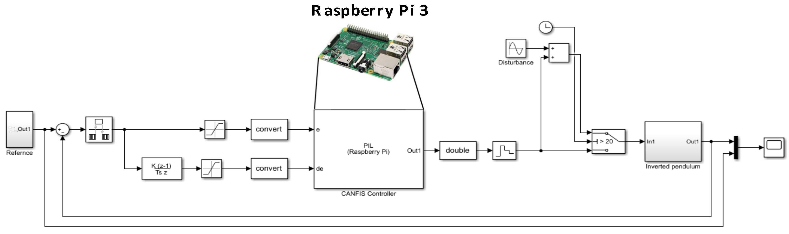
In this section, we use the “Processor-In-the-Loop” technique in MATLAB-Simulink, which allows us to test the behavior of the CANFIS controller on the Raspberry Pi 3 board [13]. In this mode of execution, the CANFIS controller runs in the hardware while the rest of the closed loop runs on the Simulink environment. In order to test the performances of the controller, we considered the stabilization problem of an inverted pendulum on a cart. The dynamic equations of the nonlinear system are given by [14]:

$${\dot{x}}_1=x_2$$

(41)

$${\dot{x}}_2=\frac{g\sin x_1-\cos x_1(\frac{ml}{m_c+m}{x}_2^2\sin x_1-\frac{1}{m_c+m}\tau (t))}{\frac{4}{3}l-\frac{ml}{m_c+m}{\cos }^2{x}_1},$$

(42)

where $x_1$ is the position of the vertical rod (in radian), $x_2$ is the angular velocity and $\tau (t)$ the torque applied to the rod. Its parameters are given in the

Table 1. Inverted pendulum parameters.

$g$	Gravity constant	9.8 m/s2
$m_c$	Carriage mass	1 kg
$m$	Pendulum mass	0.1 kg
$l$	Rod length	0.5 m

.

The implementation of the CANFIS controller was done with a frequency of 10 KHz. The execution diagram of the regulation chain (CANIFIS controller, System and disturbance) in PIL mode under the MATLAB Simulink environment is presented in Figure 2.

4. Results of the PIL Tests

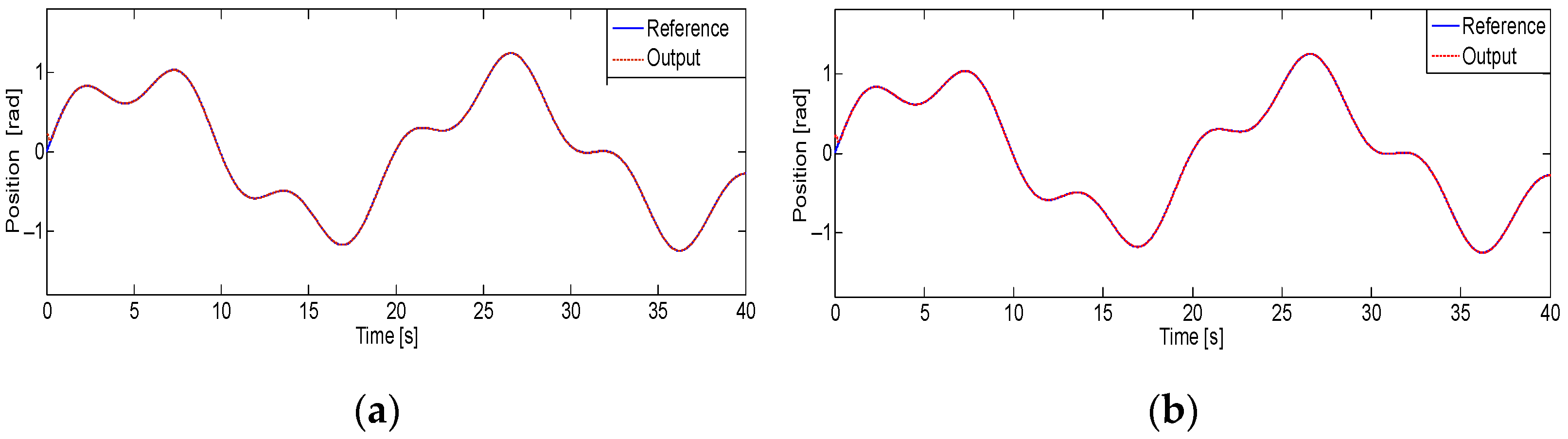
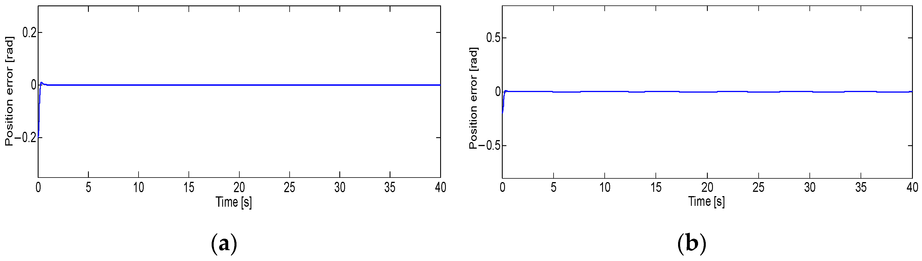
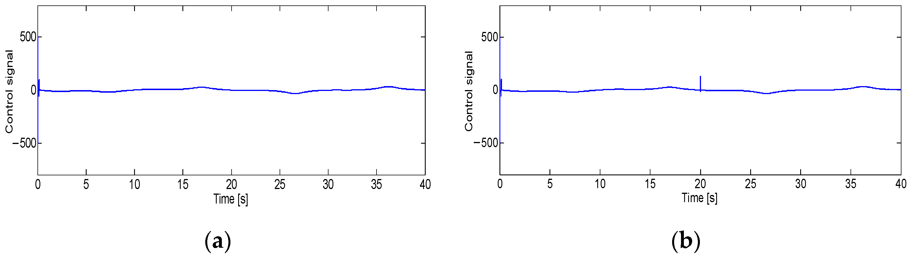
In this section, we present the simulation results of the PIL mode. In order to test the robustness of the two proposed controllers, we added a disturbance on the input of the system at the instant $t=20 \mathrm{s}$, given as follows:

$$D(t)=150\sin (t).$$

(43)

Figure 3a,b, Figure 4a,b and Figure 5a,b represent the results of the position tracking, the position tracking errors as well as the control signals delivered by the CANFIS controller. From these figures, we can see that the proposed controller has good performance (tracking, response time and robustness) with a low precision error, in both test cases (with and without disturbances). This is due to the use of a compensator which compensates for errors in the choice of membership functions, even readjusting the dynamics of fuzzy rules, using a learning algorithm based on the extended Kalman filter. The implementation of the proposed controller allowed us to obtain good performances thanks to the sampling frequency of the Raspberry Pi 3 board.

5. Conclusions

In this article, we have proposed the implementation on a Raspberry Pi 3 board of a neuro-fuzzy controller CANFIS, in order to control an inverted pendulum. The CANFIS controller presents good results because it uses a learning algorithm based on the extended Kalman filter, which converges very quickly, and which readjusts the membership functions and optimizes at the same time the dynamics of fuzzy reasoning by adjusting the degree of compensation. The development and implementation of the controller was done through MATLAB’s Simulink environment, which simplified the study and implementation of the code on the Raspberry Pi 3 board.

In conclusion, we have tried through this article to show the efficiency of the CANFIS controller on real hardware (Raspberry Pi 3) in the control of non-linear systems. The implementation of such a controller using the PIL technique has demonstrated its speed and robustness to disturbance rejection.

References

- Gil, P.; Oliveira, T.; Palma, L. Adaptive neuro–fuzzy control for discrete-time nonaffine nonlinear system. IEEE Trans. Fuzzy Syst. 2019, 27, 1602–1615. [Google Scholar] [CrossRef]
- Sarhadi, P.; Rezaie, B.; Rahmani, Z. Adaptive predictive control based on adaptive neuro fuzzy inference system for a class of nonlinear industrial processes. J. Taiwan Inst. Chem. Eng. 2016, 61, 132–137. [Google Scholar] [CrossRef]
- Song, S.; Zhang, B.; Song, X.; Zhang, Z. Adaptive neuro fuzzy backstepping dynamic surface control for uncertain fractional-order nonlinear systems. Neurocomputing 2019, 360, 172–184. [Google Scholar] [CrossRef]
- Song, S.; Park, J.H.; Zhang, B.; Song, X.; Zhang, Z. Adaptive command filtered neuro-fuzzy control design for fractional-order nonlinear systems with unknown control directions and input quantization. IEEE Trans. Syst. Man Cybern. Syst. 2020, 51, 7238–7249. [Google Scholar] [CrossRef]
- Mellah, R.; Khati, H.; Talem, H.; Guermah, S. Compensatory of adaptive neural fuzzy inference system. In Fuzzy Systems; IntechOpen: London, UK, 2021. [Google Scholar]
- Finnerty, A.; Ratigner, H. Reduce Power and Cost by Converting from Floating Point to Fixed Point; Xilinx All Programmable, v. 1.0; Xilinx, Inc.: San Jose, CA, USA, 2017; pp. 1–14. [Google Scholar]
- Karakuzu, C.; Karakaya, F.; Çavuşlu, M.A. FPGA implementation of neuro-fuzzy system with improved PSO learning. Neural Netw. 2016, 79, 128–140. [Google Scholar] [CrossRef] [PubMed]
- Khati, H.; Mellah, R.; Talem, H. Neuro-fuzzy control of a position-position Teleoperation system using FPGA. In Proceedings of the 24th International Conference on Methods and Models in Automation and Robotics, Miedzyzdroje, Poland, 26–29 August 2019; pp. 64–69. [Google Scholar]
- Khati, H.; Talem, H.; Mellah, R.; Bilek, A. Neuro-fuzzy control of bilateral teleoperation system using FPGA. Iran. J. Fuzzy Syst. 2019, 16, 17–32. [Google Scholar]
- Dorzhigulov, A.; Bissengaliuly, B.; Spencer, B.F.; Kim, J. ANFIS based quadrotor drone altitude control implementation on Raspberry Pi platform. Civ. Environ. Eng. 2018, 95, 335–345. [Google Scholar] [CrossRef]
- Mellah, R.; Guermah, S.; Toumi, R. Adaptive control of bilateral teleoperation system with compensatory neural-fuzzy controllers. Int. J. Control Autom. Syst. 2017, 15, 1–11. [Google Scholar] [CrossRef]
- Hayki, S. Kalman Filtering and Neural Networks; John Wiley and Sons Inc.: Hoboken, NJ, USA, 2001. [Google Scholar]
- Simulink Support Package for Raspberry Pi Hardware. User’s Guide; MathWorks, MATLAB and SIMULINK, r2021a; The MathWorks Inc.: Natikc, MA, USA, 2021. [Google Scholar]
- Yoo, B.; Ham, W. Adaptive fuzzy sliding mode control of nonlinear system. IEEE Trans. Fuzzy Syst. 1998, 6, 315–321. [Google Scholar]