1. Introduction
Providing an efficient simulation of air traffic flows is highly desirable, as there are many applications in air traffic management. Being able to randomly generate trajectories may serve to challenge the maximum capacity of airspaces, drive Monte Carlo simulations for collision risk estimation, or estimate levels of uncertainties within a route.
In general, trajectory generation methods can be divided into two main groups: model-driven and data-driven methods [
1]. Model-driven methods are based on flight dynamic equations, which have the advantage of guaranteeing the physical properties of a trajectory with respect to flight performances. Aircraft performance models such as BADA [
2] or OpenAP [
3] are particularly relevant for this aspect. However, such (mostly) deterministic methods struggle to take into account uncertainties introduced by various sources such as air traffic controllers (ATC) manoeuvres, human factors or meteorological conditions. Although sophisticated solutions exist [
4,
5,
6], model-driven methods always rely on assumptions that simplify reality.
Alternatively, data-driven methods leverage the statistical properties of observed paths and excel at imitating them. The Generative Adversarial Network (GAN) from Jarry et al. [
7] is a case in point. However, these methods require a large amount of data, are difficult to train, and may sometimes lack realism. Moreover, an inherent issue with these models is the evaluation of the
flyability of the generated trajectories, as there is no guarantee they follow the laws of physics. While en-route flights mostly consist of straight segments, terminal operation flows yield more complex shapes. Sudden changes in heading and altitudes are frequent, and ATC often take actions to deviate aircraft from the published procedures to respect separation rules and to optimize throughput. The resulting flows may contain high levels of variation, making data-driven methods more suitable than performance-based ones for the generation problem.
This paper focuses on the realistic reproduction of trajectory patterns for terminal manoeuvres, focusing on multivariate statistical distributions. Previous research already proposed various models to capture the distribution of flight deviations around a reference. Poppe and Buxbaum [
8] target the analysis of climb profiles by identifying nominal routes with clustering. Murça and de Oliveira [
9] modeled the distribution of flows approaching São Paulo airport with Gaussian mixtures models.
Dimensionality reduction is also an important challenge: Eckstein [
10] considered Principal Component Analysis (PCA) to project altitude and ground speed profiles into a lower dimensional space. Jarry et al. [
11] extended the process to continuous objects with functional-PCA. This study aims at combining these ideas and their extensions to the generation of 2D-paths for go-around trajectories at Zurich airport. Go-arounds on runway 14 are of particular interest, since the published procedure interacts with the standard instrument departure (SID) procedures for runway 16. The proposed method will rely on two steps:
Dimensionality reduction. This step focuses on finding a suitable representation space in which the analysis of the trajectories is simplified. In this paper, the emphasis was placed on the explainability and the intuition by taking a subset of the most relevant points of our initial route.
Distribution fitting. One of the most obvious ways to model flight flow is to estimate its statistical distribution. A multivariate joint distribution is fitted on the features previously constructed.
In the following,
Section 2 develops a way to better represent observed trajectories by selecting the most relevant positions.
Section 3 presents the different considered multivariate distribution estimation models. Metrics to evaluate the goodness of fit of the estimated distribution and the resemblance of the generated shapes with the reality are explained in
Section 4.
Section 5 details experiments which were conducted on Automatic Dependent Surveillance–Broadcast (ADS-B) data from the OpenSky Network [
12]. Perspectives for future work are discussed in
Section 6.
2. Global Approach
When it comes to modelling flight trajectories, stochastic processes appear to be the most appropriate tool: within a given flow, every flight is a realisation of the same random function. Blom et al. [
13] introduced randomness to flight mechanic equations to model trajectories in this way. This assumption is justified because terminal operation manoeuvres are most of the time driven by a standard procedure. Nevertheless, stochastic processes are complex and their estimation is often based on strong a priori knowledge. Observed trajectories are finite and discrete, and simplifications can be made using multivariate distributions. Flights are not considered as realisations of a random function anymore, but as realisations of a random vector. Methods to estimate multivariate distributions are many, but given the specificity of trajectories, statistical copulas seem attractive: they allow for the separation of the estimation of each marginal distribution and its dependencies. However, the higher the dimension, the weaker the goodness of the fit. This section focuses on finding an adapted discrete representation that reduces the dimension of the estimated multivariate distribution, without losing information.
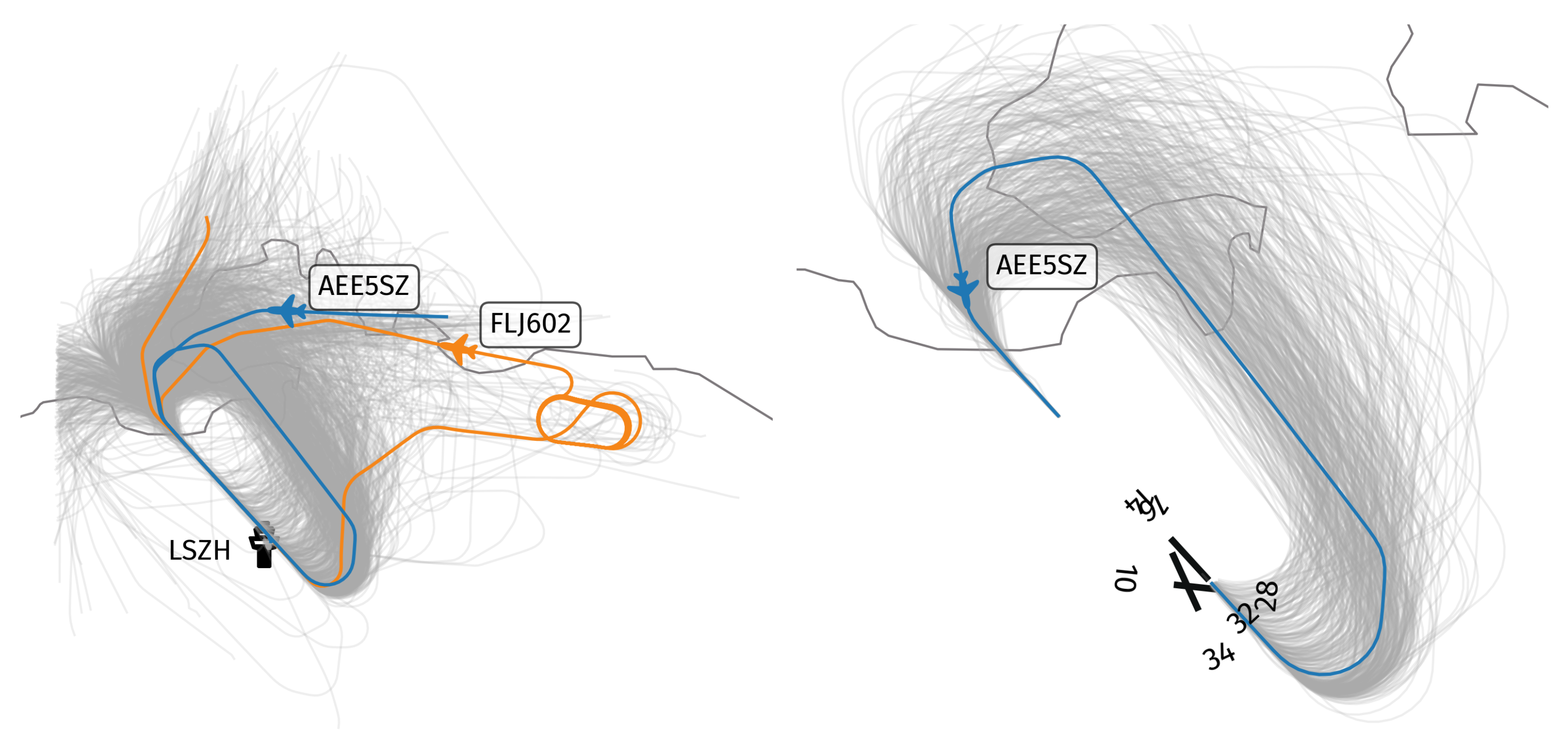
2.1. Removal of Outliers
Three years of observations of 646 go-around situations at the Zurich Airport between January 2017 and December 2019 were collected. Among those, we selected only runway 14 go-arounds and removed the few trajectories which did not follow the standard missed approach procedure. That includes the paths on the turns in the wrong direction, the early procedures and the holding patterns. Eventually, we normalized the beginning and the ending of each trajectory to the end of runway 14, and 1.5 nautical miles after the final approach fix, respectively.
The resulting flow, displayed in
Figure 1, is comprised of 407 trajectories. Consequently, we have a consistent representation of trajectories, with the same beginning and ending points, and avoid dealing with patterns that are too atypical, which are to be considered in future works.
2.2. Feature Selection
Even though a formal trajectory is a continuous curve, an observed trajectory is discrete and can be defined as where n is the number of observations and their spatial positions. As a result, a trajectory is represented by a vector of random variables . Nevertheless, each trajectory has a different length and sampling naively (cutting each trajectory into n equal parts) can be problematic: the i-th observation of one trajectory does not necessarily match the same flight phase as the i-th observation of another. Moreover, when it comes to fitting multivariate distributions, reducing the number of dimensions to the minimum is often considered good practice. The method developed in this section consistently represents a trajectory with n variables instead of , without any loss of information, in a way that every i-th coordinate correspond to the same flight phase.
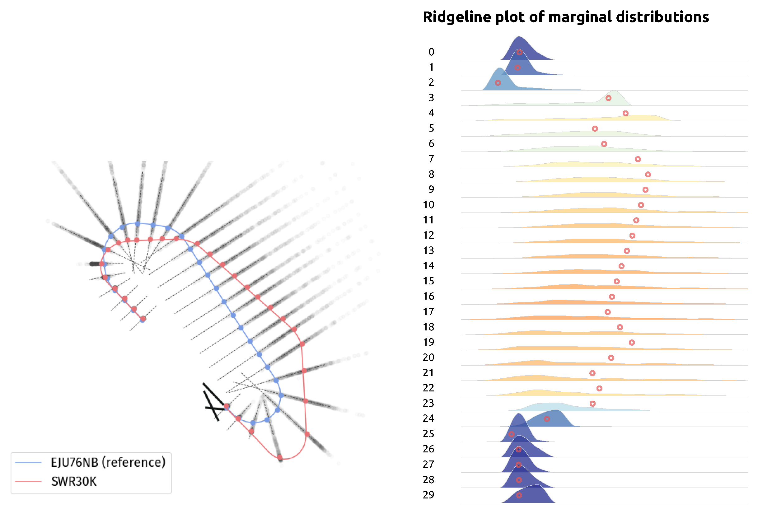
First, we select a suitable reference trajectory that is resampled naively into the desired number of n features: its choice is important as it should have a very regular shape, such as a standard go-around trajectory. Then, we calculate the normal line to the selected curve in every point and resample the other trajectories by taking their intersections with these lines. Due to atypical shapes during the initial and final turns, the intersection may in some cases not exist, or the candidate point may be too far from the previously selected one. Shall it arise, we just pick the first position after the previously selected one.
As a result, every trajectory is exactly represented by only
n points, and the positions
of all the trajectories are on the same line, as shown in
Figure 2 (left). The main benefit is that the coordinate
of a point can be directly deduced by its
. Features are no longer
but
where
is the projection of
on the
i-th normal line. Due to the approximations in the algorithm, some points may not be exactly aligned but are so close one can assume they are. Thus, the marginals are the statistical distributions of the points along each line displayed in
Figure 2 (right) and the dependencies between them can be captured by a statistical copula. All together, they form the joint distribution of the random vector
representing a trajectory. This projection method allows us to reduce the number of features by a factor of two without any loss of information and provides a very intuitive and visual way to (partially) address the large dimension.
3. Multivariate Density Estimation
Section 2 discussed a way to reduce the dimension of the problem by representing trajectories with realisations of a random vector of size
n. Generally speaking, estimating the underlying multivariate distribution is no easy task, and existing methods often struggle to quantify the dependencies as the dimension increases. This section details the most common models to learn
d-variate distribution of the random vector
from
N independent and identically distributed realisations. Depending on the application of the dimension reduction method or not,
or
. In the following, notations using bold mathematical quantities are vector quantities, while the others are scalar.
3.1. Multivariate Gaussian and Gaussian Mixtures
While many distribution families are available for the parametric estimation of unidimensional laws, few can be directly extended to the multivariate case. Thus, the multivariate normal distribution (MVN) is often the ground method and is parameterized by a mean vector
and its covariance matrix
. They are estimated using maximum likelihood method applied on the available
N-sample. It assumes that every linear combination of the Gaussian vector is Gaussian, and more specifically, that every components is Gaussian. According to
Figure 2, that is not the case for the samples of
Section 2. Moreover, the increase in dimension may induce too complex dependencies between the marginals to be modeled by the correlation matrix. To improve the estimation and to capture more refined dependency patterns, a Gaussian mixture model (GMM) can be considered. The density is defined by:
where
and
is a multivariate normal density with mean
and covariance matrix
. These parameters are estimated from the
N observed trajectories with the expectation-maximization (EM) algorithm [
14] to find the maximum likelihood, and the number of components
k is chosen so as to have the most accurate estimate, while avoiding over-fitting using the Bayesian information criterion (BIC) minimization.
3.2. Statistical Copulas
Statistical copulas allow to disentangle the estimation process into a number of simpler tasks; estimating the individual behaviour of the features with the marginal distributions, and the dependence between the marginals with the copula function.
Theorem 1 (Sklar).
Sklar’s Theorem [15] states that every multivariate cumulative distribution function F of a random vector can be expressed in terms of its d marginals and a function called copula:when the marginals are continuous, C is unique. The converse of the theorem is also true. Marginal distributions are easy to estimate as they are 1-dimensional densities, and a plethora of methods can be used: maximum likelihood, kernel density estimation or empirical distribution are cases in points. As enough data are available, empirical distribution is used to avoid errors of modelling.
The estimation of the statistical copula C is often more complex when the dimension d increases. Most of the time, for a given family of copulas , one may estimate the best parameter with parametric methods, e.g. maximum likelihood. Nevertheless, even though there are many families of bivariate copulas, only few of them are available for higher dimensions. As a result, even if we have powerful tools for bivariate estimation, they lose accuracy and flexibility when employed for higher dimensional ones.
As a consequence, models have been developed to take advantage of the knowledge of two-dimensional copulas. The most known technique is the
vine copula which was described for the first time by Joe [
16]. They decompose high-dimensional copulas into a product of conditional bivariate ones using the Bayes Theorem, each being fitted independently. Decomposing the high-dimensional model into a composition of smaller ones allows one to increase the degrees of freedom, and thus to grasp more complex dependencies. The decomposition patterns are not unique, and can be represented by a set of trees, where the
i-th tree is directly deduced by the
-th. Therefore, the whole model is determined by the first tree, and choosing the right one is an important task. Even though algorithm can automatically select it, leveraging the prior knowledge of the data saves time and accuracy. In the case of an aircraft trajectory, the
i-th position depends on the
-th, and the corresponding vine copula model is called D-vine.
4. Metrics
To evaluate the generative process, several aspects have to be taken into account such as the shape of the generated trajectory and the goodness of fit. The former aims to translate mathematically the perception of a human being about realistic generations by focusing on the roughness. The latter deals with the ability of the generation method to reproduce the statistical distribution of the initial dataset.
4.1. Curvature Variation
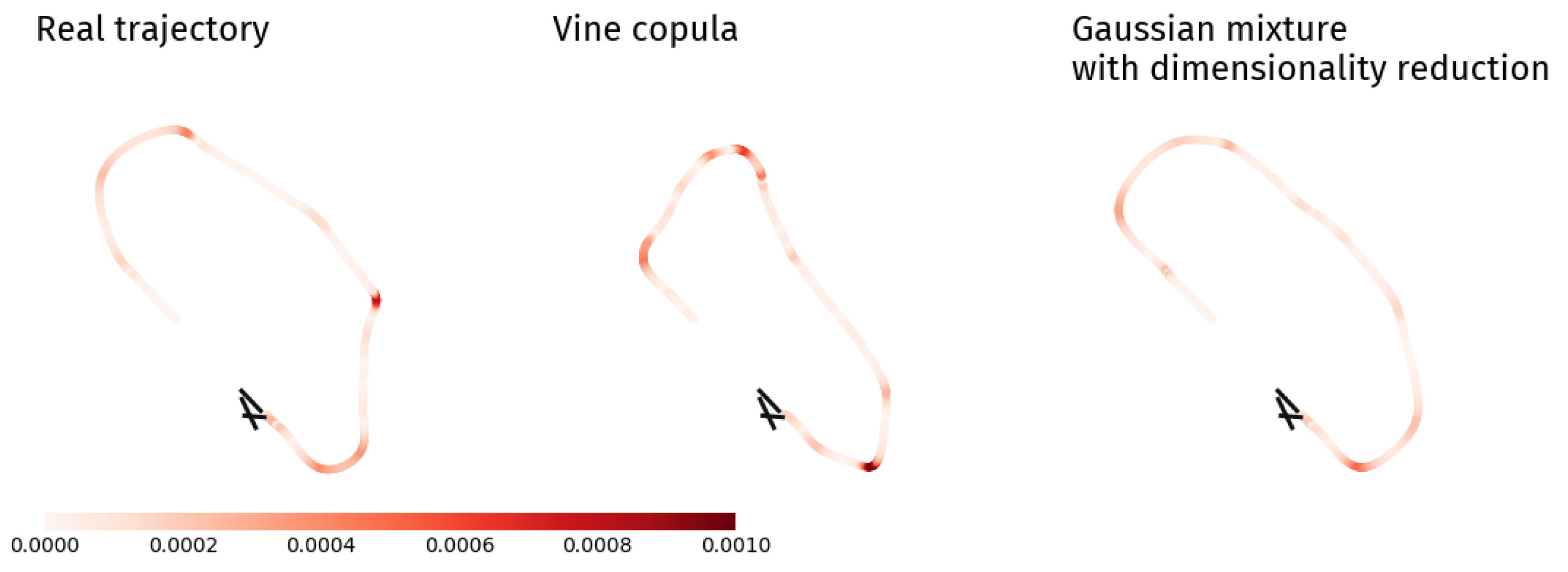
Moreton [
17] provides an extensive set of tools to analyse curves. It appears that an aircraft trajectory is mostly composed of straight lines connected by turns, and embodies well the characteristic of minimum curvature variation. The desired aircraft path should not be wiggly, and to quantify that, the proposed measure counts the number of times the curvature exceeds a threshold. Some examples are displayed in
Figure 3.
4.2. Goodness of Fit
The most straightforward way to ensure the generated trajectories are realistic is to quantify how well the estimated statistical model fits a set of observed trajectories. In other terms, those metrics evaluate the ability of the model to render the statistical characteristics of the original dataset.
The two first metrics used are based on the Mahalanobis distance. Unlike the Euclidean distance where every component is taken independently, the Mahalanobis distance gives less weight to the more dispersed ones. For our work, we will consider the two following variants
and
. Let denote the
-samples
of generated trajectories
and the
-samples
of real trajectories of the dataset
. The mean and the covariance matrix of the samples
is assumed to be equal respectively to
and
. The mean distance
of the generated trajectories to the mean of the real dataset is defined as
The second quantity we will estimate is the mean distance
of a generated trajectory to every real trajectory, i.e
The distance
quantifies the ability of the generation method to produce trajectories in the denser part of the distribution, whereas the term
renders the ability to generate trajectories close to the existing ones.
Székely et al. [
18] propose another metric based on expected values of the Euclidean distances between random vectors. The aim is to determine if two sets of different length of random vectors follow the same distribution. Let define
the Euclidean norm on
. The
e-distance between
and
is given by:
If the sets are identically distributed, the distance tends asymptotically to a positive constant, whereas it tends to the infinity if they are not. As a result, a large e-distance corresponds to different distributions, and provides a measure of the distance between them. It will be used to measure the gap between the database, and the generated set of trajectories.
5. Experiment and Results
Let us note that depending on the application of the dimensionality reduction (DR), the generated datasets have resp. or features. Nevertheless, comparing distances made on objects of different dimensions is not relevant, and thus when the dimension reduction has been used, the inverse transformation has been applied before calculating the metrics. Therefore, they quantify the goodness of fit and the ability of the DR method to maintain the statistical properties.
Table 1 summarizes the performance metrics for the different models. It contains the mean number of turns, the Mahalanobis distance to the mean of the observed data
, the mean Mahalanobis distance to every trajectory from the real data
, and the e-distance. For each method, 100 sets of 1000 trajectories have been generated, and the mean for each metric have been calculated.
Figure 4 shows the corresponding barplot.
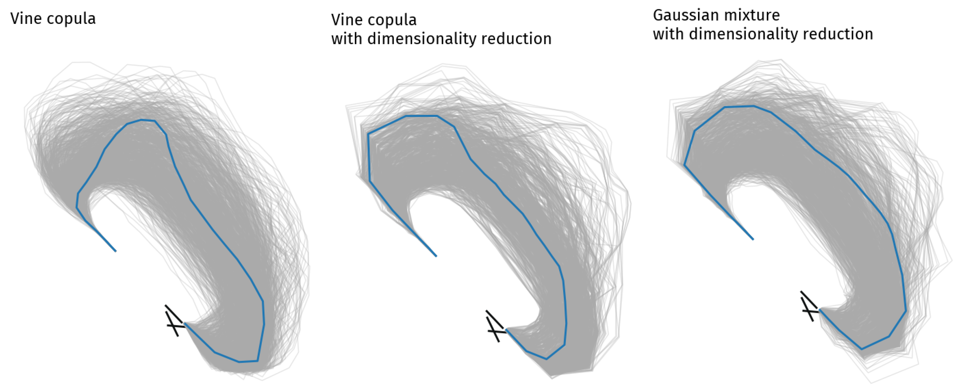
The DR method increases significantly the goodness of fit. It reduces the e-distance and
. The generated set is then statistically closer to the real flow, and the generated trajectories are on average less atypical. Those results can be also seen on
Figure 5: the flow generated without DR (on the left) have trajectories that run too close to the airport with an initial turn that is often too sharp. It also fails to recreate the region far away from the airport. The two other flows (on the right) have more realistic shapes.
The mean number of turns calculated for the real trajectories dataset is 7.9, and both GMM and MVN without DR give very close results. Covariance matrices from Gaussian distributions are less complex than the dependency pattern of a vine copula, and may actually filter the wiggles. However, the DR increases the number of turns and
. This reflects the fact that this processing induces wiggles within the generated trajectories. The method described in
Section 2 actually contains few approximations to deal with some uncommon cases, and selected points may sometimes not be on the exact same line, whereas the reverse transformation supposes it. Then, the dependency learned within the latent space may slightly be distorted by the reverse transformation.
Because of its strong assumptions, the MVN gives the worst results in every way. GMM and vine copulas appears to be close, but the former estimates better the overall distribution, and provides less wiggly trajectories. GMM generates more realistic shapes on average. The copula is certainly the most sensitive method to the large dimension, and it also observes the greater improvement when using the DR. Their main drawback comes from the estimation of the area around the center of the flow; i.e. the standard procedure area. As seen on
Figure 5, GMM provides a denser area for the same number of generated trajectories.
6. Conclusions and Future Works
This research work aims at modelling aircraft flows with multivariate distributions. A dimension reduction method has been developed to reduce the number of features by a factor of two without any loss of information. All positions are distributed along the normal line to a reference trajectory and represent the marginal distributions. Copulas, estimated here by a D-vine model, appeared to be a suitable tool as they directly map the set of the marginal distributions into the joint distribution. They were compared to multivariate normal distribution and Gaussian mixtures models.
Reducing the number of dimensions is a core issue, and the method from
Section 2 significantly improved the goodness of fit (see e-distance and Mahalanobis to mean metrics), but also introduced wiggles into the generated trajectories materialized by the number of turns and the mean Mahalanobis metrics. Moreover, limits of the approach were met with trajectories with loops or significantly atypical behaviours. Future work will focus on trajectory representations in lower dimension space, where information loss is acceptable, and in which fitting a multivariate distribution is more straightforward. In addition to generalising to more complex trajectories, this would also improve the estimation of the distribution.
As this paper focused on the reproduction of two-dimensional lateral shapes of an aircraft trajectory, future works will also generalise the approach to four-dimensional trajectories:
where
n is the number of observations,
their spatial positions and
time, leading to a larger number of features
. This increase in dimensions raises new issues about the dimension reduction method in
Section 2, about multivariate distribution models that are more likely to fail, and about the impact of aircraft types on 4-D trajectories. Hybrid methods merging data and model-driven generation could be a way to address these limitations.
In this preliminary work, D-vine copulas were slightly outperformed by Gaussian mixtures. Even though they are well suited to the approach, they seem to suffer from high dimensions more than the other models. Vine models are by far the most used technique to estimate a copula. However, their use is limited to a dozen variables in practice, and the 30 features considered here are certainly too much. Other copulas fitting models could be considered, and to that extent, leveraging the flexibility of Deep Learning methods could allow us to look into a more diversified function space to build more complex copulas.
Author Contributions
Conceptualization, all; methodology, T.K., J.M. and X.O.; software, T.K.; validation, T.K.; formal analysis, T.K., J.M. and X.O.; investigation, T.K.; resources, all; data curation, T.K.; writing—original draft preparation, T.K.; writing—review and editing, all; visualization, X.O.; supervision, J.M and X.O.; project administration, B.F. and R.M.; funding acquisition, B.F. and R.M. All authors have read and agreed to the published version of the manuscript.
Funding
This work was supported by the Swiss Federal Office of Civil Aviation, grant number BAZL SFLV 2018-037.
Data Availability Statement
References
- Olive, X.; Sun, J.; Murca, M.C.R.; Krauth, T. A Framework to Evaluate Aircraft Trajectory Generation Methods. In Proceedings of the 14th USA/Europe Air Traffic Management Research and Development Seminar, New Orleans, LA, USA, 20–24 September 2021; p. 10. [Google Scholar]
- Nuic, A.; Poles, D.; Mouillet, V. BADA: An advanced aircraft performance model for present and future ATM systems. Int. J. Adapt. Control. Signal Process. 2010, 24, 850–866. [Google Scholar] [CrossRef]
- Sun, J.; Hoekstra, J.M.; Ellerbroek, J. OpenAP: An Open-Source Aircraft Performance Model for Air Transportation Studies and Simulations. Aerospace 2020, 7, 104. [Google Scholar] [CrossRef]
- Soler, M.; Olivares, A.; Staffetti, E. Hybrid optimal control approach to commercial aircraft trajectory planning. J. Guid. Control. Dyn. 2010, 33, 985–991. [Google Scholar] [CrossRef]
- Patel, R.B.; Goulart, P.J. Trajectory generation for aircraft avoidance maneuvers using online optimization. J. Guid. Control. Dyn. 2011, 34, 218–230. [Google Scholar] [CrossRef]
- Kamgarpour, M.; Dadok, V.; Tomlin, C. Trajectory generation for aircraft subject to dynamic weather uncertainty. In Proceedings of the 49th IEEE Conference on Decision and Control (CDC), Atlanta, GA, USA, 15–17 December 2010; pp. 2063–2068. [Google Scholar]
- Jarry, G.; Couellan, N.; Delahaye, D. On the use of generative adversarial networks for aircraft trajectory generation and atypical approach detection. In Proceedings of the 6th ENRI International Workshop on ATM/CNS, Tokyo, Japan, 29–31 October 2019. [Google Scholar]
- Poppe, M.; Buxbaum, J. Clustering Climb Profiles for Vertical Trajectory Analysis. In Proceedings of the 10th SESAR Innovation Days, Virtual, 7–10 December 2020. [Google Scholar]
- Murça, M.C.R.; de Oliveira, M. A Data-Driven Probabilistic Trajectory Model for Predicting and Simulating Terminal Airspace Operations. In Proceedings of the 39th IEEE/AIAA Digital Avionics Systems Conference (DASC), San Antonio, TX, USA, 11–15 October 2020. [Google Scholar]
- Eckstein, A. Data driven modeling for the simulation of converging runway operations. In Proceedings of the 4th International Conference on Research in Air Transportation, Budapest, Hungary, 1–4 June 2010. [Google Scholar]
- Jarry, G.; Hassoumi, A.; Delahaye, D.; Hurter, C. Interactive Trajectory Modification and Generation with FPCA. In Proceedings of the ICRAT 2020 9th International Conference for Research in Air Transportation, Tampa, FL, USA, 23–26 June 2020. [Google Scholar]
- Schäfer, M.; Strohmeier, M.; Lenders, V.; Martinovic, I.; Wilhelm, M. Bringing up OpenSky: A large-scale ADS-B sensor network for research. In Proceedings of the IEEE IPSN-14 13th International Symposium on Information Processing in Sensor Networks, Berlin, Germany, 15–17 April 2014; pp. 83–94. [Google Scholar]
- Blom, H.; Bakker, B.; Everdij, M.; Van Der Park, M. Collision risk modeling of air traffic. In Proceedings of the IEEE 2003 European Control Conference (ECC), Cambridge, UK, 1–4 September 2003; pp. 2236–2241. [Google Scholar]
- Reynolds, D.A. Gaussian mixture models. Encycl. Biom. 2009, 741, 659–663. [Google Scholar]
- Sklar, M. Fonctions de répartition à n dimensions et leurs marges. Publ. Inst. Statist. Univ. Paris 1959, 8, 229–231. [Google Scholar]
- Joe, H. Families of m-variate distributions with given margins and m (m − 1)/2 bivariate dependence parameters. Lect. Notes-Monogr. Ser. 1996, 28, 120–141. [Google Scholar]
- Moreton, H.P. Minimum Curvature Variation Curves, Networks, and Surfaces for Fair Free-Form Shape Design. Ph.D. Thesis, University of California, Berkeley, CA, USA, 1992. [Google Scholar]
- Székely, G.J.; Rizzo, M.L. Testing for equal distributions in high dimension. InterStat 2004, 5, 1249–1272. [Google Scholar]
| Publisher’s Note: MDPI stays neutral with regard to jurisdictional claims in published maps and institutional affiliations. |
© 2021 by the authors. Licensee MDPI, Basel, Switzerland. This article is an open access article distributed under the terms and conditions of the Creative Commons Attribution (CC BY) license (https://creativecommons.org/licenses/by/4.0/).


