1. Introduction
Predictability is the cornerstone of air traffic management (ATM). Ensuring predictable operations allows for the optimization of security, operational efficiency and environmental sustainability by defining optimal schedules, interactions and resource allocation. However, most of these operations depend on many factors that might not be confidently predicted, such as weather conditions or unexpected delays in departures or arrivals. The volume and complexity of these operations are also a challenge. In many cases, the amount of information and effort that is needed to accomplish this goal can exceed human capacities [
1]. In these cases, automatic learning systems based on historical data may provide valuable support to air traffic management.
Management of incoming and outgoing flights in the surroundings of an airport is one of the more complex and risky tasks that need to be tackled. Knowing beforehand when an aircraft is going to approach the airport is key to plan the exact timings and resource allocation for the flights that need to be managed in the short-term future. This task is known as estimation of the time of arrival: at any moment of the flight, it is necessary to estimate accurately when the aircraft is going to arrive at the destination airport (that is, predict the estimated time of arrival or ETA), or the amount of time remaining before the flight ends. To this end, knowing both the current state of the flight and how it has progressed since its departure might contribute to improve the accuracy of the ETA prediction. A natural way for representing this data can be given as 4D-trajectories.
In recent years, 4D-trajectories have become prominent to represent flight data, influenced by the guidelines established in SESAR and NEXTGEN initiatives. This representation describes a flight as a succession of 3D position points (latitude, longitude and altitude) with an associated timestamp [
2]. Therefore, it allows for the identification as to where and when an aircraft is located. 4D-trajectories may also be further enriched with data about the state of the flight along the trajectory. This data might be informative about the evolution of the flight, and how the circumstances of a flight can influence its performance.
Modeling flight data as 4D-trajectories allows us to approach ETA prediction as a time series problem. Given a segment of a trajectory, we need to predict how it is going to evolve in the future. A wide variety of techniques have been applied to this problem, and machine learning approaches have yielded promising results [
3,
4]. In this paper, we focus on predicting the estimated time of arrival at a particular airport (Madrid Barajas-Adolfo Suárez) using deep learning and surveillance data. In particular, we propose different models based on LSTM networks [
5]. These networks are characterized by their ability to capture temporal dependencies in long sequences of data. This can be used with surveillance data to make accurate ETA predictions at any instant of an ongoing flight.
The remainder of this paper is organized as follows. In
Section 2 we provide an overview of previous work on ETA estimation, as well as a succinct description of the techniques that have been used on this task.
Section 3 describes the datasets that will be used for model training and evaluation in this work. In
Section 4 we describe the models used to evaluate, and the metrics that will be used to do so. The results will be presented and discussed in
Section 5. Finally,
Section 6 describes our main conclusions and future work.
2. Background
In the last decades, machine learning has been applied in many proposals to calculate ETAs for commercial flights using historic trajectory data. Algorithms such as GBM (Gradient Boosting Machines) [
6] or ADABoost [
7] have proved to be effective to provide accurate predictions at different time horizons or distances [
8], or even before the flight takes off [
4]. Models are usually designed specifically for predicting flights in a route between pairs of airports, [
4], flights landing on a particular runway configuration [
9], or trajectories in the surroundings of a particular airport [
8,
10].
Many factors may influence the progress of a flight, thus making the actual time of arrival diverge from that scheduled in the flight plan. This motivates the variety of features that have been applied to improve ETA predictions. Surveillance data (mainly ADS-B data) is present in most of the proposals: GPS position, altitude, speed and heading are relevant features to describe the movement over time of the aircraft. Weather conditions (such as wind direction and speed, or visibility), whether at the airport of origin or destination [
8] or all along the route [
4], are also key factors that influence the arrival time. Flight plan data [
3,
11] may help in the design of the models or be used as input data, by informing of the origin and destination airports, the (scheduled and actual) off-block and take off times (if the flight has already started), the scheduled arrival time, or the expected total duration of the flight. Finally, some features aim to leverage the temporal regularity of the operations by including data about day of the week, the month or the time of the day in which the flight will occur [
3]. Different metrics about air traffic density (number of landing or take-off operations) and resource management (configuration of runways) may also be useful in this task [
10].
Deep learning approaches have also been used for ETA prediction [
4]. However, it is known that deep learning algorithms are data-greedy, and many relevant data sources are not free and open, or do not provide enough data to train functional deep learning models. Therefore, it is relevant to explore how open sources like OpenSky Network [
12] may be leveraged to train such models.
RNNs are commonly used to learn from sequences of temporal data. Unlike feed-forward networks, RNNs also define connections between units in the same layer, which enables them to exhibit some “memory” from previous temporal instants. However, this causes RNNs to form very deep structures that increase the risk of vanishing gradients [
13]. To overcome this problem, LSTM (short for Long-Short Term Memory) networks [
5] proposed a novel neuron structure that ensures a correct propagation of the error, thus enabling the network to capture long-term temporal relations.
LSTM networks often present a single layer of LSTM units, and a Dense layer to adequately format the expected output. This structure is commonly known as a
vanilla LSTM network. However, we can arrange multiple LSTM layers to form
stacked or
deep LSTM networks. These are more complex models with larger capacities which might help in the learning of temporal patterns in the input sequences at different levels [
14].
LSTM layers can also be combined in an Encoder-Decoder architecture [
15]. Encoder-decoder architecture has been applied before in ATM for anomaly detection in ADS-B signals. The model learns from historical temporal patterns from existing trajectories, and tries to discover anomalous sequences (e.g., man-in-the-middle attacks) based on their similarity with the predicted sequence [
16]. They have also been applied for multivariate time-series forecasting [
17]. Encoder-decoder models are comprised of two different networks: an encoder that processes input data and converts it into a fixed-lenght representation. and a decoder that receives the resulting hidden state of the encoder.
In this work, we propose a different approach from traditional applications of LSTM networks for multivariate regression problems. We aim to learn from multiple time series (i.e., aircraft trajectories), instead of predicting new values in a time series based on past values. There are two main challenges that might interfere with this goal. First, state vectors are not evenly distributed in time. It is common that time series data are delivered at a regular and fixed frequency. ADS-B data depends on having at least one receiver in the range to be captured and registered, and individual messages are timestamped by the receiver at the capture moment. Thus, there is a high degree of stochasticity in the registration time of the data due to variable distances, transmission conditions and even receiver capacity, and adding noise to the temporal dimension of the problem. Secondly, time series data coming from different trajectories might be very different, even if they belong to the same route and are made in similar conditions (meteorology, schedules, aircraft). This might exceed the capacity of simpler models, and therefore require more complex models than the ones presented here.
3. Data
This section describes the data that will be used to predict ETAs, and the transformation operations that are applied to adapt these data for their use in the models.
3.1. Dataset Description
Each airport presents particular conditions (localization, meteorology, physical runways and configurations, traffic volume, etcetera), and therefore it would require additional data and more complex models to adapt to this increased variability. Our study focuses on flights arriving at Madrid Barajas-Adolfo Suárez Airport (ICAO code: LEMD).
We constructed a dataset of surveillance data from flights that arrived at Madrid Barajas-Adolfo Suárez from the 8th through the 28th of January, 2020. We chose this period to (1) avoid the Christmas holidays that take place up to the 6th of January in Spain and could distort the data, and (2) work with a situation of normality prior to the effects that COVID-19 has had on air traffic during 2020 and 2021. Using three weeks of data will allow us to exemplify the complexity of flight data and leverage some of the existing temporal patterns (daily and weekly) present in this kind of data. Surveillance data typically include time and 3D position data (latitude, longitude and altitude), which are the basis for describing a 4D trajectory. Sources like ADS-B provide further flight state information, but their use is beyond the scope of this work. Additionally, we generate some auxiliary features to further describe the temporal and positional context of the flight, which are described in the next section.
3.2. Data Acquisition
We used the OpenSky Network [
12] as the main data source. We also used flight plan data from Network Manager (
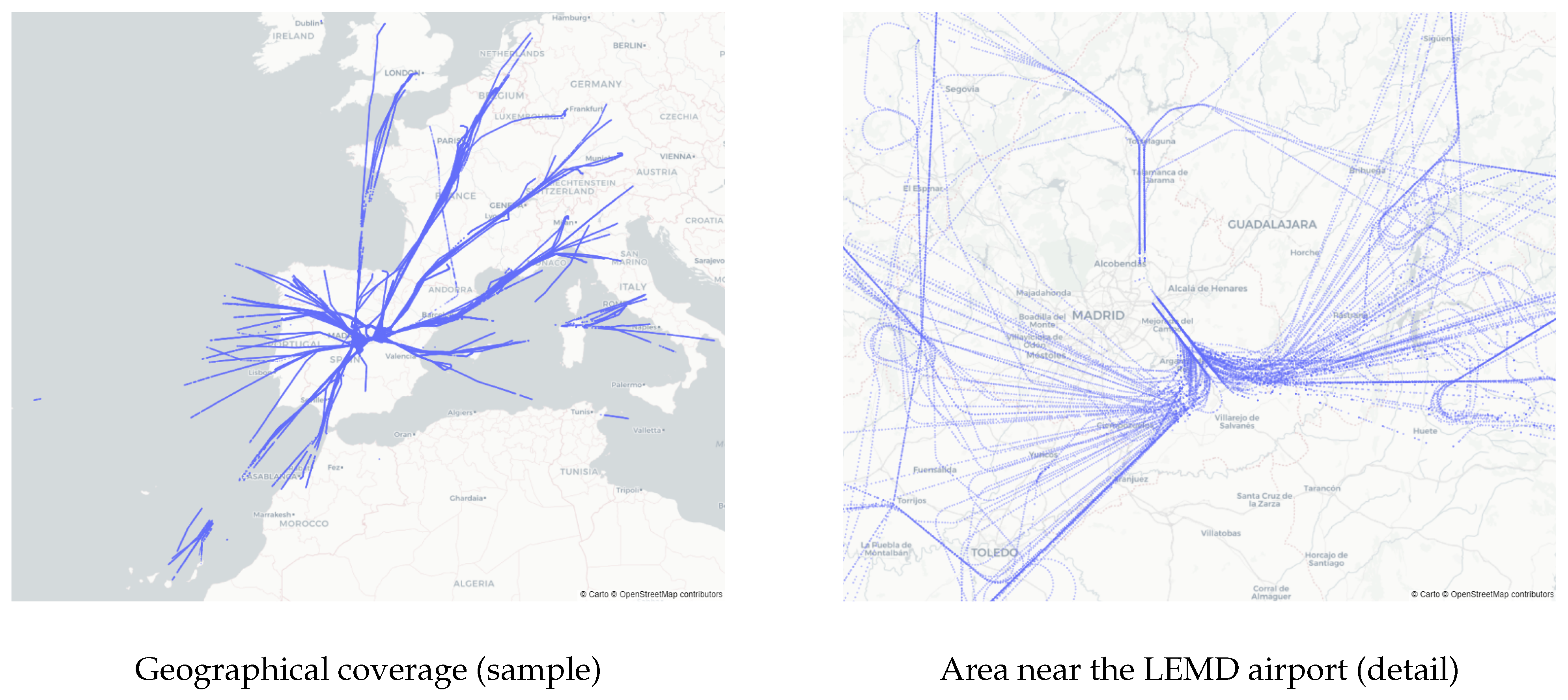
https://www.eurocontrol.int/network-operations, accessed on 17 November 2021) (managed by EUROCONTROL) to help to identify individual trajectories in the raw OpenSky data, and provide a landing time whenever it can not be inferred from ADS-B data. A total of 9190 flights are included in the dataset, of which 2118 correspond to domestic flights (flights coming from other Spanish airports) and 7072 to international flights.
Figure 1 displays an overview of the geographical coverage (left) and the vector density (right) of the dataset.
3.3. Data Preparation
We focus only on the last two hours of the flights to reduce the impact of heavily incomplete trajectories in the dataset, such as flights coming from South America across the Atlantic. Differences in length between domestic and international trajectories are reduced too. This is accomplished by removing state vectors with RTAs greater than 7200 s. We then apply a simple data cleaning process in which vectors with erroneous or missing data (e.g., individual vectors with a wrong altitude value) are removed.
For this paper we chose a reduced set of features (see
Table 1) that are known to be relevant for the estimation of RTA: longitude, latitude and altitude. Using this information, we calculate a fourth feature,
distance, which corresponds to the Haversine distance to the LEMD airport from each reported position. We add three categorical features to further describe the temporal dimension of the flight:
time of day,
day of week and
holiday, which refer to the scheduled date of arrival.
Time of day has been proved to be a relevant feature in previous works to identify delays [
18], and indicates the period in a day (i.e., morning, afternoon, night) in which the flight arrives. We set the starting time for these periods at 7:00 a.m., 1:00 p.m. and 8:00 p.m., respectively.
Holiday is a boolean feature that indicates if the arrival date is a holiday in Madrid.
We use the value of the ground boolean attribute from ADS-B data to calculate landing times for each flight. The value of this attribute is false unless the aircraft has landed, so we need to find the point in the trajectory in which this value changes. Whenever the landing timestamp could not be determined in this way, the arrival timestamp from the flight plan was used instead. We calculated the estimated remaining time to arrival (RTA) for each vector using its timestamp, and the timestamp of the moment in which the aircraft lands on the runway. Finally, all features are scaled into [0, 1] interval.
Three stratified sets (by day of week and time of day attributes) of flights are prepared for train, validation and test purposes in proportions of 72%, 8% and 20%, respectively. State vectors are assigned to each set accordingly.
LSTM networks require the data to be structured as fixed-lenght sequences of temporal data. For each flight, we sort its state vectors by their timestamp, and a sliding window of a fixed size N is applied on the resulting sequence. Each sequence of N vectors is labeled with the RTA of its last vector. The value of N depends on the number of units in the input layer of the model, and it determines the amount of state vectors that will be used to make a single prediction.
4. Experimental Setup
In this section we describe the models that will be evaluated, as well as the metrics used to measure the performance of the trained models.
4.1. Methods
In LSTM models, the main hyperparameter under evaluation is the number of units per LSTM layer. This factor determines the size of the input, i.e., the number of state vectors that are taken into consideration to make the prediction. On the one hand, a low number of vectors might help the model to adapt to find smaller patterns that correspond to fast or sudden changes in the flight state, but might not contain enough information to fully characterize the recent evolution of the flight. On the other hand, longer sequences might gather more clues about the state of the flight, but also increase the complexity of the prediction and the risk of over-fitting. We consider three different LSTM-based architectures.
Vanilla LSTM models (vLSTM) present a single LSTM layer. We evaluate sequence sizes of 10, 20, 30, 40, and 50.
Stacked LSTM models (sLSTM) comprise two or more LSTM layers, so the output of one layer is used as the input for the next layer. We consider a depth of two layers with equal width of 20, 30 and 40 units.
Our LSTM Encoder-Decoder (EncDec) also combines two LSTM networks, but following [
17], the hidden state is propagated instead of the outputs. After setting the initial state of the second layer, temporal features (
day of week,
holiday and
time of day) are used as inputs to produce the decoder output. Both layers are comprised of the same number of units (10, 20, 30 or 40).
In all cases, the inputs of the model are sequences of vectors of fixed length (equal to the number of units of the recurrent layer) which are provided in batches of 256 examples. These vectors contain all the features listed in
Table 1. The default values from Keras (as of version 2.4.3) are used for the rest of the hyperparameters. Also, a dense output layer is used in all models to produce a scalar result.
Finally, we implemented a simple GBM (Gradient Boosting Machine) model as baseline. GBM has been proven to provide precise results in predicting ETAs even with such a simple configuration [
4], albeit usually having a richer feature set. We used Scikit-Learn’s implementation of GBM leaving its parameters with their default values (as of version 0.24.2 of the library).
4.2. Metrics
To evaluate the performance of our solution we use two common metrics in regression problems: Mean Absolute Error (MAE) and Root Mean Squared Error (RMSE).
MAE is also used as the loss function for the models optimization of the models, because we observed that using MSE induced the simpler models to try to fit to atypical examples (e.g., holding maneuvers). The square operation enlarges the error on these particular examples, and increases its influence on the gradient optimization. This caused the error on the validation set to grow quickly after few training epochs. MAE provided smoother training curves and delayed the apparition of overfitting in most of the models.
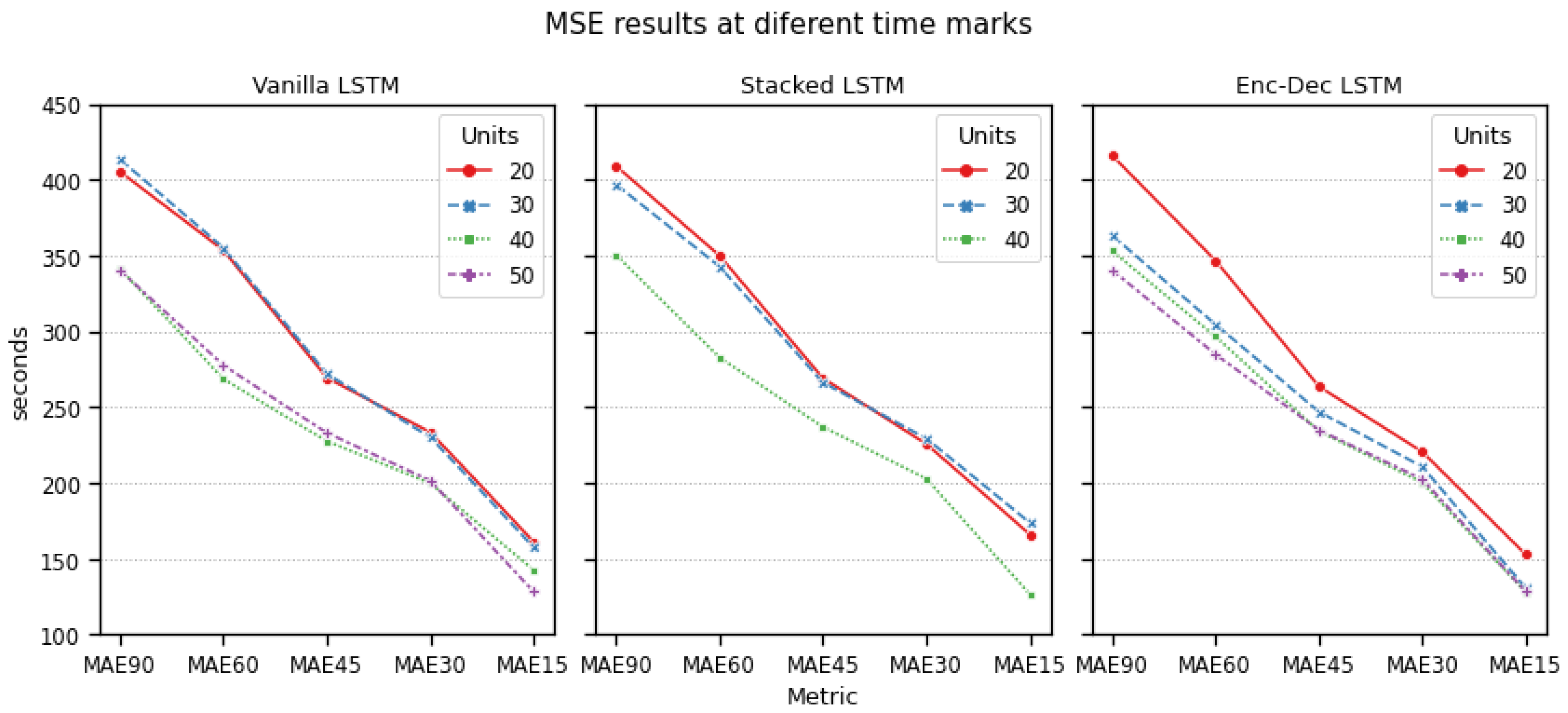
Additionally, we calculate MAE at different milestones along the trajectory: we cut the trajectory at 90, 60, 45, 30 and 15 min before arrival, and make a prediction of the RTA using the latest available vectors. Then, we average the MAE across all the flights to describe how each model performs at different time horizons.
5. Results
The experiments were executed in an Intel Core i5-1035G4 1.50GHz with 8 cores and 16 GB of RAM. All experiments were implemented using Tensorflow 2.3, Keras 2.4.3 and scikit-learn 0.24.2.
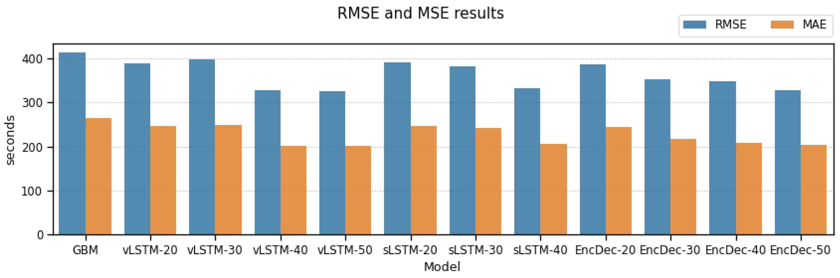
Table 2 shows RMSE and MAE values for all models included in our study, and
Figure 2 and
Figure 3 represent them at global level anf for each considered timemark, respectively.
All LSTM-based models outperform our GBM baseline model in both global MAE and RMSE values. However, this model only uses one vector to make a prediction, so LSTM models may be taking advantage of their knowing of sequences of vectors to better estimate the RTA.
At a first glance, smaller models perform worse than models with a higher number of LSTM units. This may occur because smaller sequence sizes in these models are not long enough to identify many of the relevant patterns in the input data. It might also be that the models have an insufficient capacity to correctly fit the data, and the error we are observing is due to bias error of the models themselves. However, sLSTM and Enc-Dec models, each with two layers of 20 LSTM units, do not improve the results of vLSTM albeit their higher capacity, which enforces the first hypothesis: input sequences are too short. All models increase their performance when 40 or more units are used, with a MAE lower at about 40–50 s (a 20% lower mean absolute error), and this keeps improving slightly if we increase the number of units to 50. LSTM-50 is the best model, with a MAE value of 200 s (3.33 min) versus 264 s from GBM (4.4 min) and 208.23 from EncDec-40 (3.47 min).
The results at different time marks provide similar conclusions. There exists a logical trend according to which the absolute error decreases as the end of the flight gets closer, reaching a minimum of 126.55 s 15 min before the aircraft lands. This trend is similar for all models, with vLSTM models providing more consistent results, especially at higher RTAs (between 30 and 90 min).
Of the three families of models, Vanilla LSTM reports the best results. For lower numbers of units (20 and 30 units), its performance is only slightly worse than the equivalent stacked and encoder-decoder models, even though it only has half the units. With higher numbers of units it outperforms the rest of the models, with a much lower computational cost during the training process.
6. Conclusions and Future Work
In this paper, we have proposed and evaluated different models based on LSTM neural networks to accurately estimate time of arrival using historical data. Out of the three proposed architectures, vanilla LSTM with 50 units provided the best results, with a global MAE of 200 s, and an MAE of 340 s 90 min before the flight ends, lowering to 126.55 s 15 min before landing. The length of the sequences of state vectors that are used to make the predictions is key for improving our capacity to predict ETA accurately: every architecture manifested significant improvements with sequence lengths of 40 and higher.
The data used in this paper has been generated using a data integration workflow that is currently under development. In the future, we plan to incorporate data such as weather conditions and additional flight plan data whose importance has been demonstrated in previous works to predict ETAs more accurately. We are also currently exploring the combination of different techniques, such as Convolutional Neural Networks, to help the models to extract information from specific types of data like GPS position points.


 ,
, 

