Reduction in the Estimation Error in Load Inversion Problems: Application to an Aerostructure ^†

Abstract

The present work focuses on the inverse identification of loads acting on wing-like geometries, through strain measurements. These loads are considered quasi-static and considered acting at discrete stations across the span of the wing. A demonstrative case study is investigated, focusing on a complex composite structure, an Unmanned Aerial Vehicle (UAV) fin. To achieve this, a high-fidelity Finite Element model is developed, with “virtual” strain data generated through simulations. The technical challenge of optimal sensor placement is addressed with D-optimal designs, which promise sensor networks (sensor locations and strain components) that produce minimal uncertainty propagation from strain measurements to load estimates. These designs are obtained through the implementation of Genetic Algorithms. Different sensor networks with an increasing number of sensors are evaluated in order to identify a further reduction in epistemic uncertainty posed by the problem’s ill-conditioned nature.

1. Introduction

Aircraft face harsh and unpredictable conditions that necessitate continuous monitoring of their structural integrity. Structural health monitoring (SHM) enhances safety and operational efficiency by reducing maintenance downtime and supporting airworthiness certification. Accurate load identification, the focus of this study, aims to reconstruct loads from measurable responses like strain and displacement. Knowing true load histories allows for precise fatigue calculations, enabling a shift from preventive to condition-based maintenance. Load identification is an inverse, ill-posed problem sensitive to errors from sensor noise, modeling inaccuracies, and environmental factors, which can significantly affect reliability.

In load monitoring approaches, as outlined in [1], there are two primary methodologies: training-based and training-free. Training-based methods heavily rely on machine learning (ML) techniques, utilizing datasets—either real or simulated—from various scenarios to predict flight maneuvers or establish mathematical models correlating input parameters, such as strains, stresses, or forces at discrete positions, to load estimates. Artificial neural networks (ANNs) [2] and Gaussian process (GP) regression models are commonly employed for this purpose [3]. ANNs and GP regression models necessitate a training dataset for effective operation, which impacts the accuracy and reliability of load estimates produced by these models.

Physics-based techniques, on the other hand, require smaller or zero experimental training datasets, since they rely mainly on a physical model of the structure to estimate the loading condition based on some physical input parameter. Some of these methods [4,5,6] involve the structure’s modal response to link the discrete strain measurements to the strain estimation in predetermined positions within the components; however, when the mode shapes of the structure are closely spaced, difficulties in strain prediction arise, thus limiting their applications. Other methods, like the Inverse Finite Element Method (iFEM) [7,8,9], aim at reconstructing the full displacement, and thus, strain fields of the structure based on a minimization of the error functional between the discrete strain measurements and a numerical formulation of the same without requiring any knowledge beforehand on boundary conditions and material properties of the structure.

Another method [1,9,10,11,12] for load identification, sometimes referred as conversion or the influence matrix approach, reconstructs a set of loads by minimizing an error functional comparing discrete strain measurements with a numerical estimation of the same as a function of the unknown loads. Once the conversion matrix connecting the strain measurements in specific locations to the equivalent load set representative of the real load condition based on the FEM of the structure is computed, the full strain field can be estimated exploiting an inverse-direct approach. Indeed, after the equivalent load set is determined using a least squares approach, the reconstruction of the full strain field becomes feasible through straightforward matrix–vector multiplication. This ensures real-time functionality with a reduced computational workload.

2. Theoretical Background

2.1. Mathematical Formulation for the Conversion Matrix Approach

The methodology followed is based on the Sensitivity Response Method. Its numerical implementation was first introduced by Wickham et al. [13]. Intrinsic to this method are the following assumptions:

• The applied loads do not lead to non-linear response of the structure; the material response remains within its elastic regime, and thus, superposition can be applied.
• The structure is loaded at a finite number of known locations. The loading direction is also given, leaving their magnitude as the sole unknown variable for evaluation.
• The imposed loads are static or quasi-static, making inertia effects negligible.

Suppose a structure is subjected to an unknown and arbitrary load, L_u. The structure deforms, resulting in a strain field ε_u function of the load L_u itself. Consider that the structure is instrumented with n_s sensors measuring the deformation at x_s discrete points. The measures at the time instant t are collected in a n_s × 1 vector ε.

$$\mathit{\epsilon }=\left\{\begin{array}{c}{\mathit{\epsilon }}_{\mathbf{1}}\\ ⋮\\ {\mathit{\epsilon }}_{\mathit{n}\mathit{s}}\end{array}\right\}$$

(1)

The external loads, expressed as a series of n_rl discrete real loads or a simplified equivalent representative version, are computed through a least squares approach by minimizing the error e, as a function of the load (or equivalent load) set, F.

$$\mathit{e}\left(\mathit{F}\right)={({\mathit{\epsilon }}^{\mathit{m}}-{\mathit{\epsilon }}^{\mathit{n}}(\mathit{F}\left)\right) }^{\mathbf{2}}={({\mathit{\epsilon }}^{\mathit{m}}-{\mathit{\epsilon }}^{\mathit{n}}(\mathit{F}\left)\right) }^{\mathit{T}} \left({\mathit{\epsilon }}^{\mathit{m}}-{\mathit{\epsilon }}^{\mathit{n}}\left(\mathit{F}\right)\right)$$

(2)

Assuming linear-elastic behavior of the structure, the i^th strain measurement ε_i in the vector εⁿ can be written as

$${\mathit{\epsilon }}_{\mathit{i}}={\mathit{\epsilon }}_{\mathit{i}}^{\mathbf{1}}+{\mathit{\epsilon }}_{\mathit{i}}^{\mathbf{2}}+\cdots +{\mathit{\epsilon }}_{\mathit{i}}^{{\mathit{n}}_{\mathit{r}\mathit{l}}}=\sum _{\mathit{j}=\mathbf{1}}^{{\mathit{n}}_{\mathit{r}\mathit{l}}}{\mathit{\epsilon }}_{\mathit{i}}^{\mathit{j}}$$

(3)

where ${\epsilon }_i^j$ is the strain in the position x_i when only the j^th load is acting on the structure.

• Furthermore, assuming a linear relationship between load and strain such that

  $${\mathit{\epsilon }}^{\mathit{n}}\left(\mathit{t}\right)=\sum _{\mathit{j}=\mathbf{1}}^{{\mathit{n}}_{\mathit{l}\mathit{r}}}{\mathit{\epsilon }}^{\mathit{j}}\left(\mathit{t}\right)=\sum _{\mathit{j}=\mathbf{1}}^{{\mathit{n}}_{\mathit{l}\mathit{r}}}{\mathit{a}}^{\mathit{j}}{\mathit{F}}_{\mathit{j}}\left(\mathit{t}\right)=\mathit{A}\mathit{F}\left(\mathit{t}\right)$$

  (4)

  in which the α_ij term is the strain–force proportionality factor, often referred to as “influence” or “calibration “coefficient. Additionally, F is a 1 × n_lr vector containing all the load aiming to reconstruct, and A is the n_s × n_l “conversion matrix” containing the influence coefficients between the strain and the loads.

$$\mathit{A}=\left[\begin{array}{ccc}{\mathit{\alpha }}_{\mathbf{11}}& \dots & {\mathit{\alpha }}_{\mathbf{1}\mathit{n}\mathit{l}}\\ ⋮& \ddots & ⋮\\ {\mathit{\alpha }}_{\mathit{n}\mathit{s}\mathbf{1}}& \dots & {\mathit{\alpha }}_{\mathit{n}\mathit{s}\mathit{n}\mathit{l}}\end{array}\right]$$

(5)

Each α_ij component of the α matrix can be interpreted as the strain in the position x_i that one reads if a single unitary force j is acting on the structure.

Substituting Equation (4) into (2) yields

$$\mathit{e}\left(\mathit{F}\right)={\left({\mathit{\epsilon }}^{\mathit{m}}-\mathit{A}\mathit{F}\right) }^{\mathbf{2}}={\left({\mathit{\epsilon }}^{\mathit{m}}-\mathit{A}\mathit{F}\right)}^{\mathit{T}} \left({\mathit{\epsilon }}^{\mathit{m}}-\mathit{A}\mathit{F}\right)={\mathit{\epsilon }}^{\mathit{m}\mathit{T}}{\mathit{\epsilon }}^{\mathit{m}}-{\mathit{\epsilon }}^{\mathit{m}\mathit{T}}\mathit{A}\mathit{F}-{\mathit{F}}^{\mathit{T}}{\mathit{A}}^{\mathit{T}}{\mathit{\epsilon }}^{\mathit{m}}+{\mathit{F}}^{\mathit{T}}{\mathit{A}}^{\mathit{T}}\mathit{A}\mathit{F}$$

(6)

Lastly, by minimizing the error with respect to the unknown load F ($\frac{\mathsf{\partial }e}{\mathsf{\partial }F}=0$), we have the solution of the inverse problem:

$$\mathit{F}={\left({\mathit{A}}^{\mathit{T}}\mathit{A}\right)}^{-\mathbf{1}}{\mathit{A}}^{\mathit{T}}{\mathit{\epsilon }}^{\mathit{m}}={\mathit{A}}^{+}{\mathit{\epsilon }}^{\mathit{m}}$$

(7)

where $A^{+}$ is the pseudoinverse matrix of the conversion matrix A. Note that for the inverse problem to be solvable, one has to verify that the matrix A^TA is invertible, resulting in the requirement that the number of sensors must at least match the number of loads, and they must be positioned so each load yields distinct information—meaning the columns of the conversion matrix are linearly independent.

2.2. Optimal Experimental Designs—D-Optimality

Load identification through strain sensing is an ill-conditioned inverse problem. Optimal sensor placement is key in structural health monitoring, maximizing data value while minimizing sensor count. A forward predictive model—analytical, Finite Element, or statistical—is needed to relate measured strains to load estimates. The topology of sensor placement results in a different representation of the forward predictive model and thus the inverse. Therefore, sensor placement can be defined deliberately so that the ill conditioning of the problem is minimized. For this purpose, the D-optimality criterion is employed along with a genetic algorithm for the optimization of the sensor placement [14]. The D-optimality criterion, which is used for parameter estimation, can serve as a promising criterion in deciding/guiding the optimal sensor placement locations [15,16,17].

The expression for the load estimates after the least squares solution of the inverse problem is

$$\mathit{F}={\left({\mathit{A}}^{\mathit{T}}\mathit{A}\right)}^{-\mathbf{1}}{\mathit{A}}^{\mathit{T}}{\mathit{\epsilon }}^{\mathit{m}}+\mathit{e}={\mathit{A}}^{+}{\mathit{\epsilon }}^{\mathit{m}}+\mathit{e}$$

(8)

Given that ${\left(A^{T}A\right)}^{-1}$ exists, the covariance matrix for the load estimates is defined as

$$\mathbf{v}\mathbf{a}\mathbf{r}\left(\mathit{F}\right)=\mathbf{v}\mathbf{a}\mathbf{r}\left(\mathit{\epsilon }\right){\left({\mathit{A}}^{\mathit{T}}\mathit{A}\right)}^{-\mathbf{1}}={\mathit{\sigma }}^{\mathbf{2}}{\left({\mathit{A}}^{\mathit{T}}\mathit{A}\right)}^{-\mathbf{1}}$$

(9)

where the diagonal terms of the covariance matrix of F correspond to the variance of each individual load estimate, while each of the off-diagonal terms is the covariance between the load estimates F_k and F_l for k ≠ l. The matrix ${\left(A^{T}A\right)}^{-1}$ is referred to as the sensitivity matrix of A (inverse of the fisher information matrix), and for a given variance in strain measurements, σ², its minimization can essentially increase the precision of the load estimations. Matrix A, and therefore its sensitivity matrix ${\left(A^{T}A\right)}^{-1}$, depends on the locations and angular orientations of the strain sensors attached to the structure. Hence, the optimal sensor placement is the one that minimizes the error between the predicted loads and strain measurements, which essentially corresponds to the minimization of the sensitivity matrix of A. Let the information related to the number of sensors (n), topology (x_n, y_n, z_n), and strain component (ε_x, ε_y, ε_xy) be collected in a parameter vector θ, then

$$\mathit{\theta }={\left\{\mathit{n},(x_n, y_n, z_n),(\mathbf{s}\mathbf{t}\mathbf{r}\mathbf{a}\mathbf{i}\mathbf{n} \mathbf{c}\mathbf{o}\mathbf{m}\mathbf{p}\mathbf{o}\mathbf{n}\mathbf{e}\mathbf{n}\mathbf{t})\right\}}^{\mathit{T}}$$

(10)

According to the D-optimal criterion where ‘D’ represents the determinant, the goal is to find the matrix A that minimizes the quantity:

$$\mathbf{d}\mathbf{e}\mathbf{t}\left|{\left({\mathit{A}}^{\mathit{T}}\mathit{A}\right)}^{-\mathbf{1}}\right|$$

(11)

This is equivalent to maximizing the determinant of the Fisher information matrix $\mathrm{d}\mathrm{e}\mathrm{t}\left|A^{T}A\right|$, and such a design is called the D-optimal design [17], thus,

$${\mathsf{\Theta }}_{\mathbf{D}-\mathbf{o}\mathbf{p}\mathbf{t}\mathbf{i}\mathbf{m}\mathbf{a}\mathbf{l}}={\mathbf{a}\mathbf{r}\mathbf{g}\mathbf{m}\mathbf{a}\mathbf{x}}_{\mathit{\theta }}(\mathbf{det}\left|{(\mathit{A}}^{\mathit{{\rm T}}}\left(\mathit{\theta }\right)\mathit{A}\left(\mathit{\theta }\right)\right|)$$

(12)

2.3. Genetic Algorithms

Genetic algorithms (GA) are evolutionary optimization tools well-suited for engineering and scientific problems. They efficiently search complex, multidimensional spaces—handling nonlinearity and local optima better than traditional methods—by evolving a population of solutions using selection, crossover, and mutation. Unlike gradient-based approaches, they work without requiring differentiable or convex functions and avoid being trapped in local optima [18].

2.4. Optimal Sensor Placement (OSP) Design Framework

The proposed OSP process occurs in two stages. First, Finite Element analysis generates strain–load correlation data by simulating unit calibration loads. This data forms the basis for the conversion matrix A, linking possible strain sensors to loads. Within the optimization, the GA sets the sensor number and design constraints (e.g., locations, strain components). It then searches for high-fitness solutions based on the D-optimality criterion (Equation (12)) over a fixed number of generations. For each design vector θ, the corresponding A matrix is retrieved, and its fitness is evaluated, eventually providing the θ_D-optimal and its corresponding conversion matrix A_D-optimal.

3. Numerical Analysis and Results

3.1. Model Developement

In the present case study, a UAV fin is examined, Figure 1. The fin has a span of 1276 mm, a root chord of 476.1 mm, and a tip chord of 278.7 mm. It consists of the upper and lower skins, front and rear spar, and two ribs. It is made from composite materials, specifically carbon fiber (unidirectional and woven plies) and aramid honeycomb core. A complete overview of material properties is given in Table 1.

Figure 1. (a) Finite Element model with optimal sensor locations. (b,c) Thickness plots.

Table 1. Lay-up of Fin’s structural parts.

STRUCTURAL PART	LAY-UP	TOTAL THICKNESS
LOWER AND UPPER SKINS	45w/0_core/45w	3.44 mm
LOWER AND UPPER SPAR CAPS	45w/45w/0_core/45w/45w/0/0/45w/0/0/45w	4.92 mm
FRONT SPAR WEB	45w/45w/45w/45w	0.87 mm
REAR SPAR WEB	45w/45w/0_core/45w/45w	3.87 mm
RIBS	45w/45w	0.44 mm

For the discretization of the UAV fin, PATRAN/NASTRAN 2008 r1 software is mostly used with four node shell elements (QUAD4), along with a limited number of triangular elements (CST), for better adaptation to the structure’s shape. The average mesh size is 18 mm, as it provided sufficiently accurate results while maintaining reasonable computational time. The fin is clamped at the spar root to simulate realistic support constraints. Loads are applied at a specific station near the tip using an RB2 Multi-Point Constraint (MPC) element. To achieve this, all peripheral nodes at the free end (tip station) are kinematically coupled to a single master node located at the aerodynamic center of the foil section. This master node serves as the load application point. An indicative deformation plot is shown below in Figure 2.

Figure 2. Indicative deformation plot.

The Genetic Algorithm (GA) starts with 100 random chromosomes, each representing a sensor layout. Fitness is evaluated using D-optimality; crossover and mutation probabilities are 0.8 and 0.15, respectively. Tournament selection (groups of five), along with Hall of Fame elitism, ensures diversity while retaining the best solution. The algorithm runs for 15,000–20,000 generations, with larger sensor networks requiring more iterations for convergence due to the increased search space.

3.2. Results

In Figure 1a, the optimal sensor locations are also illustrated (red circles). The GA OSP procedure performed well by placing most sensors close to the support region of the structure and a few positioned close to the load application point in alignment with areas where higher strains are anticipated. It is notable that the algorithm selected sensors from multiple structural components including the upper and lower skin, as well as front and rear spar despite their material heterogeneity. This placement strategy highlights the robustness of the optimization procedure in adapting to complex geometries and varying material properties. With the optimal sensor placement established, the next step involves the reconstruction of the applied loads based on noise-polluted measurements. Vector ${\mathit{\epsilon }}^{\mathit{m}}$ polluted with White Gaussian Noise of 5μ and several load cases are explored after the D-optimal conversion matrix is established for six loads acting on the fin tip. In the following load case, the target loads aiming to identify are forces F < 1.5, 1.5, 2.5 > kN and moments M < −2, −2, −2 > kNm acting along the x, y, and z axes, respectively. In Figure 3, the histogram of the identified loads with twelve-sensor networks is illustrated, estimated by 10,000 Monte Carlo simulations. Afterwards, the results of the mean identified loads and Coefficient of Variation for different sensor networks are recorded in Table 2.

Figure 3. Distribution of identified load component Mx- 12 sensors grid.

Table 2. Mean and CoV of identified loads for different number of sensors from 10000 MC simulation.

# SENSORS		LOAD 1 (FX)	LOAD 2 (FY)	LOAD 3 (FZ)	LOAD 4 (MX)	LOAD 5 (MY)	LOAD 6 (MZ)
6	mean	1.4999348	1.49999188	2.49999928	−1.9999493	−1.999978	−2.0001056
	CoV	1.223113	0.1034149	0.0293033	0.2734192	0.3467196	0.6844731
12	mean	1.500077	1.4999963	2.5000048	−2.000012	−2.000012	−2.000011
	CoV	0.803082	0.094592	0.0177268	0.2346718	0.2035107	0.5733383
24	mean	1.50006	1.5000135	2.4999969	−1.9999992	−1.999947	−1.9998506
	CoV	0.596135	0.06899981	0.0137325	0.1409092	0.1572164	0.4216038
48	mean	1.49999	1.50000163	2.499997	−2.0000308	−1.999988	−2.0000135
	CoV	0.455827	0.05536822	0.0102288	0.1018635	0.1104922	0.3151355

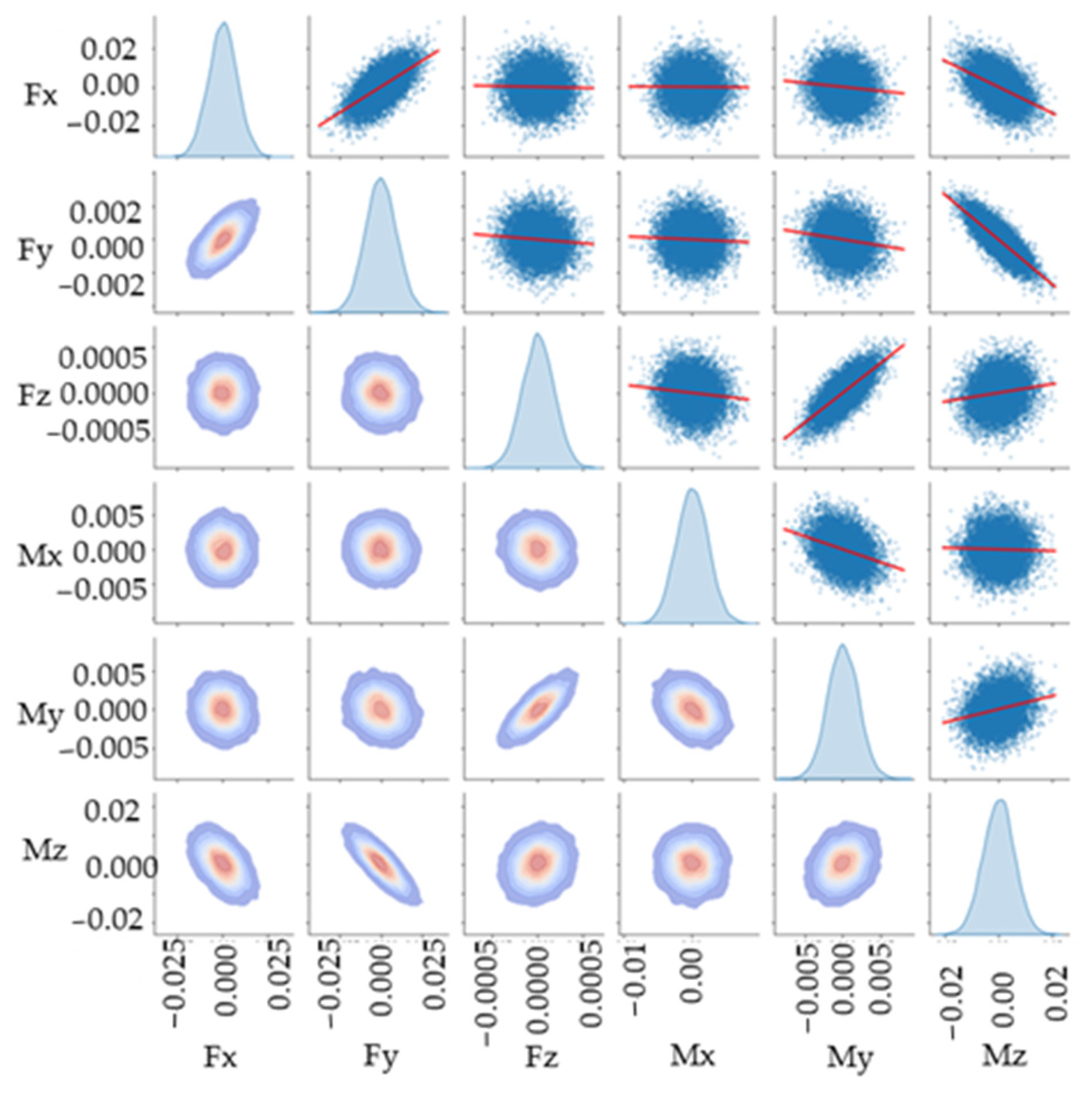
The results indicate that the identified loads closely follow a normal distribution centered around the targeted load values, with minimal bias. The standard deviations are relatively small, indicating that the load identification is stable. This pair plot, Figure 4, visualizes the distribution of the error in the load identification for each load in the diagonal and the correlations between different load components. Overall, there is either no or weak correlation between the load components, and the spread of errors is small, highlighting the effectiveness of the optimal sensor placement. Load 3 (shear force-Fz) and load 5 (bending moment) show linear correlation, which makes sense physically, since a shear force acting on the fin tip will create a bending moment distribution, influencing the structural response similarly.

Figure 4. Pair plot of the error model in the load identification problem of the fin—12 sensors grid, 10,000 Monte Carlo simulations.

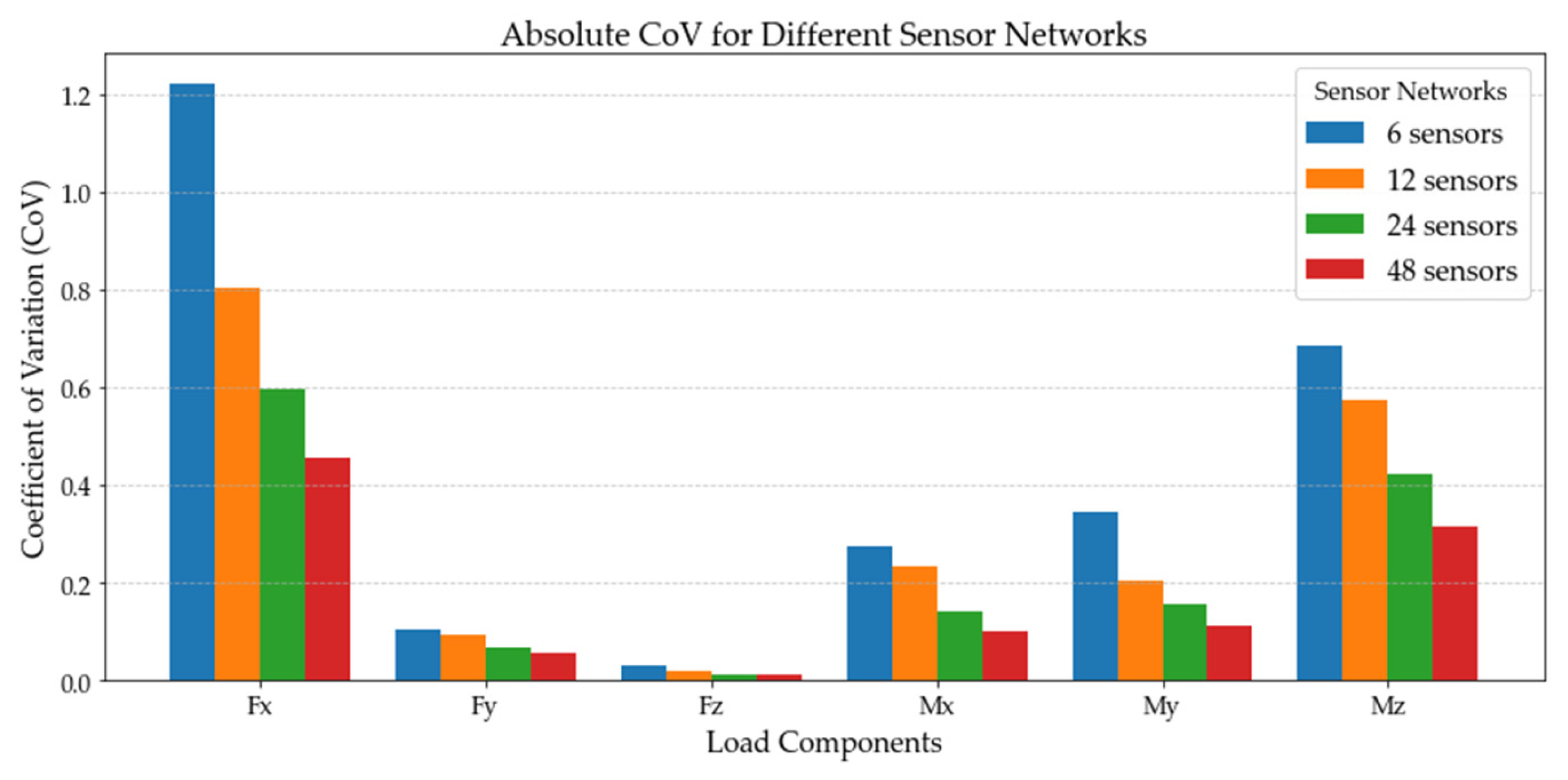
The following bar plot (Figure 5) illustrates the Coefficient of Variation (CoV) across load components for sensor networks of 6, 12, 24, and 48.

Figure 5. Values of Coefficient of Variation for each load for different sensor networks.

From the bar plot, it is obvious that increasing the number of sensors significantly reduces the CoV, suggesting that denser sensor networks improve accuracy of the estimated loads while reducing the variance of errors.

4. Conclusions

The study confirmed that optimal sensor placement plays a crucial role in minimizing load identification errors. The integration of D-optimality criterion through genetic algorithms effectively recognized sensor locations and configurations that maximize information gain, ensuring minimal uncertainty in the reconstructed loads. The genetic algorithm sensor placement optimization demonstrated adaptability even in complex design spaces like the UAV fin structure, which consists of several components with varying material properties.

The conversion matrix approach successfully estimated applied loads accurately and consistently despite the presence of noise in strain measurements. Monte Carlo simulations were performed, validating the normality and homogeneity assumption in the load identification, as promised by the White Gaussian Noise model. The pair plots confirmed that the error model is unbiased, exhibiting weak statistical correlation between different load components. Furthermore, analytically derived variances for the estimated loads closely match the Monte Carlo results, further validating the error model assumptions.

Additionally, increasing the number of sensors systematically reduced the uncertainty in load estimations, as reflected by the decreasing Coefficient of Variation. Loads such as shear force (Fz), twisting moment-torque (Mx), and bending moment (My) were identified with high precision, while axial force (Fx) exhibited higher variance, likely due to its weaker strain response in the measured data.

References

1. Colombo, L.; Sbarufatti, C.; Bosco, L.D.; Bortolotti, D.; Dziendzikowski, M.; Dragan, K.; Concli, F.; Giglio, M. Numerical and experimental verification of an inverse-direct approach for load and strain monitoring in aeronautical structures. Struct. Control Health Monit. 2021, 28, e2657. [Google Scholar] [CrossRef]
2. Wada, D.; Sugimoto, Y.; Murayama, H.; Igawa, H.; Nakamura, T. Investigation of Inverse Analysis and Neural Network Approaches for Identifying Distributed Load using Distributed Strains. Trans. Jpn. Soc. Aeronaut. Space Sci. 2019, 62, 151–161. [Google Scholar] [CrossRef]
3. Fuentes, R.; Cross, E.; Halfpenny, A.; Worden, K.; Barthorpe, R.J. Aircraft Parametric Structural Load Monitoring Using Gaussian Process Regression. 2014. Available online: https://inria.hal.science/hal-01022048 (accessed on 29 November 2024).
4. He, J.; Zhou, Y.; Guan, X.; Zhang, W.; Zhang, W.; Liu, Y. Time Domain Strain/Stress Reconstruction Based on Empirical Mode Decomposition: Numerical Study and Experimental Validation. Sensors 2016, 16, 1290. [Google Scholar] [CrossRef] [PubMed]
5. He, J.; Zhou, Y.; Guan, X.; Zhang, W.; Wang, Y.; Zhang, W. An Integrated Health Monitoring Method for Structural Fatigue Life Evaluation Using Limited Sensor Data. Materials 2016, 9, 894. [Google Scholar] [CrossRef] [PubMed]
6. Sireta, F.-X.; Storhaug, G. A Modal Approach for Holistic Hull Structure Monitoring from Strain Gauges Measurements and Structural Analysis. In Proceedings of the Off-Shore Technology Conference, Houston, TA, USA, 2–5 May 2022. [Google Scholar] [CrossRef]
7. Oboe, D.; Colombo, L.; Sbarufatti, C.; Giglio, M. Shape Sensing of a Complex Aeronautical Structure with Inverse Finite Element Method. Sensors 2021, 21, 1388. [Google Scholar] [CrossRef] [PubMed]
8. Gherlone, M.; Cerracchio, P.; Mattone, M.; Di Sciuva, M.; Tessler, A. Shape sensing of 3D frame structures using an inverse Finite Element Method. Int. J. Solids Struct. 2012, 49, 3100–3112. [Google Scholar] [CrossRef]
9. Esposito, M.; Mattone, M.; Gherlone, M. Experimental Shape Sensing and Load Identification on a Stiffened Panel: A Comparative Study. Sensors 2022, 22, 1064. [Google Scholar] [CrossRef] [PubMed]
10. Nakamura, T.; Igawa, H.; Kanda, A. Inverse identification of continuously distributed loads using strain data. Aerosp. Sci. Technol. 2012, 23, 75–84. [Google Scholar] [CrossRef]
11. Colombo, L.; Sbarufatti, C.; Zielinski, W.; Dragan, K.; Giglio, M. Numerical and experimental flight verifications of a calibration matrix approach for load monitoring and temperature reconstruction and compensation. Aerosp. Sci. Technol. 2021, 118, 107074. [Google Scholar] [CrossRef]
12. Panagiotopoulos, S.; Anyfantis, K.N. Load identification for fatigue life assessment in ship hull structural elements. In Proceedings of the 10th European Workshop on Structural Health Monitoring (EWSHM 2024), Potsdam, Germany, 10–13 June 2024. [Google Scholar] [CrossRef]
13. Wickham, M.J.; Riley, D.R.; Nachtsheim, C.J. Integrating Optimal Experimental Design into the Design of a Multi-Axis Load Transducer. J. Manuf. Sci. Eng. 1995, 117, 400–405. [Google Scholar] [CrossRef]
14. Gupta, D.K.; Dhingra, A.K. Input load identification from optimally placed strain gages using D-optimal design and model reduction. Mech. Syst. Signal Process. 2013, 40, 556–570. [Google Scholar] [CrossRef]
15. Wang, J.; Law, S.; Yang, Q. Sensor placement methods for an improved force identification in state space. Mech. Syst. Signal Process. 2013, 41, 254–267. [Google Scholar] [CrossRef]
16. Wang, Y.; Zhou, Z.; Xu, H.; Li, S.; Wu, Z. Inverse Load Identification in Stiffened Plate Structure Based on in situ Strain Measurement. Struct. Durab. Health Monit. 2021, 15, 85–101. [Google Scholar] [CrossRef]
17. Galil, Z.; Kiefer, J. Time- and Space-Saving Computer Methods, Related to Mitchell’s DETMAX, for Finding D-Optimum Designs. Technometrics 1980, 22, 301–313. [Google Scholar] [CrossRef]
18. Goldberg, D.E. Genetic Algorithms in Search, Optimization and Machine Learning; Addison-Wesley Publishing Company, Inc.: Carrollton, TX, USA, 1989. [Google Scholar]
Disclaimer/Publisher’s Note: The statements, opinions and data contained in all publications are solely those of the individual author(s) and contributor(s) and not of MDPI and/or the editor(s). MDPI and/or the editor(s) disclaim responsibility for any injury to people or property resulting from any ideas, methods, instructions or products referred to in the content.
Article Metrics
Citations
Article Access Statistics
Multiple requests from the same IP address are counted as one view.