Robust IMU Sensor Fusion via Schreiber’s Nonlinear Filtering Approach ^†

Abstract

This study introduces a hybrid sensor fusion approach that integrates Schreiber’s nonlinear filter with traditional filtering methods to enhance the performance of IMU-based systems in autonomous vehicles. As autonomous vehicles grow more dependent on Inertial Measurement Unit (IMU) data for real-time stability and control, the need for resilient and accurate sensor fusion becomes critical. This research addresses that need by introducing a method capable of maintaining robustness under highly dynamic and uncertain conditions. Accelerometer and gyroscope data from an IMU are first fused using a complementary filter. The fused signals are then refined by phase-space reconstruction and local manifold projection, improving noise resilience and maintaining system dynamics. Two datasets are used to assess the methodology: one was collected indoors with a smartphone, and another was captured outdoors using a Bosch sensor in various environmental settings. The proposed method demonstrates superior noise reduction, greater resistance to outliers, and improved signal consistency compared to conventional complementary and Kalman filters. The findings demonstrate how chaos-based nonlinear filtering may improve the reliability of sensor fusion on a variety of sensing platforms in highly dynamic environments. Given the importance of IMU data for maintaining vehicle stability, this study seeks to support the development of more stable autonomous transportation systems.

1. Introduction

In the ongoing evolution of mobility, autonomous transportation systems are emerging as a cornerstone of future urban and interurban infrastructure. These systems, which range from self-driving cars to cooperative vehicle fleets, must operate in dynamic, unpredictable environments while ensuring safety, efficiency, and stability. At the heart of their decision-making and control capabilities lies sensor fusion, especially using data from Inertial Measurement Units (IMUs), which are essential for real-time estimation of vehicle orientation and motion.

However, traditional fusion methods such as the Kalman filter and complementary filter, while effective under idealized or stationary conditions, struggle to perform reliably amid nonlinearities, noise, and sudden changes typical of real-world driving. These limitations can compromise vehicle stability, a critical factor for passenger safety and system reliability in autonomous operations. To address these challenges, this study introduces a hybrid sensor fusion approach that incorporates Schreiber’s nonlinear filtering, enhancing the accuracy and robustness of IMU-based state estimation. The proposed method is particularly suited to chaotic or rapidly changing environments, where conventional filters may fail to accurately represent complex dynamic behavior.

By enhancing the resilience of sensor fusion under such conditions, the proposed approach contributes directly to improving vehicle stability and reliability in autonomous systems. Ensuring consistent performance in edge cases—such as sudden maneuvers, sensor noise spikes, or variable road conditions—is essential for building public trust and meeting safety standards. The methodology presented here provides a foundation for more dependable motion estimation in autonomous platforms and represents a step toward enhanced fault tolerance, stability, and safety in future transportation systems.

As system complexity grows and transportation advances toward higher automation and connectivity, there is a pressing need for sensor fusion methods that can adeptly handle dynamic and nonlinear environments. The field of chaos theory emerges as a promising solution, offering sophisticated tools to model systems that are inherently unpredictable. The utilization of chaotic attractors and hybrid chaos algorithms within sensor fusion frameworks allows for a more nuanced capture of signal variations, both on a granular level and across wider patterns. This enhanced capability not only bolsters the reliability of the data, but also plays a crucial role in maintaining the safety and integrity of the system.

In light of these considerations, our study introduces an innovative sensor fusion methodology that marries the strengths of nonlinear filtering with the capabilities of hybrid chaos-based algorithms. This method is specifically tailored to excel in environments characterized by uncertainty and dynamism. By fusing the theoretical underpinnings of chaos modeling with practical, real-world applications, our approach seeks to address the key limitations of modern data-driven systems. The proposed method stands to significantly elevate the accuracy and robustness of sensor fusion, ensuring that performance and safety are not compromised in an era where both are paramount.

In the subsequent sections, this paper will methodically examine the different elements of the hybrid sensor fusion approach. Section 2 offers a review of the relevant literature. Section 3 delves into the theoretical foundations of the proposed technique, elaborating on the complexities of Schreiber’s filter, the complementary filter, and the Kalman filter. Section 4 presents a unified perspective of the algorithm employed, demonstrating its integration with IMU sensor data. Section 5 assesses the proposed technique’s performance and effectiveness through the results achieved. Finally, Section 6 concludes the paper by encapsulating the principal conclusions and exploring future avenues for research that aim to further refine the application of sensor fusion technology.

2. Related Works

Chaos theory examines the behavior of dynamic systems that are highly sensitive to initial conditions. Although seemingly random, these systems follow deterministic laws and can be described by chaotic attractors, making them well-suited for modeling complex, nonlinear systems.

A key feature of chaotic systems is deterministic chaos, where small differences in initial conditions lead to vastly different outcomes, a phenomenon known as the butterfly effect. Chaotic attractors, such as the Lorenz and Rössler attractors, provide a mathematical framework for identifying structure in noisy and complex data, enabling better modeling and prediction of dynamic systems [1].

Chaos theory in engineering and data science has been shown to improve predictions, optimize control systems, and find hidden patterns in multidimensional datasets. When applied to sensor fusion, chaos theory’s capacity to simulate nonlinear, multi-scale interactions offers a novel solution to the challenges of dynamic, uncertain settings. Building on these concepts, the proposed methodology aims to enhance existing sensor fusion techniques, yielding greater accuracy and robustness in complex systems.

Reference [2] identified growing challenges in using sensor data from smart devices for product development. One significant obstacle is the absence of effective data processing methods, revealing the necessity of strong filtering strategies. This study builds on that premise by proposing a nonlinear filtering method that enhances sensor fusion reliability and enables more accurate state estimation for IMU-based applications.

Reference [3] explored the integration of wearable biosensor data into smart city and healthcare frameworks, identifying the key issues affecting prediction model accuracy, such as noise, anomalies, and real-time processing constraints. They emphasized the necessity of sophisticated filtering and fusion techniques to improve sensor data reliability. Their results lend credence to the adoption of nonlinear filtering strategies, such as Schreiber’s method, which enhance sensor fusion accuracy by lowering noise while maintaining the nonlinear characteristics of the signals.

In complex systems like biological signals, where conventional linear approaches frequently fall short, Kaplan and Schreiber showed how effective nonlinear noise reduction is. Their method reduces noise while maintaining important signal properties by projecting noisy data onto manifolds and recreating phase space with delay coordinates. It performs better on electrocardiograms (ECGs) than methods such as the Wiener filter. It preserves clinically relevant information and demonstrates the adaptability of chaos-based approaches for enhancing signal clarity in irregular systems [4].

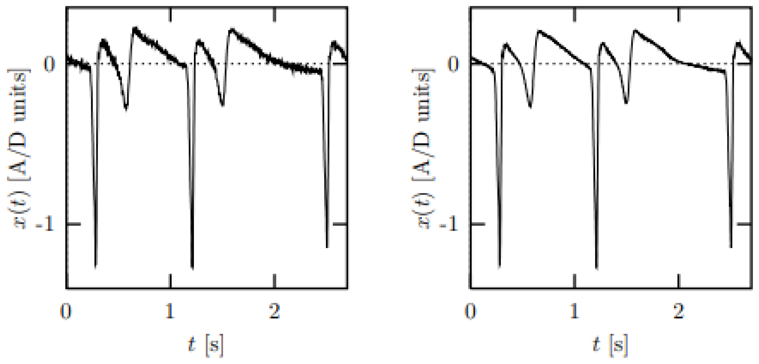
Schreiber and Kantz extended nonlinear noise reduction methods for real-time application through locally linear phase-space projections. Their approach, adaptable to both deterministic and non-deterministic systems, leverages geometric features in phase space and computational improvements for the continuous monitoring of datasets like FECGs and MCGs. By focusing on local neighborhoods, their method bridges the gap between chaos-based theory and real-world applications, remaining robust to noise fluctuations and dynamic conditions (Figure 1) [5].

Figure 1. Results of nonlinear filtering of an MCG time series [5].

Ref. [6] introduced a probabilistic approach to nonlinear noise reduction, distinguishing between state and orbit estimation for the precise reconstruction of chaotic signals. Their method effectively reduces noise even when its spectral properties overlap with the signal, a limitation of conventional linear filters. By leveraging deterministic dynamics, their technique improves the signal-to-noise ratio (SNR) and enhances the robustness of chaotic data processing, laying the groundwork for advanced sensor fusion in noisy environments.

The computational cost of such nonlinear filters must be carefully considered, particularly for real-world embedded and real-time applications. To assess whether these approaches meet the requirements of low-power resource-constrained systems, their scalability can be evaluated through complexity analysis techniques such as Landau notation [7]. Although these methods show potential to enhance signal robustness and clarity, further optimization is required to ensure low-latency performance and real-time applicability before they can be integrated into safety-critical domains such as industrial robotics and autonomous vehicles. Making nonlinear filters a practical tool for engineering work in dynamic and uncertain contexts requires overcoming these obstacles [8].

3. Methodology

This section discusses the methods employed in this study and provides a detailed overview of the techniques in the context of our use case.

3.1. Sensor Fusion

Sensor fusion is a process that combines data from multiple sensors to estimate the state of a dynamic system, resulting in an estimate that is more accurate, reliable, robust, and safer than those obtained from individual sensors. This technique involves integrating information from various sensors, such as LIDAR (Light Detection and Ranging), IMU (Inertial Measurement Unit), and ultrasonic sensors, to provide a more comprehensive understanding of a system. The fusion of these diverse sensors enhances interpretation of the environment and increases the reliability of the detection process [9].

Traditionally, systems have been standalone, with one or several sensors transmitting information to a single application. However, with a sensor fusion approach, the same tasks can be performed even in the absence of one sensor, or new applications can be added without the need for additional hardware [10].

A single sensor typically cannot supply all of the necessary information for an autonomous system to make decisions or take actions independently. Relying solely on data from a single source can significantly increase the risks associated with the operation of self-driving vehicles. Therefore, in complex environments, sensor fusion proves to be extremely beneficial, contributing to a higher degree of safety [11].

3.2. Schreiber’s Filter

Schreiber’s nonlinear filtering technique, which reconstructs the underlying system dynamics within an embedded phase space, provides a reliable method for denoising time-series data. This approach does not imply stationarity or linearity in the signal, in contrast to conventional linear or frequency-domain filters. Rather, it takes advantage of the attractor’s inherent geometric characteristics, which are a collection of states that the system tends to move toward over time, independent of initial conditions. In nonlinear dynamical systems, especially chaotic ones, the attractor often forms a low-dimensional manifold embedded in a high-dimensional observation space. By recognizing and preserving these local geometric features, Schreiber’s approach allows for more efficient noise reduction while retaining the fundamentally nonlinear properties of the underlying system. This makes it particularly suitable for applications involving complex dynamics, where traditional filters tend to distort or eliminate meaningful signal components [4].

3.2.1. Phase-Space Reconstruction

Reconstructing the system’s dynamics in a multidimensional space using delay-coordinate embedding, a technique based on Takens’ embedding theorem, constitutes the first stage of Schreiber’s nonlinear filtering methodology. When a system’s underlying structure is examined using only time series observations, particularly in situations where the governing equations are unknown or the data are noisy, this transformation is crucial [12]. Given a univariate time series $y\left(t\right)$, the reconstructed state vector $R\left(t\right)$ in an m-dimensional phase space is defined as

$$R\left(t\right)=\left[\begin{array}{ccccc}y\left(t\right),& y(t-\tau ),& y(t-2\tau ),& \dots ,& y(t-(m-1\left)\tau \right)\end{array}\right]$$

(1)

Here,

• m is the embedding dimension, determining the number of delayed observations used to construct each state vector.
• $\tau$ is the embedding delay, representing the time interval between successive components of the state vector [12].

Takens’ embedding theorem, which provides the theoretical underpinnings for reconstructing the state space of a dynamical system from a single observed time series, is the basis for this method.

Theorem 1

(Takens’ Embedding Theorem). Let M be a compact manifold of dimension d, and let $\varphi :M\to M$ be a smooth dynamical system. For a generic measurement function $h:M\to \mathbb{R}$, the delay embedding map

$${\mathsf{\Phi }}_h\left(x\right)=\left(h\left(x\right),h\left(\varphi \left(x\right)\right),h\left({\varphi }^2\left(x\right)\right),\dots ,h\left({\varphi }^{m-1}\left(x\right)\right)\right)$$

(2)

is an embedding (i.e., a diffeomorphism onto its image) if $m\ge 2d+1$.

Remark 1.

In order for the two spaces to be topologically similar under a smooth, invertible transformation, Takens’ theorem guarantees that the reconstructed state space is diffeomorphic to the original attractor.

The proof of Theorem 1 is comprehensively explained in [13]. Diffeomorphism is a smooth, invertible mapping between the two spaces that maintains the temporal evolution and trajectory structure. In practice, this ensures that no information about the dynamics of the system is lost during the reconstruction process. The manifold may stretch, bend, or rotate, but there will be no tearing or folding that would change the behavior of the system [4,14].

Example 1

(Embedding Dimension Selection). For instance, an embedding dimension of at least $m=5$ would be necessary for a system with an attractor dimension of $d=2$, according to Takens’ embedding theorem, which requires $m\ge 2d+1$.

Selecting $m=5$ ensures that the reconstructed phase space is diffeomorphic to the original attractor. This prevents the trajectories from overlapping or intersecting inappropriately, which can lead to incorrect interpretations of the system’s dynamics. As a result, the delay reconstruction effectively preserves the qualitative structure of the system and reduces the impact of observational noise, enabling more reliable analysis of the system’s behavior.

3.2.2. Local Neighborhood Identification

Finding local neighborhoods that surround each point in the embedded space is the next stage in Schreiber’s filtering method after the phase space has been reconstructed via delay embedding. To project noisy data back onto the underlying manifold, the local geometry of the attractor is estimated using these neighbors [15].

Let $R\left(t\right)\in {\mathbb{R}}^m$ denote a reconstructed state vector at time t. A local neighborhood $U\left(t\right)\subset {\mathbb{R}}^m$ is defined as the set of points that lie within a fixed Euclidean distance $\epsilon$ of $R\left(t\right)$, i.e.,

$$U\left(t\right)=\{R\left(s\right)\in {\mathbb{R}}^m\mid \parallel R\left(t\right)-R\left(s\right)\parallel <\epsilon ,s\ne t\}$$

Here, t indicates the current time index of the reference point $R\left(t\right)$, whereas s represents the time indices of other points in the reconstructed phase space. The condition $s\ne t$ ensures that the point does not include itself in its own neighborhood [16].

For nonlinear filtering applications where temporal causality must be maintained, this fixed-distance method is particularly effective since it allows for exact control over the local geometry of the rebuilt attractor. Our implementation only considers past measurements to ensure real-time applicability and prevent contamination from future data [17].

The local tangent space of the system, which approximates the geometry of the attractor around $R\left(t\right)$, is represented by the local neighborhood $U\left(t\right)$. By analyzing the shape and distribution of the points within $U\left(t\right)$, the method can infer the directions along which the system’s dynamics evolve and distinguish them from directions dominated by noise [18].

This local approximation lays the groundwork for the next step of the algorithm: projecting noisy observations onto the manifold spanned by the dominant directions in the local neighborhood, typically computed using principal component analysis (PCA) on the covariance matrix of $U\left(t\right)$.

3.2.3. Covariance Estimation and Projection

Schreiber’s method involves the determination of the local geometry of the attractor and projecting the noisy observation onto the appropriate local manifold after determining the local neighborhood U(t) around each reconstructed state vector R(t). Principal component projection and covariance analysis are carried out to accomplish this.

Let $U\left(t\right)=\{R\left(s_1\right),R\left(s_2\right),\dots ,R\left(s_k\right)\}$ be the set of k neighboring points to $R\left(t\right)$. The centroid (mean) of the neighborhood is computed as

$$s^{\left(t\right)}={\displaystyle \frac{1}{k}}\sum _{i=1}^{k}R\left(s_i\right)$$

(3)

The centered data matrix $X_t\in {\mathbb{R}}^{k\times m}$ is then formed by subtracting the centroid from each neighbor:

$$X_t(i,:)=R\left(s_i\right)-s^{\left(t\right)},\mathrm{for}i=1,\dots ,k$$

(4)

The local covariance matrix $C^{\left(t\right)}\in {\mathbb{R}}^{m\times m}$ is defined as

$$C^{\left(t\right)}={\displaystyle \frac{1}{k}}{X}_t^{\top }{X}_t$$

(5)

A collection of orthonormal eigenvectors $\{c_1,c_2,\dots ,c_m\}$ and their corresponding eigenvalues are obtained by performing an eigenvalue decomposition on $C^{\left(t\right)}$. These eigenvectors cover the local tangent space of the manifold.

To reduce the influence of noise, the original point $R\left(t\right)$ is projected onto the subspace spanned by the first Q dominant eigenvectors, typically those associated with the largest eigenvalues. The filtered point $\widehat{R}\left(t\right)$ is then computed as

$$\widehat{R}\left(t\right)=s^{\left(t\right)}+\sum _{q=1}^Q{c}_q·\left(c_q^{\top }(R\left(t\right)-s^{\left(t\right)})\right)$$

(6)

By making sure that every point is closer to the attractor while maintaining the system’s inherent dynamics, this projection step successfully lowers noise [15,19].

The final cleaned signal is obtained by averaging overlapping embedding vectors in order to rebuild the filtered time series. This approach maintains computational efficiency while adapting to non-stationary signals by dynamically updating the database of representative locations, which makes it appropriate for real-time applications.

3.3. Complementary Filter

The filter performs low-pass filtering on the low-frequency angle estimation derived from accelerometer data, while high-pass filtering is applied to the biased high-frequency angle estimation obtained through direct integration with the gyroscope output. The fusion of these two estimates yields a comprehensive estimation of the orientation. The complementary filter leverages the advantages of both the accelerometer and gyroscope. In the short term, it relies on data from the gyroscope, which is precise and unaffected by external forces. Over a longer duration, it uses accelerometer data to prevent data drift.

The low-pass filter smooths brief fluctuations by gradually accumulating changes over time. For example, if an accelerometer reading jumps to 10 degrees, the complementary filter ensures a gradual rise without spikes, depending on filter parameters and sampling rate. Meanwhile, the high-pass filter counteracts gyroscope drift by allowing for short-duration signals while filtering long-term variations, ensuring accurate angle estimation [20].

The mathematical model of the complementary filter, used to merge data from accelerometer and gyroscope sensors, is given in (7) [20]:

$${\theta }_t=\alpha \ast ({\theta }_{t-1}+{\omega }_{\mathrm{gyro}}\ast \mathsf{\Delta }t)+(1-\alpha )\ast {\beta }_{acc}$$

(7)

In this equation, ${\theta }_t$ represents the fused angle (in rad) at the current time step, which combines data from both the gyroscope and the accelerometer. The coefficient $\alpha$ is the weighting factor of the complementary filter, balancing the contribution of gyroscopic and accelerometer data. ${\omega }_{\mathrm{gyro}}$ signifies the angular velocity data (in $°/\mathrm{s}$) from the gyroscope, while ${\theta }_{t-1}$ refers to the previously estimated fused angle. ${\beta }_{acc}$ is the acceleration data (in m/s²) obtained from the accelerometer and $\mathsf{\Delta }t$ is the sampling rate. These elements collectively contribute to calculating the current estimate of the orientation.

3.4. Kalman Filter

The Kalman filter provides optimal state estimation through recursive prediction-correction cycles, minimizing the mean squared error under Gaussian noise assumptions [21]. In our orientation estimation framework, the state vector $\mathbf{x}$ represents angular position, while ${\omega }_{\mathrm{gyro}}$ (gyroscope angular velocity) serves as the process input and ${\beta }_{\mathrm{acc}}$ (accelerometer-derived angle) Sas the measurement. The prediction phase, which is also referred to as the a priori estimate, can be expressed as shown in Equation (9) [21]:

$$\begin{array}{cc}\hfill {\widehat{x}}_k^{-}& ={\widehat{x}}_{k-1}+{\omega }_{\mathrm{gyro}}\ast \mathsf{\Delta }t(\mathrm{State}\mathrm{extrapolation})\hfill \end{array}$$

(8)

$$\begin{array}{cc}\hfill P_k^{-}& =P_{k-1}+Q(\mathrm{Error}\mathrm{covariance}\mathrm{propagation})\hfill \end{array}$$

(9)

where ${\omega }_{\mathrm{gyro}}$ is gyroscope angular velocity ($°/\mathrm{s}$), Q is process noise covariance (model uncertainty, ${\mathrm{deg}}^2$), and $\mathsf{\Delta }t$ is the sampling interval (s).

The update phase (also known as the a posteriori estimate) can be formulated as shown in Equation (12) [21]:

$$\begin{array}{cc}\hfill K_k& ={\displaystyle \frac{P_k^{-}}{P_k^{-}+R}}(\mathrm{Kalman}\mathrm{gain})\hfill \end{array}$$

(10)

$$\begin{array}{cc}\hfill {\widehat{x}}_k& ={\widehat{x}}_k^{-}+K_k({\beta }_{\mathrm{accel}}-{\widehat{x}}_k^{-})(\mathrm{State}\mathrm{correction})\hfill \end{array}$$

(11)

$$\begin{array}{cc}\hfill P_k& =(1-K_k)P_k^{-}(\mathrm{Covariance}\mathrm{update})\hfill \end{array}$$

(12)

where ${\beta }_{\mathrm{acc}}$ is accelerometer-derived angle (°) and R is measurement noise covariance (sensor uncertainty, ${\mathrm{deg}}^2$).

The accelerometer-derived angle ${\beta }_{\mathrm{acc}}$ is computed from triaxial measurements:

$${\beta }_{\mathrm{acc}}={tan}^{-1}\left({\displaystyle \frac{a_y}{\sqrt{a_x^2+a_z^2}}}\right)(\mathrm{Pitch}\mathrm{angle})$$

(13)

where $a_x$, $a_y$, and $a_z$ are the accelerometer axes aligned with the sensor’s coordinate frame.

4. Proposed Hybrid Approach

Building on previous work in low-dimensional attractor analysis for traffic node reliability [22], this study extends nonlinear methods to sensor fusion. By integrating Schreiber’s nonlinear filtering with Kalman and complementary filters, the approach improves state estimation by reducing noise while preserving system dynamics. Using delay-coordinate embedding and local manifold projections, it enhances movement direction and velocity estimates, ensuring robustness against noise and outliers in dynamic environments.

Delay-coordinate embedding is used to embed the time series data from the outputs of the Complementary and Kalman filters into a reconstructed phase space.

Following this process, the phase space is reconstructed as follows:

$$R_{\mathrm{Comp}}\left(t\right)=\left[x_{\mathrm{Comp}}\left(t\right),x_{\mathrm{Comp}}(t-\tau ),\dots ,x_{\mathrm{Comp}}(t-(m-1)\tau )\right]$$

(14)

and for those of Kalman filter:

$$R_{\mathrm{Kal}}\left(t\right)=\left[x_{\mathrm{Kal}}\left(t\right),x_{\mathrm{Kal}}(t-\tau ),\dots ,x_{\mathrm{Kal}}(t-(m-1)\tau )\right]$$

(15)

where m is the embedding dimension, $\tau$ is the delay, and $x_{\mathrm{comp}}\left(t\right)$ and $x_{\mathrm{Kal}}\left(t\right)$ are the outputs of the Complementary and Kalman filters at time t (Equation (3)). The ideal delay $\tau$ is found using well-established techniques like mutual information or autocorrelation, guaranteeing that the reconstructed dynamics unfold without overlapping trajectories. Takens’ Embedding Theorem is applied to determine the embedding dimension m (Theorem 1).

To cut down on noise, Schreiber’s filter is applied independently to each filter’s output following phase-space reconstruction. Each point $R_{\mathrm{comp}}\left(t\right)$ in the reconstructed phase space, derived from the complementary filter output, is processed by finding a local neighborhood $U_{\mathrm{comp}}\left(n\right)$ within a given distance $ϵ$, which is restricted to temporally preceding points to preserve causality. Similarly, for the Kalman filter output, each point $R_{\mathrm{Kal}}\left(t\right)$ has a local neighborhood $U_{\mathrm{Kal}}\left(n\right)$ around it. Covariance matrices capture the primary directions in the local phase space derived from the accelerometer and gyroscope-based trajectories, respectively.

Thus, Equation (6) can be applied to the outputs of both filters as follows:

$${\widehat{R}}_{\mathrm{comp}}\left(t\right)=s_{\mathrm{comp}}^{\left(t\right)}+\sum _{q=1}^Q{c}_{\mathrm{comp},q}·\left(c_{\mathrm{comp},q}^{\top }(R_{\mathrm{comp}}\left(t\right)-s_{\mathrm{comp}}^{\left(t\right)})\right)$$

(16)

$${\widehat{R}}_{\mathrm{Kal}}\left(t\right)=s_{\mathrm{Kal}}^{\left(t\right)}+\sum _{q=1}^Q{c}_{\mathrm{Kal},q}·\left(c_{\mathrm{Kal},q}^{\top }(R_{\mathrm{Kal}}\left(t\right)-s_{\mathrm{Kal}}^{\left(t\right)})\right)$$

(17)

The corrected centers of mass for the accelerometer and gyroscope regions are represented by $s_{\mathrm{comp}}^{\left(t\right)}$ and $s_{\mathrm{Kal}}^{\left(t\right)}$ in this case, and Q is the number of eigenvectors used to approximate the structure of the local manifold. This procedure effectively reduces noise while preserving the underlying dynamics of the signals.

To sum up, the sequence of the filtering operations in the hybrid approach is shown below:

• First, the Complementary and Kalman filters process the raw sensor input, producing two separate estimates of the system state.
• To prepare the data for nonlinear analysis, each filtered signal is embedded into a higher-dimensional phase space using delay-coordinate embedding.
• To capture the geometry of the dynamics of the system, a local neighborhood is identified using a fixed distance criterion for each point in the reconstructed space.
• Each neighborhood’s local covariance matrix is calculated, and dominant directions of local variation (tangent space) are estimated using Principal Component Analysis (PCA).
• In order to minimize noise and preserve key dynamical structure, the original reconstructed point is projected onto the locally estimated manifold.

5. Results and Discussion

In Section 5, the initial step involves applying a complementary filter and a Kalman filter as sensor fusion methods. Subsequently, a hybrid sensor fusion approach based on chaos theory is applied, with the outcomes presented separately. Both methods are then evaluated and compared in terms of sensitivity and noise-handling capabilities. The datasets utilized in this research were accessed from a public repository, the details of which are available in [23,24].

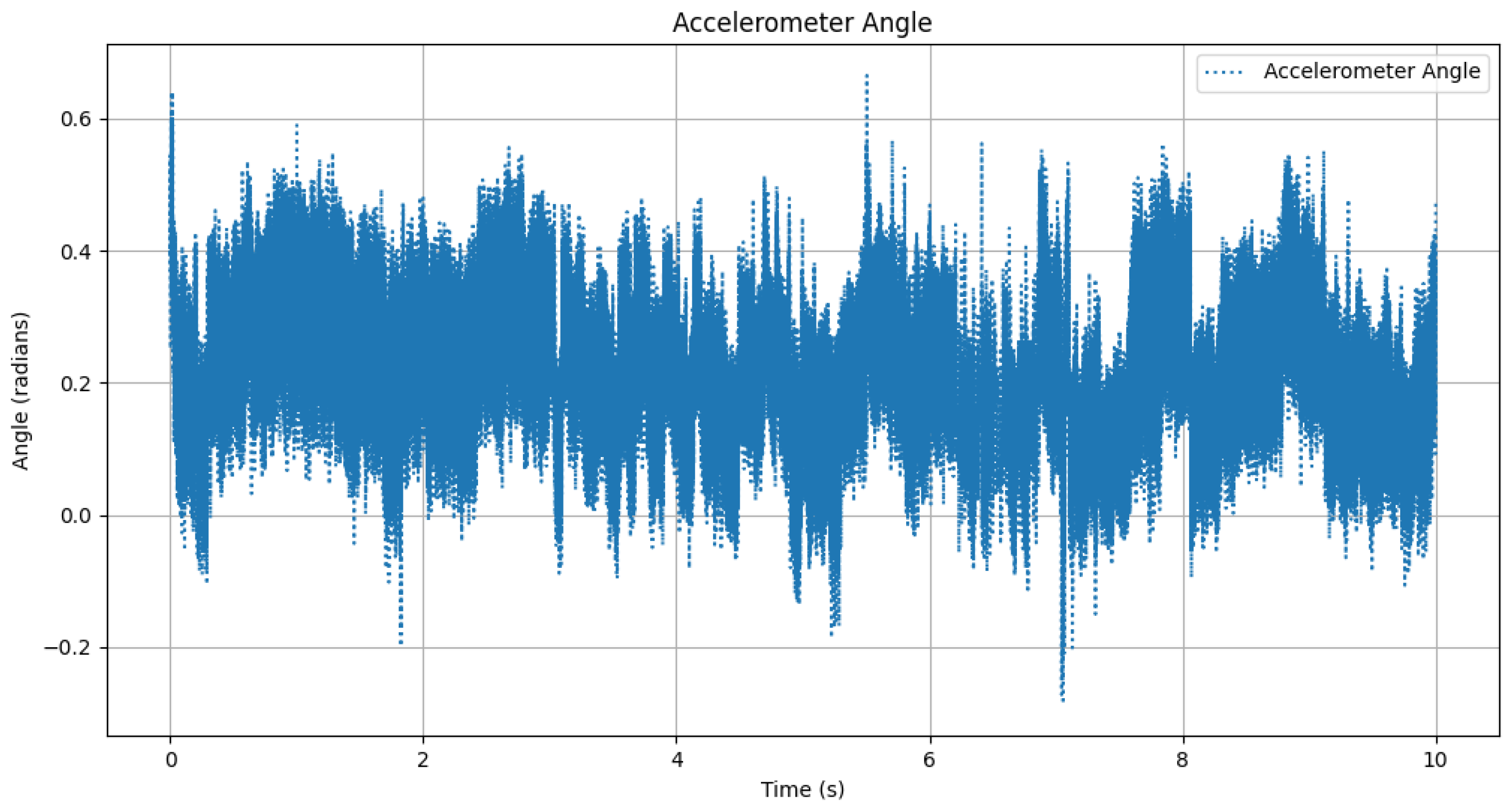
Figure 2 and Figure 3 present the accelerometer and gyroscope data from Dataset1, respectively. Figure 4 and Figure 5 show the corresponding accelerometer and gyroscope data from Dataset2. As indicated by the sensor data from Dataset1 [23], the sampling rate stands at 10 Hz, while it stands at 100 Hz in Dataset2 [24].

Figure 2. Accelerometer data from Dataset1 [23].

Figure 3. Gyroscope data from Dataset1 [23].

Figure 4. Accelerometer data from Dataset2 [24].

Figure 5. Gyroscope data from Dataset2 [24].

This study concentrates solely on X-axis sensor fusion to simplify the conceptual explanation to extend complete sensor fusion across all axes in future work.

5.1. Complementary Filter Result

When applying the complementary filter for sensor fusion, an appropriate value for $\alpha$ must be chosen to control the relative contribution of each sensor. In this research, we have set $\alpha$ to 0.98 for both datasets, signifying that gyroscope sensor data hold much more significance for our specific application. 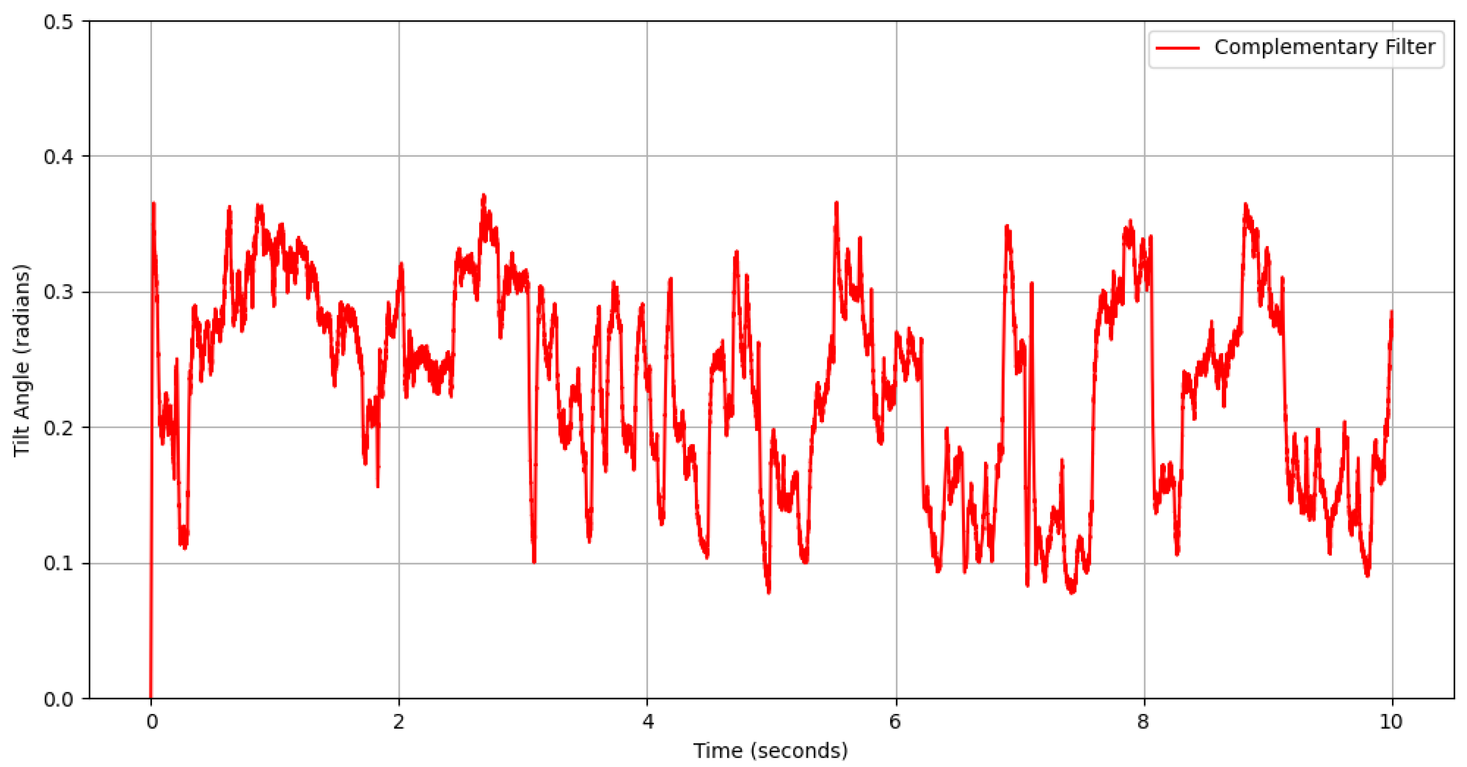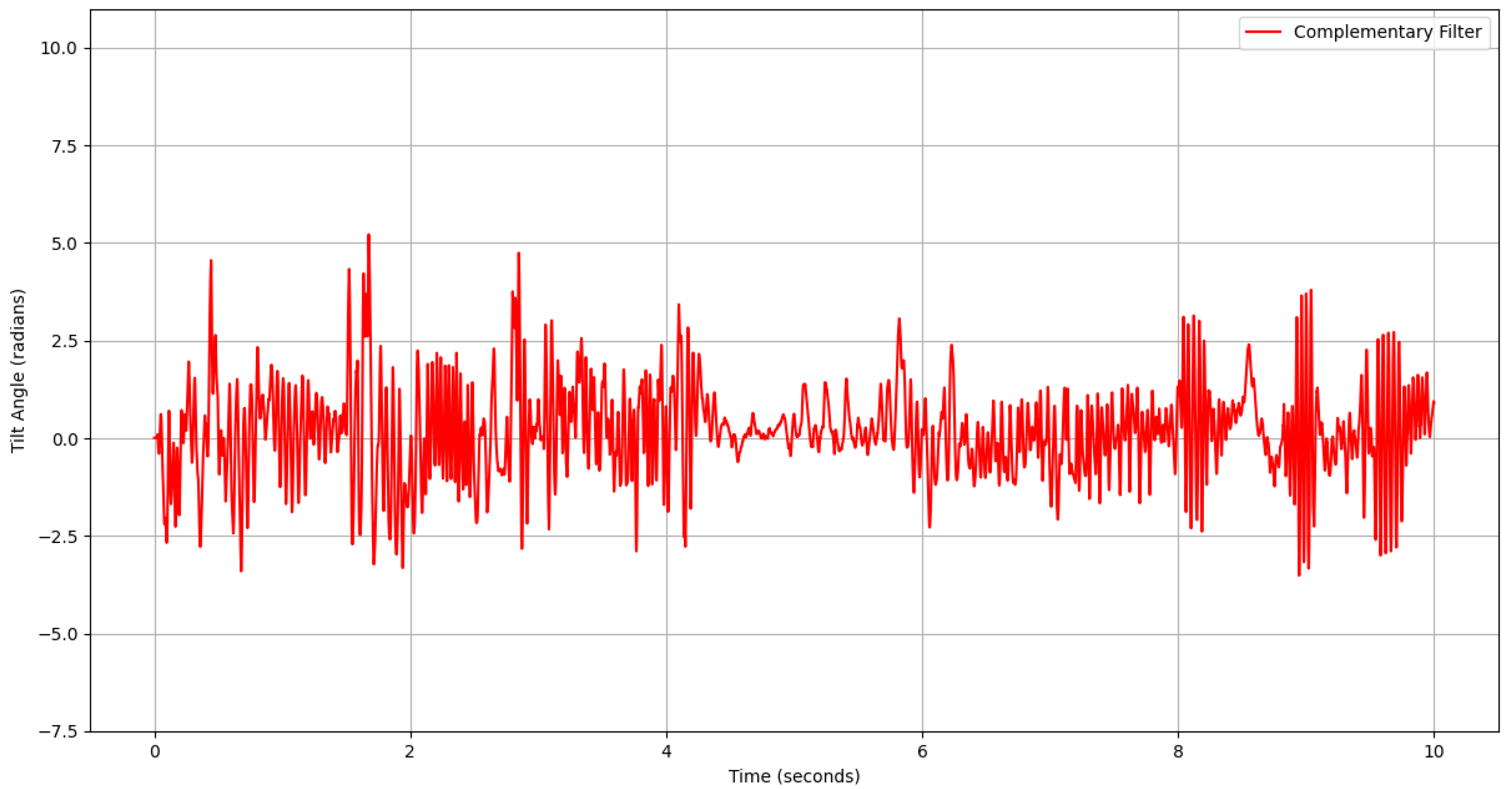Given that the sampling rates are 10 Hz for Dataset1 and 100 Hz for Dataset2, the value of $dt$ is set to 0.1 s for Dataset1 and 0.01 s for Dataset2, corresponding to the inverse of the sampling rates, providing the time interval between the samples. The angles obtained through the complementary filter are illustrated in Figure 6 and Figure 7 corresponding to Dataset1 and Dataset2, respectively.

Figure 6. Complementary filter sensor fusion solution for Dataset1.

Figure 7. Complementary filter sensor fusion solution for Dataset2.

5.2. Kalman Filter Result

The Kalman filter is an essential algorithm for sensor fusion, and its effectiveness hinges on the appropriate selection of its parameters: the process noise covariance (Q), the measurement noise covariance (R), and the estimation error covariance (P). These parameters are pivotal in determining the filter’s precision and stability. In this study, for both datasets, the values of Q, R, and P were carefully set to $0.00001$, $0.5$, and 1, respectively, after a series of calibration tests.

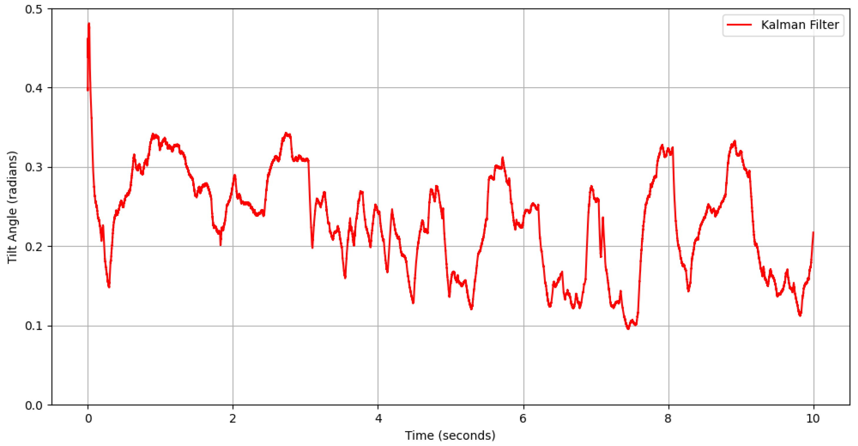
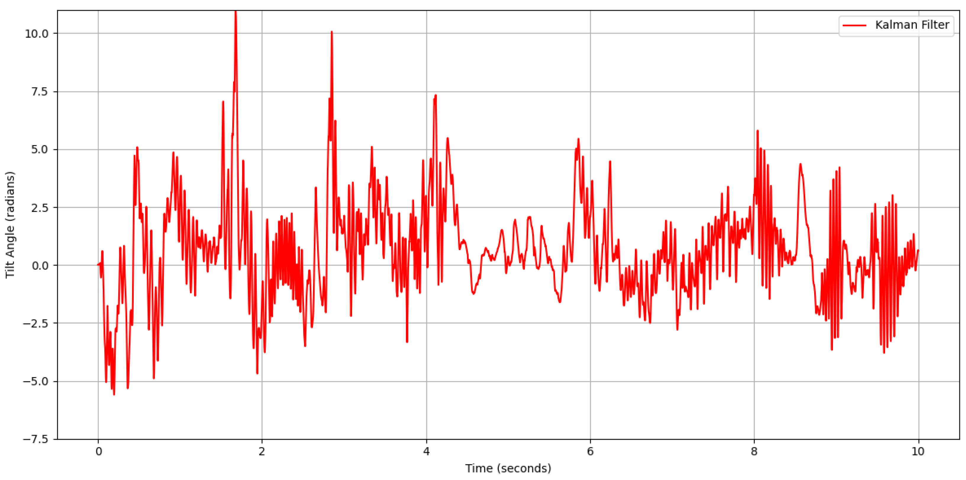
A low Q value reflects high confidence in the model’s accuracy and a moderate R value recognizes sensor noise. The initial P value indicates uncertainty in the initial estimate, which the Kalman filter iteratively improves. The resulting fused angles are depicted in Figure 8 and Figure 9, corresponding to Dataset1 and Dataset2, respectively. These results show a refined, smooth estimate, highlighting the filter’s effectiveness in noise reduction for applications such as robotics and vehicle orientation requiring precision.

Figure 8. Kalman filter sensor fusion solution for Dataset1.

Figure 9. Kalman filter sensor fusion solution for Dataset2.

5.3. Hybrid Approach Result

The main idea behind the hybrid approach lies in the concept of nonlinear smoothing; hence, Schreiber’s filter is applied to the outcome of the complementary filter. This section aims to show the adaptability and effectiveness of nonlinear filtering in sensor fusion. First, filter parameters are chosen, including time delay, dimension, neighborhood size, and downsample factor. The chosen parameters are shown in Table 1.

Table 1. Nonlinear filter parameters.

Time Delay	Dimension	Neighborhood Size	Downsampling Factor
50 ms	8	200	5

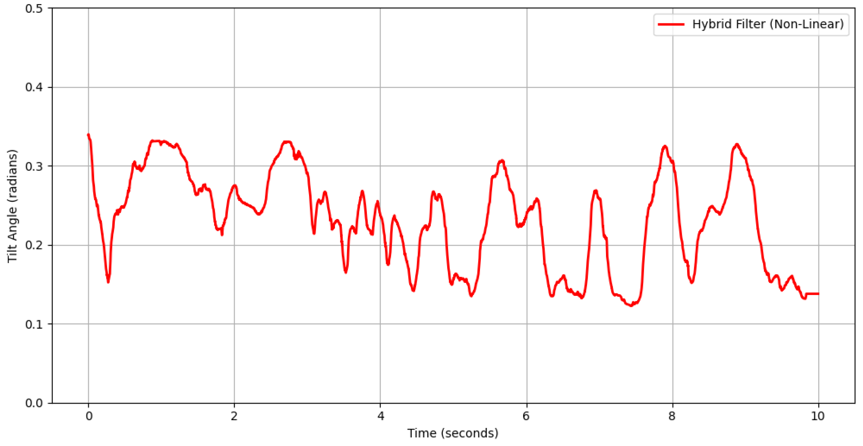
The results of the proposed hybrid sensor fusion method, using the parameter values outlined in Table 1, are presented in Figure 10 and Figure 11, corresponding to Dataset1 and Dataset2, respectively.

Figure 10. Hybrid approach sensor fusion solution for Dataset1.

Figure 11. Hybrid approach sensor fusion solution for Dataset2.

Figure 12 and Figure 13, corresponding to Dataset1 and Dataset2, respectively, illustrate the outcomes of the three sensor fusion techniques to clarify their differences.

Figure 12. Comparison of sensor fusion solutions from three approaches for Dataset1.

Figure 13. Comparison of sensor fusion solutions from three approaches for Dataset2.

For both datasets, the proposed hybrid sensor fusion approach produces smoother outputs than the complementary and Kalman filters, offering enhanced stability, robustness against noise, and improved signal refinement. Its ability to effectively mitigate noise while preserving system responsiveness highlights its advantage in reliable downstream processing.

It is important to note that the nonlinear filtering method was applied to the outputs of the Kalman and complementary filters rather than directly to the sensor fusion process itself. Practical factors led to this choice: real-time phase-space reconstruction and manifold-based projection require substantial computational resources that exceed the processing capabilities of the available embedded platform. To assess the denoising efficacy of nonlinear filtering without sacrificing real-time performance, it was applied as a post-processing step.

Effect of Parameter Selection on Filtering Performance

The effectiveness of the proposed hybrid nonlinear filtering method depends critically on the appropriate selection of several key parameters such as time delay, embedding dimension, neighborhood size, and downsampling factor. Each plays a distinct role in shaping the phase-space reconstruction and the quality of local manifold estimation used in the projection step:

• The distance between delayed locations in the reconstructed vectors is determined by time delay ($\tau$). A compressed attractor results from successive coordinates becoming highly coupled if $\tau$ is too tiny. On the other hand, a high $\tau$ could result in the breakdown of significant dynamic connections. In order to preserve projection stability and uncover the underlying system dynamics, choosing an appropriate delay is vital.
• The number of delayed coordinates needed to reconstruct the phase space is defined by the dimension m. While a dimension that is too high increases computational complexity and noise susceptibility, a value that is too low may fail to unfold the attractor, causing projection errors. A well-balanced decision guarantees adequate system dynamics reconstruction with effective computation.
• The tangent space around each reconstructed point is estimated using the local neighborhood. Although a large neighborhood may smooth out significant nonlinear features, a small neighborhood may be susceptible to noise and capture fine-grained local dynamics. The selected neighborhood must provide consistent covariance estimates while preserving the intrinsic geometry of the attractor.
• Downsampling reduces the number of data points processed during filtering, making the method computationally more tractable. However, excessive downsampling can remove relevant temporal details and distort the reconstructed attractor. A moderate factor ensures efficient computation without sacrificing critical system information.

These parameters must be carefully tuned to balance denoising performance, structural fidelity, and runtime feasibility. Their impact is particularly significant in resource-constrained environments, where both computational cost and filtering quality are critical considerations.

6. Conclusions and Future Work

This study presented a novel hybrid sensor fusion approach that combines conventional sensor fusion methods such as the Kalman and Complementary filters with Schreiber’s nonlinear filter. The method was employed on IMU data, where the gyroscope and accelerometer signals were merged using standard techniques and then enhanced through nonlinear phase-space reconstruction. The findings show that, compared to standalone filtering techniques, the suggested approach offers better noise reduction, increased robustness against outliers, and improved stability.

The hybrid approach preserves important signal aspects while reducing noise by using local manifold projections and delay-coordinate embedding to effectively capture the system’s nonlinear characteristics. According to the results, the Schreiber-based hybrid approach outperforms both the Kalman and Complementary filters in terms of preserving signal integrity and minimizing artifacts, which makes it a viable substitute for applications in unpredictable and dynamic settings.

Future research can enhance the proposed strategy through automatic parameter tuning using algorithms such as PSO or Bayesian optimization to improve filtering performance. A comparative analysis involving UKF, particle filters, and deep learning models could further validate its effectiveness. Moreover, implementing the hybrid filtering method in robotic systems [25], such as those used for perception or motion planning tasks [26], will evaluate its practical feasibility in real-time applications. This approach could yield promising results for autonomous systems, potentially contributing to the future of transportation systems. Future studies will also concentrate on applying nonlinear filtering to enable real-time sensor integration. Because nonlinear filtering is computationally expensive, it is used as a post-processing step in the current implementation. Future research will focus on finding quicker and more affordable solutions that enable integration into real-time systems, especially in situations with constrained hardware resources.

Furthermore, it offers significant promise for improving future transportation systems with the suggested hybrid sensor fusion technique. Specifically, typical sensor fusion algorithms may not be able to guarantee safety and accuracy in highly dynamic and nonlinear settings which will arise in the context of autonomous cars, drones, and intelligent traffic networks [27,28]. The use of the nonlinear filtering approach in autonomous driving frameworks will be examined in future research, with an emphasis on problems like multi-agent vehicle cooperation, chaotic traffic situations, and unpredictable pedestrian behavior. The robustness of the method under actual transportation situations will be validated through real-world trials using mobile robots and simulated autonomous cars.