Abstract
Magnetic Resonance Relaxometry is a powerful technique that reveals a sample’s molecular dynamics thanks to the dependence of the T1 relaxation time on field strength. With applications in protein research, food systems, material development, and environmental science, relaxometry measurements are typically undertaken using a technique known as fast field cycling, where T1 is measured at a range of detection fields. However, the sample experiences relaxation in a variable field without the challenges associated with retuning a probe to each of the necessary frequencies of interest. This technique is limited by a maximum relaxation time, since the measurement and relaxation fields are typically applied using a fluid-cooled electromagnet, which will ultimately overheat for very long experimental times. In this work, we propose an alternative approach to permit measurements of samples with inherently long T1 values. We utilise a broadband spectrometer alongside a solenoid transmit-receive coil and custom tuning and matching boards, whilst two sets of magnets are moved around the coil, to achieve a range of different fields. By collecting a reduced number of points and utilising this method, we show it is still possible to make useful measurements on samples at a range of frequencies, which has great potential in quality assurance applications. We find a similar trend for food samples of corn oil, while manganese chloride, a common contrast agent, has more than a 100% difference when compared to traditional fast field cycling measurements.
1. Introduction
Spin-lattice, or longitudinal, relaxation is the process of a nuclear system’s net magnetisation (M) returning to its initial maximum value (M0) following excitation by application of radio frequency energy [1]. Energy is transferred to neighbouring molecules, the magnitude of which is given by Equation (1) [2]:
where Mz is the net magnetisation along the z-axis, M0 is the initial magnetisation, τ is the measurement time, and T1 is a sample property characterisation this exchange of energy. Measuring T1 reveals interesting sample properties, such as molecular viscosity and protein morphology. To do so, several data points must be acquired, to which an exponential with time constant T1 is fitted. Such an experiment is the inversion recovery experiment, where the magnetisation is initially inverted by applying a radiofrequency (RF) pulse of 180° before allowing the system to relax for a time (τ). Following this delay, a 90° RF pulse is applied, and the resulting free induction decay (FID) is Fourier-transformed to provide a spectrum. The intensity of the spectral peaks is then plotted against the varying τ values [3]. The value of T1 is defined as the time taken for Mz to return to ~63% of its original value. It typically takes a spin system 5xT1 to recover 99% of its original equilibrium magnetisation.
T1 is also dependent on the magnetic field strength, with interesting features encoded in the relationship between T1 and field strength. It is, for example, possible to measure the coupling of protons to nitrogen atoms by measuring T1 at the field strengths where the nitrogen quadrupolar coupling coincides with the proton frequency [4]. Measurement of the variation of T1 with field strength is commonly achieved using fast field cycling (FFC) experiments. An FFC relaxometry experiment consists of a repeated T1 measurement pulse sequence, such as an inversion recovery sequence which can be seen in Figure 1.
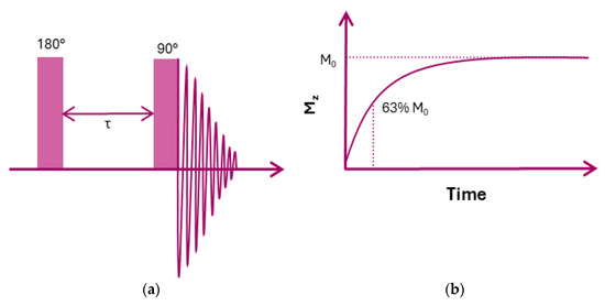
Figure 1.
(a) Pulse sequence diagram for an inversion recovery experiment and (b) model of the longitudinal relaxation process.
The excitation occurs at the same field strength, and the FID is detected at the same detection field for each repetition; however, a relaxation field (and therefore the Larmor frequency) is varied. A graph of the relaxation rate (1/T1) against the range of Larmor frequencies can then be produced.
Typical field cycling experiments will consist of either a pre-polarised (PP) or non-polarised (NP) sequence (Figure 2). During a PP sequence, the sample will first build up an equilibrium magnetisation in a polarisation field for a period dp, before switching to a lower relaxation field where the spin system relaxes to a new equilibrium magnetisation value. It will then switch to a detection field where the 90° RF pulse is applied, and the resulting FID detected. The time needed to switch between these fields is defined as the switching time sw. During a NP sequence, there is no polarisation field, and the equilibrium magnetisation is instead built up in the relaxation field. PP sequences allow for the exploration of much lower fields, whilst NP sequences are used to bridge the gap between these fields and the fields at which more conventional techniques can be used [5].
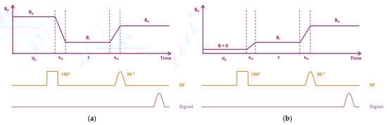
Figure 2.
(a) PP sequence and (b) NP sequence.
One of the main drawbacks of FFC systems is that they require robust cooling systems and are expensive to purchase. Furthermore, to prevent overheating of the magnetic field coils, they are restricted to the exploration of samples with relatively short T1 limiting their applicability to low concentrations of aqueous samples. A block diagram of a typical FFC system can be seen in Figure 3 [3]. It is the goal within this work to produce a lower cost system that utilises permanent magnets that can be moved relative to the sample to obtain varying field strengths and use this setup to show comparable results with an existing FFC system across a select range of Larmor frequencies.
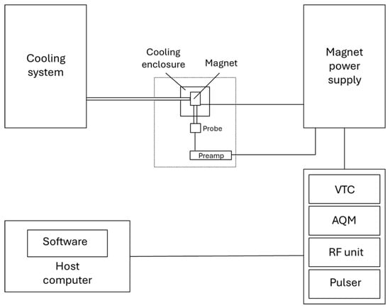
Figure 3.
FFC instrument with variable temperature controller (VTC) and acquisition module (AQM). The dashed box represents the part of the commercial FFC system which we are seeking to replicate using a permanent magnet-based system.
2. Materials and Methods
Two pairs of 50 × 50 × 10 mm N45 Neodymium magnets (Magnosphere, Troisdorf, Germany) were assembled in acrylic holders and mounted onto lengths of M10 threaded rod. These were secured in place using a set of 16 nuts, one either side of the holders at both ends. Steel yokes measuring 100 × 40 × 10 mm were added to the outer faces of the magnets, with an additional 250 × 40 × 10 mm length underneath to produce a more stable magnetic field in the central region for measurements by providing a return path for the stray magnetic field. This setup can be seen below in Figure 4.

Figure 4.
Photograph of variable field sensor showing variable position magnet housings and suspended RF coil and sample.
The spacing between the two sets of magnets is currently manually adjusted by moving the nuts. This will be automatable by using reverse thread nuts on one acrylic holder and a stepper motor geared to the threaded rods. The resulting field was then measured to determine the tuning frequency for the coil using a gauss meter (HM08 Hirst Magnetics, Falmouth, UK). With this setup, it is possible to achieve a maximum field strength of up to 400 mT.
A single-layer 13-turn copper solenoid coil was tuned to each individual measurement field using a custom tuning and matching board, from a range of 300 mT (12.7 MHz) down to 200 mT (8.5 MHz). Shielding was also placed around both the coil and the tuning and matching board to improve the signal-to-noise ratio (SNR) in electrically noisy environments. The sample was positioned within the field using a retort stand and clamp.
Using a benchtop NMR console (Kea2, Magritek, Wellington, New Zealand), a series of T1 inversion recovery experiments were run for two samples. Each scan consisted of 64 averages across a τ range of 1 ms–1000 ms for a sample of corn oil, and a range of 1 ms–150 ms for a sample of MnCl2.
Identical samples were also analysed using a FFC NMR relaxometer (SPINMASTER, Stelar, Mede, Italy) across a frequency range of 15 MHz to 5 MHz using a NP sequence with 8 averages. The samples were kept at room temperature (293 K) for the duration of the scans.
3. Results and Discussion
Figure 5 shows a comparison between the results obtained using the FFC relaxometer and the variable field sensor for both corn oil and MnCl2. The relaxation rate for both samples obtained using this system follows the expected trend with increasing Larmor frequency; however, as can be seen, there is a significant difference between these values and those obtained using the FFC relaxometer, which is more pronounced for the manganese chloride samples.
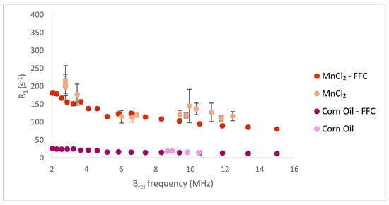
Figure 5.
Plot of resulting relaxation rates against frequency for samples of MnCl2 and corn oil using both the new magnet system and the FFC relaxometer.
Errors in the results obtained by the new system for both samples are also notably larger than for the FFC relaxometer. There are several potential contributing factors to this, the most prominent likely being that the field within the centre of the magnets is not as stable as it would ideally be for these measurements, and therefore it is likely that the sample is sitting over a range of different field strengths. This could be rectified in the future by improving the design of the yokes for a more stable central field or the inclusion of shaped pole pieces. A more accurate method for positioning the sample within the field as well as improved shielding for both the sample and the tuning and matching board would also help with reducing the noise and the errors in the measurements.
These preliminary results require further investigation to using a greater range of concentrations to better understand the source of the discrepancy.
4. Conclusions
We have presented preliminary results demonstrating the ability of an automatable permanent magnet sensor to create a T1 frequency dispersion plot akin to that of a fast field cycling system. There is, however, a significant discrepancy between the results of a traditional fast field cycler and our new sensor, which requires further investigation. This will include the measurement of different paramagnetic agents at different concentrations to determine if the offset is consistent or variable.
Further development is needed to improve this system, including enhancing the stability of the field in the centre of the magnets with better positioned and designed yokes. Improvements to the SNR could also be made by increasing the number of averages per scan and further tweaks to the shielding around the coil and tuning and matching board. It would also be beneficial to investigate a wider range of frequencies to better test and understand the limits of the system. Once this optimisation is concluded, the system can be automated to provide automatic measurements of T1 dispersion.
Author Contributions
Conceptualization, all authors.; methodology, K.W. and R.H.M.; validation, K.W.; formal analysis, K.W.; investigation, K.W.; resources and initial hardware development, N.R.G.; writing—original draft preparation, K.W.; writing—review and editing, all authors.; supervision, R.H.M. and M.I.N.; funding acquisition, R.H.M. and M.I.N. All authors have read and agreed to the published version of the manuscript.
Funding
This manuscript is part of a project that has received funding from the European Union’s Horizon 2020 research and innovation program under the Marie Skłodowska-Curie grant agreement No 101008228. The authors wish to express their thanks to EUH2020 for this funding and to Nottingham Trent University for match funding K.W.’s PhD programme.
Institutional Review Board Statement
Not applicable.
Informed Consent Statement
Not applicable.
Data Availability Statement
The data which has been used in the preparation of this manuscript has been made available in Zenodo repository 10.5281/zenodo.17815833.
Conflicts of Interest
The authors declare no conflict of interest.
References
- Dale, B.M.; Brown, M.A.; Semelka, R.C. MRI Basic Principles and Applications, 5th ed.; John Wiley and Sons, Inc.: Hoboken, NJ, USA, 2015. [Google Scholar]
- Fukushima, E.; Roeder, S.B.W. Experimental Pulse NMR: A Nuts and Bolts Approach; CRC Press: Boca Raton, FL, USA, 1981. [Google Scholar]
- Keeler, J.J. Understanding NMR Spectroscopy, 2nd ed.; John Wiley and Sons, Inc.: Hoboken, NJ, USA, 2010. [Google Scholar]
- Broche, L.; Pine, K.; Ismail, S.; Davies, G.; Lurie, D. Nitrogen-proton cross-relaxation in Fast Field-cycling MRI. In Proceedings of the 19th JSPS Core-to-Core Seminar, Fukuoka, Japan, 4 February 2012. [Google Scholar]
- Anoardo, E.; Galli, G.; Ferrante, G. Fast-Field-Cycling NMR: Applications and Instrumentations. Appl. Magn. Reson. 2001, 20, 356–404. [Google Scholar] [CrossRef]


Disclaimer/Publisher’s Note: The statements, opinions and data contained in all publications are solely those of the individual author(s) and contributor(s) and not of MDPI and/or the editor(s). MDPI and/or the editor(s) disclaim responsibility for any injury to people or property resulting from any ideas, methods, instructions or products referred to in the content. |
© 2025 by the authors. Licensee MDPI, Basel, Switzerland. This article is an open access article distributed under the terms and conditions of the Creative Commons Attribution (CC BY) license (https://creativecommons.org/licenses/by/4.0/).