Abstract
Reinforcement learning, particularly Q-learning, has demonstrated significant potential in autonomous navigation applications. However, the environments of the real world introduce sensor noise, which can impact learning efficiency and decision-making. This study examines the influence of sensor noise on Q-learning performance by simulating an agent navigating an environment with noise. We compare two learning strategies: one with fixed hyperparameters and another with dynamically adjusted hyperparameters. Our results show that high sensor noise degrades learning performance, increasing convergence time and sub-optimal decision-making. However, adapting hyperparameters over time improves resilience to noise by optimizing the balance between exploration and exploitation. These findings highlight the importance of robust learning strategies for autonomous systems under uncertain conditions.
1. Introduction
Reinforcement learning (RL) enables autonomous agents to navigate in complex environments. Among the various reinforcement learning techniques, Q-learning has taken over for its effectiveness in decision-making and trajectory optimization. However, in real-world cases, to collect environmental data, autonomous systems rely on perception sensors that are often affected by noise, which is due to environmental factors, hardware limitations, or signal interference, introducing inaccuracies that impact an agent’s learning process and overall navigation performance. To develop more robust and adaptive learning strategies, it is necessary to first understand the influence of sensor noise on Q-learning. While traditional Q-learning approaches assume relatively stable and accurate state representations, real-world conditions require learning models that can withstand uncertainty.
Mobile robotics includes aspects such as perception, decision-making, and navigation [1]. This cycle is crucial for autonomous systems, which all rely on well-defined sensor data. Perception is dedicated to collecting and interpreting environmental information using sensors such as Light Detection and Ranging (LiDAR), cameras, radar, and ultrasonic sensors [2]. However, when perception is compromised by noise caused by environmental factors, hardware limitations, and signal interference, the system can generate inaccurate state representations, leading to decision-making errors and sub-optimal navigation strategies [2].
In reinforcement learning navigation, decision-making depends on the agent’s ability to evaluate states and select optimal actions based on learned policies. Noisy sensor data can cause the agent to misperceive the environment, which may lead it to make wrong decisions or fail to recognize obstacles and optimal paths [3,4]. To ensure robust performance in real-world conditions, and to avoid reduced efficiency, impaired navigation performance, and increased time to reach a goal, it is essential to develop learning strategies that account for sensor noise. Adaptive techniques, such as dynamic hyperparameter tuning, sensor fusion, and noise filtering, can help reduce the negative effects of noise, thereby improving perception accuracy and decision-making efficiency [3,4]. These strategies enable more reliable navigation in complex and unpredictable environments by improving the agent’s ability to process uncertain data.
Recent works related to sensor noise impact, such as the study of Lee, Theotokatos, and Boulougouris, explore the impact of sensor noise on decision-making for reactive collision avoidance in autonomous ships using a deep reinforcement learning agent trained with varying noise levels, highlighting the importance of incorporating noise variance observations to enhance the robustness and safety of decision-making in uncertain environments [5]. Van Brummelen, O’Brien, Gruyer, and Najjaran’s article offers a comprehensive review of state-of-the-art autonomous vehicle (AV) perception systems, examining the advantages, disadvantages, and ideal applications of various sensors, as well as current localization and mapping methods, identifying future research areas to enhance AV robustness, safety, and efficiency [6]. The paper of Tiwari, Srinivaas, and Velamati explores a reinforcement learning-based approach that integrates GPS, magnetometer, and ultrasonic sensors to enhance autonomous vehicle navigation, improving accuracy, adaptability, and efficiency in dynamic environments [7]. Vladov, Vysotska, Sokurenko, Muzychuk, Nazarkevych, and Lytvyn present an advanced neural network system for intelligent monitoring and anomaly detection in helicopter turboshaft engines, integrating SARIMAX and LSTM-based models to achieve high prediction accuracy while addressing sensor malfunctions and external noise factors [8].
Our study compares two learning strategies: one with fixed hyperparameters and the other with dynamically adjusted hyperparameters to explore the effects of sensor noise on Q-learning performance by simulating an agent navigating in a grid-based environment. This study analyzes convergence time, decision-making efficiency, and overall learning performance. Our results highlight the importance of adaptive learning techniques that optimize the balance between exploration and exploitation, thus improving the robustness of autonomous systems in uncertain environments.
2. Overview of Q-Learning and Perception Sensors
2.1. Materials and Methods
To assess how sensor noise affects Q-learning performance, we conducted a series of MATLAB R2021a simulations in a grid-based environment designed to mimic real-world autonomous navigation. The goal was to see how an agent, guided by a Q-learning algorithm, adapts to noisy sensor data while trying to reach a target location.
Two distinct learning strategies were compared, as shown in Figure 1: one where the hyperparameters remained fixed throughout the experiment, and another where the hyperparameters were dynamically adjusted based on the agent’s performance. The key hyperparameters, including the learning rate, discount factor, and exploration rate, were varied in the dynamic strategy to optimize the agent’s learning process over time. The experiments involved training the agent in environments with different levels of noise, ranging from low to high, to assess the impact on convergence time, decision-making accuracy, and the agent’s ability to balance exploration and exploitation.
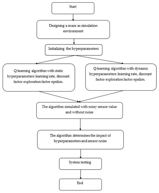
Figure 1.
Block diagram of the methodology and design.
2.2. Sensors
The essential part for robots and autonomous vehicles is perception sensors, which allow them to collect and interpret data about their environment. These sensors provide crucial information for navigation, object detection, and decision-making. However, each type of sensor is susceptible to different types of noise, which can affect the accuracy and reliability of the collected data [9]. Noise can come from various factors, such as environmental conditions, sensor limitations, or signal interference. To improve the performance of sensors through filtering, sensor fusion, or calibration techniques [10], it is necessary to understand these noise characteristics. Table 1 presents an overview of the different perception sensors, their functions, advantages, limitations, and the types of noise that affect them.

Table 1.
Comparison of perception sensors [10].
2.3. Reinforcement Learning
RL is a type of machine learning based on the concepts of agent, environment, and rewards, where an agent learns to make decisions by interacting with an environment, with the goal of maximizing a cumulative reward over time by taking actions that lead to better outcomes [11], and also by learning the optimal policy that maximizes the cumulative reward, often formalized by [11].
where γ is the discount factor that controls how much future rewards are valued compared to immediate ones, and T is the time horizon. Figure 2 shows the reinforcement learning principle.
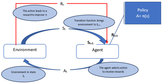
Figure 2.
Reinforcement learning principle [12].
2.3.1. Q-Learning
Q-learning is a model-free reinforcement learning algorithm used to find the optimal action selection policy. It is based on learning the Q-values, which represent the expected future reward of taking a particular action in a given state [13].
The Q-function, denoted as Q(s, a), is the expected discounted future reward that can be obtained by taking action, a, in state, s, and then following the optimal policy.
In Q-learning, the agent learns the Q-values iteratively using the Bellman equation, as shown in Equation (2) [13]:
New Q(s, a) ← Q(s, a) + α [r + γ maxa′,Q′(s′, a′) − Q(s, a)]
2.3.2. Hyperparameters
Hyperparameters are essential in the formation of how a Q-learning agent learns, explores his environment, and finally finds the best strategy. The choice of good values for these parameters can make the difference between an agent who learns effectively and an agent who is stuck in under-optimal behavior. The learning rate (α) controls the speed with which the agent updates his knowledge, balancing speed, and stability. The update factor (γ) determines whether the agent prioritizes short-term or long-term rewards [14]. The ϵ greedy strategy manages exploration in relation to exploitation, with adaptive techniques improving learning over time. The initialization of value Q affects early exploration, while update methods influence the stability of learning. The dynamic adjustments to these parameters improve resilience in noisy or uncertain environments, guaranteeing more reliable and more efficient autonomous decision-making [14].
One of the biggest challenges in Q-learning is to find the right balance between exploration and exploitation [15], where hyperparameters have a direct impact on this balance. If the learning rate is too high, the agent may find it difficult to stabilize; if it is too low, learning can be too slow. Likewise, the exploration rate must be carefully adjusted as too much randomness can prevent convergence, while too little can cause premature optimization [15].
Static hyperparameter values may not always be effective since real world environments are often dynamic and unpredictable. The techniques explored by researchers to optimize these parameters help to improve the efficiency of learning and robustness, particularly in complex environments with a sensor noise or changing conditions. Understanding the role of hyperparameters and how they affect Q-learning is fundamental for the design of intelligent and effective strengthening learning systems. By carefully adjusting these parameters, we can improve the ability of an agent to learn, adapt, and make better decisions in uncertain environments.
3. Results
No sensor is perfect in real-world applications. The environmental conditions or even the internal components of the sensor can introduce errors or “noise” in the measured values of the sensor. By adding Gaussian noise to the real distance, you model the fact that the readings of the sensor will fluctuate around the true value in a random manner.
In the context of Q-learning, the noisy distance has an impact on how the agent perceives his environment. When the agent receives noisy comments from his sensors (in this case, noisy distance measures), he must learn to adapt his decision to compensate for this uncertainty. The agent can take a little more time to achieve the objective or choose different actions depending on the randomness introduced by the noise. By translating this type of noise in our simulations, we are testing the robustness of the Q control algorithm and the impact of the sensors on its learning.
The simulations made by measuring the distance to the objective were simulated with LiDAR sensors and ultrasonic sensors to represent the current perception sensors used in autonomous robots. The LiDAR sensor model captures the distance with high precision but is affected by environmental factors such as fog or reflections. The ultrasonic sensor model, which is simpler and often used in robotics, introduces noise based on acoustic interference and surface properties. The noise in distance measurements has been linked to the model using the Gaussian noise, N (0, σ), where the standard deviation (σ) of the noise reflects the inaccuracies of typical sensors, representing scenarios of the real world where environmental factors introduce the variability of the readings of the sensor.
noisy_distance = true_distance + N(0, σ)
- True distance: It is the real and precise distance measured by the sensor under ideal conditions, without any interference of the noise or environmental factors, between the agent and the objective or the obstacle.
- Noise (N (0, σ)): It represents Gaussian noise (also known as normal distribution noise) with an average of 0 and a standard σ σ. Gaussian distribution is often used to model noise because of the many phenomena in the real world. The average of 0 means that noise does not have a coherent bias in a direction, and that noise is also likely to be positive by adding to the distance, or negative by removing distance.
- σ: It is the standard noise deviation, which controls the variability of space or noise. A higher value of σ means greater random variability of noisy measurements, while a smaller σ means less noise.
- Noisy distance: This is the measured final distance, including real distance and random noise. The noisy distance represents the perception of the sensor after having taken into account the conditions of the real world such as the imperfections of the sensors, the external factors, or the random disturbances.
In this section, we compare two approaches: Q-learning with static hyperparameters and Q-learning with dynamic hyperparameters. For both of them, we simulate the algorithm by including noise of sensors to evaluate the impact and relationship between sensors that represent the external environment and hyperparameters for the learning of the agent. Our environment is represented in Figure 3, where the starting point is the agent (robot) marked in green, the goal to reach is marked in red, and the obstacles to avoid are the back walls. And Table 2 represents the quantitative complexity of environment.
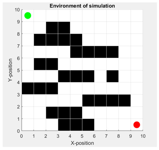
Figure 3.
Simulation environment where the starting point is the agent (robot) marked in green, the goal to reach is marked in red, and the obstacles to avoid are the back walls.
Table 2.
Quantitative complexity of environment.
Figure 4a shows the results of the first case where the agent learns through Q-learning with constant hyperparameters: alpha = 0.1, gamma = 0.9, and epsilon = 0.1. Sensor noise is introduced to affect the agent’s ability to estimate distances to the goal. The agent’s task is to navigate the maze with and without noise.
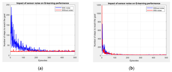
Figure 4.
Q-learning results with constant hyperparameters (a) and Q-learning results with dynamic hyperparameters (b).
- Without Noise: In simulations, the agent finds the objective in fewer steps as the algorithm of Q-learning converges.
- With Noise: The performance of the agent is disturbed by the sound of the sensor. It takes more measures to achieve the objective because the distance to the objective is uncertain due to noise. This is reflected in the greater number of steps per episode with noise.
- Convergence Speed: Without noise, the agent converges more quickly to optimal policy compared to the agent with rough sensor values.
- Steps per Episode: In the noisy case, the agent takes more measures to achieve the objective due to uncertainty in the calculation of the reward.
- Exploration vs. Exploitation: In both cases, the Epsilon-Greedy policy will ensure a certain level of exploration. However, the agent with noise explores more because his reward function is less reliable.
Figure 4b shows results where the agent learns through Q-learning but this time with dynamic learning parameters, namely alpha, gamma, and epsilon, which change over time. The initial values for alpha, gamma, and epsilon are higher and decay over episodes, as shown in Figure 5:
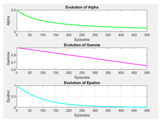
Figure 5.
Dynamic changes in the hyperparameters.
- Alpha: Decreases with each episode, allowing the agent to stabilize its learning as it gains more experience.
- Gamma: Decreases slightly, which may reduce the importance of future rewards over time.
- Epsilon: Decreases exponentially, promoting more exploitation of learned actions as the agent converges to an optimal policy.
The idea behind dynamic changes is to help the agent refine his strategy over time. The agent begins with more exploration and moves later to exploitation as learning stabilizes. Basically, without noise, the agent learns with fewer steps because the disintegration of exploration allows a more refined policy. The dynamic decrease in alpha and epsilon helps the agent to converge faster. With noise in the noisy environment, it means that the agent takes more time to reach the goal in relation to the noise-free scenario. The dynamic adjustments always allow the agent to improve over time, but the readings of noisy sensors will probably lead to more exploration in the first episodes.
- Convergence Speed: Dynamic hyperparameters accelerate convergence in noisy and noise-free cases. The decomposition of alpha and epsilon ensures that the agent turns to the exploitation of knowledge learned more quickly, improving efficiency.
- Impact of Noise: Despite the dynamic hyperparameters, noise always affects the agent’s performance, resulting in a higher number of steps by episode when noise is present.
- Hyperparameter Evolution: The graphs showing the evolution of alpha, gamma, and epsilon through the episodes will show how these parameters will decrease over time, allowing better exploitation and stabilization.
4. Discussion
With dynamic hyperparameters, Figure 5 demonstrates more advanced Q-learning behavior. This dynamic adjustment enables faster convergence and more efficient learning compared to a constant hyperparameter setup. However, the impact of sensor noise remains significant, showing that dynamic learning can only partially mitigate the challenges posed by noisy sensors.
In both cases, the sensor noise hinders the agent’s ability to quickly converge towards the goal. The noise increases the number of steps necessary to achieve the objective, demonstrating that the sound of the sensor introduces a significant uncertainty which must be managed in the applications of the world of Q-learning.
This study investigates the impact of sensor noise by introducing Gaussian noise with a standard deviation of σ = 0.2 into the agent’s distance calculations, whereby a value of 0.2 introduces noticeable but not extreme randomness in sensor readings. Lower values with σ < 0.1 has a minimal impact on learning; the agent performs almost as if in a noise-free environment. Higher values of σ > 0.5 introduce too much randomness, making it difficult for the agent to learn an optimal policy. Table 3 resume the effect of σ value on agent’s learning.
Table 3.
Effect of σ value on agent’s learning.
The second case introduces a more adaptive learning strategy with dynamic hyperparameters. By breaking down the alpha, gamma, and epsilon, this configuration allows the agent to focus more on the exploitation of his knowledge as episodes are progressing, potentially leading to better performance in long-term simulations. Although dynamic adjustments improve performance, the sensor noise presence always leads to slower convergence in noisy scenarios compared to noise-free environments.
For learning efficiency, dynamic adaptation of hyperparameters, particularly epsilon, helps the agent to switch from exploration to exploitation, which can lead to faster learning in ideal conditions (noiseless). However, with noise, the agent will still experience more exploratory steps, and the number of steps per episode will likely remain higher in comparison to the noise-free scenario. This case is closer to how real-world systems might adjust their learning parameters over time, which is critical for applications where the environment or sensor data can change. However, as shown by the two configurations, noise remains a critical challenge, requiring other methods such as the fusion of sensors or noise filtering to improve the performance of agents in realistic conditions.
Future studies could focus on manipulation of noise with more advanced techniques to manage noise; as an example, Kalman filtering and the merger of sensors could be integrated to improve the agent’s ability to manage noisy entries and make more precise decisions.
Another hyperparameter adjustment with a fine adjustment to the rate of decomposition of hyperparameters, in particular Epsilon and Alpha, could make new improvements, especially in noisy environments.
Author Contributions
Conceptualization, M.E.W. and M.A.Y.; methodology, M.E.W. and M.A.Y.; software, M.E.W.; validation, M.E.W., M.A.Y., R.D., M.B. and Y.E.K.; formal analysis, M.E.W.; investigation, M.E.W.; resources, M.E.W. and M.A.Y.; data curation, M.E.W.; writing—original draft preparation, M.E.W.; writing—review and editing, M.E.W.; visualization, M.E.W.; supervision, M.A.Y. and R.D.; project administration, M.E.W. and M.A.Y.; funding acquisition, M.E.W. All authors have read and agreed to the published version of the manuscript.
Funding
This research received no external funding.
Institutional Review Board Statement
Not applicable.
Informed Consent Statement
Not applicable.
Data Availability Statement
Data is contained within the article.
Conflicts of Interest
The authors declare no conflicts of interest.
Abbreviations
The following abbreviations are used in this manuscript:
| RL | Reinforcement Learning |
| AV | Autonomous Vehicle |
| LiDAR | Light Detection and Ranging |
References
- Rubio, F.; Valero, F.; Llopis-Albert, C. A review of mobile robots: Concepts, methods, theoretical framework, and applications. Int. J. Adv. Robot. Syst. 2019, 16, 1729881419839596. [Google Scholar] [CrossRef]
- Zhu, W.; Qiu, G. Path Planning of Intelligent Mobile Robots with an Improved RRT Algorithm. Appl. Sci. 2025, 15, 3370. [Google Scholar] [CrossRef]
- Kober, J.; Bagnell, J.A.; Peters, J. Reinforcement learning in robotics: A survey. Int. J. Robot. Res. 2013, 32, 1238–1274. [Google Scholar] [CrossRef]
- Bakir, M.; Youssefi, M.; Dakir, R.; El Wafi, M. Enhancing the PRM Algorithm: An Innovative Method to Overcome Obstacles in Self-Driving Car Path Planning. Int. Rev. Autom. Control (IREACO) 2024, 17, 132–140. [Google Scholar] [CrossRef]
- Lee, P.; Theotokatos, G.; Boulougouris, E. Robust Decision-Making for the Reactive Collision Avoidance of Autonomous Ships against Various Perception Sensor Noise Levels. J. Mar. Sci. Eng. 2024, 12, 557. [Google Scholar] [CrossRef]
- Van Brummelen, J.; O’Brien, M.; Gruyer, D.; Najjaran, H. Autonomous vehicle perception: The technology of today and tomorrow. Transp. Res. Part Emerg. Technol. 2018, 89, 384–406. [Google Scholar] [CrossRef]
- Tiwari, R.; Srinivaas, A.; Velamati, R.K. Adaptive Navigation in Collaborative Robots: A Reinforcement Learning and Sensor Fusion Approach. Appl. Syst. Innov. 2025, 8, 9. [Google Scholar] [CrossRef]
- Vladov, S.; Vysotska, V.; Sokurenko, V.; Muzychuk, O.; Nazarkevych, M.; Lytvyn, V. Neural Network System for Predicting Anomalous Data in Applied Sensor Systems. Appl. Syst. Innov. 2024, 7, 88. [Google Scholar] [CrossRef]
- Abdelhafid, E.; Abdelkader, Y.; Ahmed, M.; Rachid, D.; Abdelilah, E. Visual and light detection and ranging-based simultaneous localization and mapping for self-driving cars. Int. J. Electr. Comput. Eng. (IJECE) 2022, 12, 6284–6292. [Google Scholar] [CrossRef]
- Liu, H.; Li, Y.; Qian, T.; Tang, Y. Recent Progress in Ocean Intelligent Perception and Image Processing and the Impacts of Nonlinear Noise. Mathematics 2025, 13, 1043. [Google Scholar] [CrossRef]
- Terven, J. Deep Reinforcement Learning: A Chronological Overview and Methods. AI 2025, 6, 46. [Google Scholar] [CrossRef]
- El Wafi, M.; Youssefi, M.A.; Dakir, R.; Bakir, M. Intelligent Robot in Unknown Environments: Walk Path Using Q-Learning and Deep Q-Learning. Automation 2025, 6, 12. [Google Scholar] [CrossRef]
- Zourari, A.; Youssefi, M.; Ben Youssef, Y.; Dakir, R. Reinforcement Q-Learning for Path Planning of Unmanned Aerial Vehicles (UAVs) in Unknown Environments. Int. Rev. Autom. Control (IREACO) 2023, 16, 253–259. [Google Scholar] [CrossRef]
- Cho, H.; Kim, H. Entropy-Guided Distributional Reinforcement Learning with Controlling Uncertainty in Robotic Tasks. Appl. Sci. 2025, 15, 2773. [Google Scholar] [CrossRef]
- Zhang, Y.; Wu, J.; Cao, R. Optimizing Automated Negotiation: Integrating Opponent Modeling with Reinforcement Learning for Strategy Enhancement. Mathematics 2025, 13, 679. [Google Scholar] [CrossRef]


Disclaimer/Publisher’s Note: The statements, opinions and data contained in all publications are solely those of the individual author(s) and contributor(s) and not of MDPI and/or the editor(s). MDPI and/or the editor(s) disclaim responsibility for any injury to people or property resulting from any ideas, methods, instructions or products referred to in the content. |
© 2025 by the authors. Licensee MDPI, Basel, Switzerland. This article is an open access article distributed under the terms and conditions of the Creative Commons Attribution (CC BY) license (https://creativecommons.org/licenses/by/4.0/).