Adaptive Wavelet Thresholding for Multiresolution Denoising Based on Image Size ^†

Abstract

Hard thresholding is a common method for denoising wavelet coefficients. However, determining an optimal threshold remains challenging. Therefore, we propose an adaptive hard threshold that accounts for the size of the noisy image based on the statistical properties of the wavelet coefficient. Regression analysis is used to determine the adaptive threshold to ensure effective performance with multiresolution wavelet coefficients. The adaptive threshold enables a balance between denoising and high-frequency detail preservation, and excellent denoising performance. Multiple segmentations are conducted using the multiresolution properties of the wavelet transform, based on both image size and noise level, leading to the best denoising results.

1. Introduction

Image transmission or acquisition inevitably introduces noise. Common causes of the noise include excessive temperatures in electronic components or poor imaging conditions, such as insufficient lighting, which degrade image quality. Common types of noise include additive white Gaussian noise (AWGN), salt-and-pepper noise, and Poisson noise. These noises significantly reduce image quality, necessitating the development of algorithms to enhance image quality and improve the accuracy of post-processing.

Wavelet thresholding is a widely used denoising method with advantageous properties of wavelets. First, the sparsity property of wavelets helps separate signals from noise effectively. Second, multiresolution analysis enables observations at different scales, enabling a flexible capture of local image features and time–frequency distribution. Third, the discrete wavelet transform (DWT) allows for a fast and efficient implementation. These properties enable wavelet thresholding to efficiently remove noise while preserving edge details.

However, wavelet threshold denoising presents challenges in threshold selection and threshold function design. If threshold selection is set too high, it removes image details, while if it is too low, it fails to effectively remove the noise. Classic denoising methods include VisuShrink [1], SureShrink [2], and BayesShrink [3]. Regarding the threshold function design, two commonly used functions, hard thresholding and soft thresholding, are used. However, both have drawbacks, such as hard thresholding. Being manually set, hard thresholding introduces high-frequency artifacts near image edges, while soft thresholding suffers from large biases. To address these issues, semi-soft thresholding and non-negative garrote thresholding have been proposed as a trade-off between hard and soft thresholding: soft thresholding [4], non-negative garrote thresholding [5], and semi-soft thresholding [6,7].

In the wavelet thresholding denoising process, threshold selection and the number of decomposition levels play crucial roles. A fixed threshold does not enable optimal denoising performance. Therefore, we propose an adaptive thresholding method and decomposition level selection based on the noisy image to achieve better denoising performance. In this study, we used the least-squares method of regression analysis to find the relationship between the median of the wavelet coefficients and the corresponding threshold. This method was tested on images of different sizes. As the image size decreases, the slope of the line needs to be larger to correspond to an appropriate threshold. Therefore, we determined an adaptive threshold based on image size and the median of wavelet coefficients. We found that a lower threshold retains more true wavelet coefficients while achieving a peak signal-to-noise ratio (PSNR) similar to that of the optimal threshold. Finally, we used multiple segmentations to find the optimal number of cuts based on image and noise size.

This article is organized as follows: Section 2 provides a detailed introduction to the proposed method and presents the design flowchart. Section 3 provides experimental data and simulation results. Experimental results are discussed in Section 4. Section 5 concludes this article.

2. Materials and Methods

2.1. Adaptive Threshold Design

In wavelet thresholding denoising, the threshold significantly affects the effectiveness of noise removal. However, it is challenging to distinguish between noise and the signal components to be preserved. To address this, various methods have been proposed, based on statistical properties of the image or noise estimation techniques. Classical approaches include VisuShrink, SureShrink, and BayesShrink.

VisuShrink, introduced by Donoho, is one of the most commonly used methods for threshold selection. Its mathematical equation is as follows:

$$\lambda =median(x\_HH)\sqrt{2\log \left(M\ast N\right)}/0.6745$$

(1)

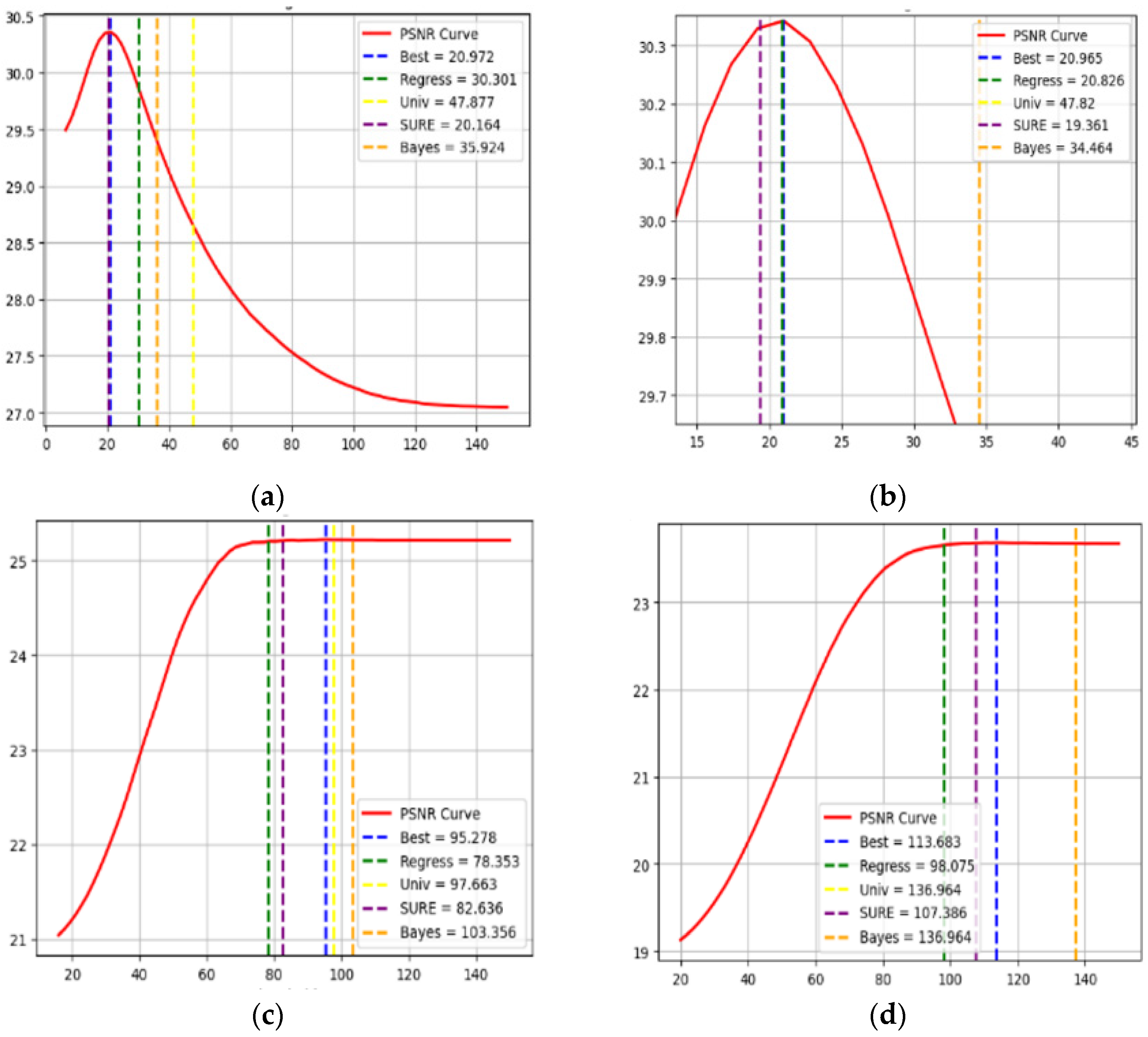
where λ represents the threshold, x_HH denotes the wavelet coefficients containing high-frequency information in both the horizontal and vertical directions, and M × N is the image size. However, this method applies a relatively fixed threshold, which makes the denoising performance less robust. As demonstrated in subsequent experiments, its effectiveness is often suboptimal. To address this limitation, we employed a regression analysis approach to explore the relationship between the median of wavelet coefficients and the optimal threshold for a more robust denoising performance.

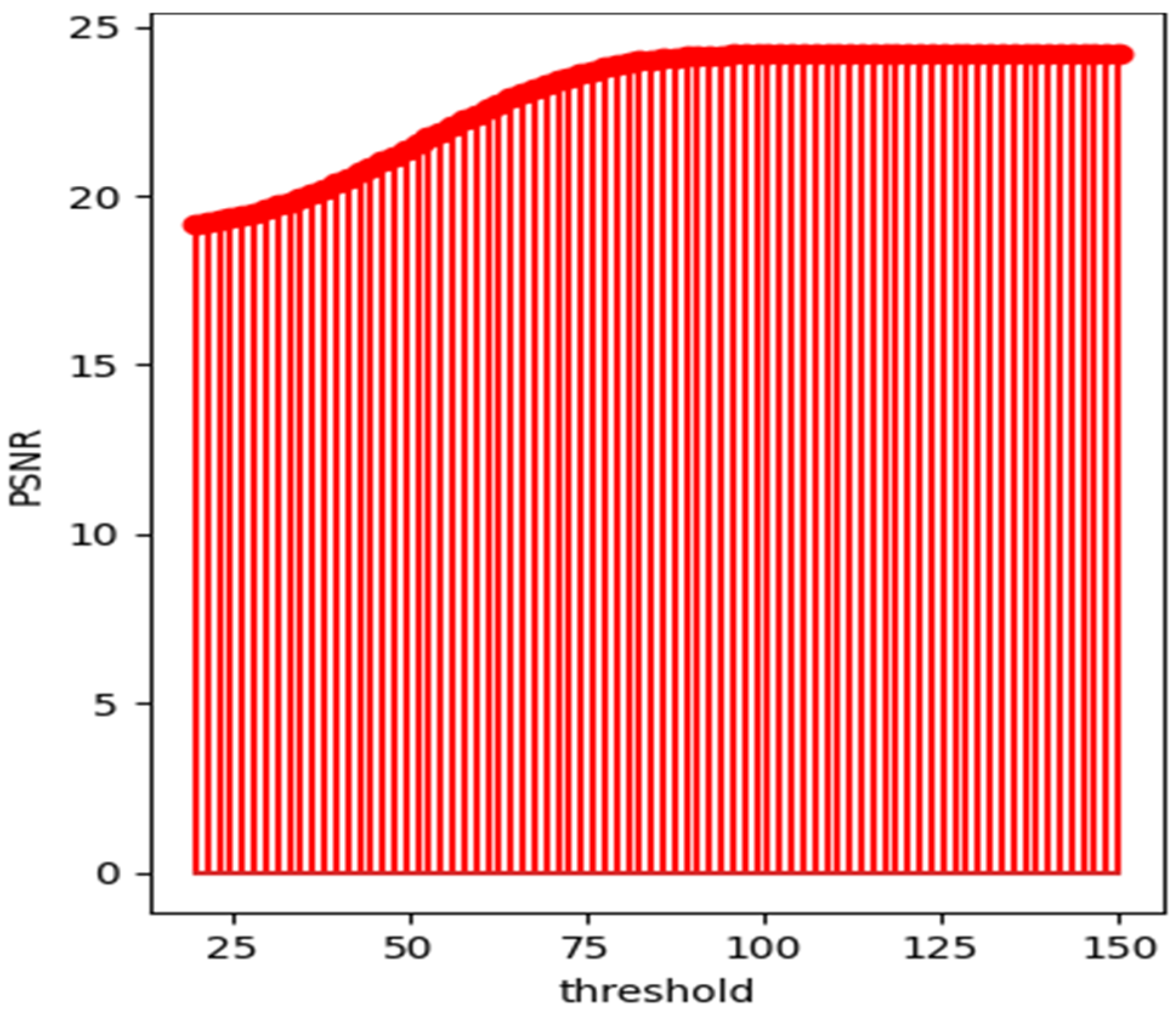
By applying wavelet thresholding denoising with various threshold values, we observed that the relationship between the threshold and PSNR follows an S-curve (Figure 1). When the denoising performance reaches its optimal limit, increasing the threshold does not improve PSNR; instead, it deteriorates the image by removing more essential details. Based on this observation, we collected the threshold values at which PSNR reaches its peak and no longer exhibits significant variation, considering them as the most appropriate thresholds. This process yielded a set of data pairs consisting of appropriate thresholds and the median of wavelet coefficients. In other words, we systematically tested various thresholds on noisy images and recorded the corresponding PSNR after denoising. When PSNR stabilized without significant improvement, we selected the corresponding threshold as the optimal one.

To refine this process, we generated a large dataset by applying this method to multiple noisy images. Using these data pairs, we applied regression analysis with the least-squares method to derive a regression line that models the relationship between the appropriate threshold and the median of wavelet coefficients. The mathematical formulation is as follows:

$$A=\left[\begin{array}{ccc}{m}_1& & 1\\ ⋮& & ⋮\\ m_n& & 1\end{array}\right],b=\left[\begin{array}{c}{t}_1\\ ⋮\\ t_n\end{array}\right],x=\left[\begin{array}{c}{x}_1\\ x_2\end{array}\right],$$

(2)

$$A^{T}Ax=A^{T}b,$$

(3)

$$=>x={\left(A^{T}A\right)}^{-1}{A}^{T}b$$

(4)

where A is a n × 2 matrix, b is a n × 1 vector, x is a 2 × 1 vector, $m_i$ represents the median of the wavelet coefficients for the ith noisy image, $t_i$ denotes the corresponding optimal threshold, $x_1$ is the slope of the regression line, and $x_2$ is the y-intercept.

By utilizing the least-squares method with n samples, we obtained a regression line for a more accurate estimation of the threshold. In processing images with high noise levels, many conventional methods select excessively large thresholds, which severely degrade image details. In contrast, the developed method in this study, based on appropriate thresholds derived from real samples, better balances between noise removal and the preservation of original image features.

Next, we identified the regression line for images of different sizes and investigated whether the regression line exhibits variations between large and small images. As the image size increased, the slope of the regression line was reduced, which led to a more appropriate threshold. Based on the results, we developed an adaptive thresholding method that adjusts according to image size. The mathematical formulation is as follows:

$$\lambda =\left\{\begin{array}{c}4.75\ast med\left({|x}_{HH}|\right),ifMN>512\ast 512\\ \left(5.15-{\displaystyle \frac{0.1MN}{256\ast 256}}\right)med\left(\left|x_{HH}\right|\right),if512\ast 512>MN>256\ast 256\\ \begin{array}{c}\left(5.45-{\displaystyle \frac{0.1MN}{128\ast 128}}\right)med\left(\left|x_{HH}\right|\right),if256\ast 256>MN>128\ast 128\\ \begin{array}{c}\left(5.75-{\displaystyle \frac{0.1MN}{64\ast 64}}\right)\ast med\left(\left|x_{HH}\right|\right),if128\ast 128>MN>64\ast 64\\ 5.65\ast med\left({|x}_{HH}|\right),ifMN<64\ast 64\end{array}\end{array}\end{array}\right.$$

(5)

where med$\left({|x}_{HH}|\right)$ is a median function, and M × N represents the size of the wavelet coefficients, meaning that the effective size is one-fourth of the original image size.

This adaptive threshold enables the selection of an appropriate threshold across different conditions. The threshold is used to achieve the highest PSNR. However, PSNR can be lowered with a lower threshold, which helps preserve more image details. We discovered a common limitation shared by many threshold selection methods: when an image is affected by low-level noise, the selected threshold tends to be too high. In such cases, over-thresholding significantly impacts PSNR, even resulting in worse performance than without denoising. Therefore, we refined the developed threshold selection method to determine the optimal threshold even in the presence of low-level noise.

2.2. Improved Threshold Based on Low-Noise Conditions

In low-noise conditions, the threshold tends to be overestimated, significantly reducing the effectiveness of wavelet threshold denoising. To address this, we improved previous methods by introducing a decay factor to adjust the slope of the regression line, ensuring a more appropriate threshold selection. However, a new challenge exists as the slope reduction rate must be decided. To determine this, we replaced the dataset used in the previous regression analysis with a collection of low-noise images and then recomputed the regression line. This allowed us to obtain the precise slope required for low-noise conditions. Once the appropriate slope reduction was determined, we used the median of wavelet coefficients as an indicator of noise magnitude. Based on this estimation, we computed the decay factor accordingly. The final mathematical formulation is as follows:

$$D=\left\{\begin{array}{c}-2\ast e^{-{\displaystyle \frac{\left(med\left(x_{HH}\right)-5.5\right)}{3}}}if|med\left(x_{HH}\right)|\ge 5.5\\ 0.5\ast med\left(x_{HH}\right)-4.75if\left|med\left(x_{HH}\right)\right|<5.5\end{array}\right.$$

(6)

where D is the decay factor, and med$\left({|x}_{HH}|\right)$ is the median function, which is added to the slope of our proposed adaptive threshold to flatten it under low-noise conditions, while the noise level is determined using the median of wavelet coefficients.

When the noisy image contains almost no noise, the median wavelet coefficient approaches 1, causing the decay factor to reduce the slope to nearly zero. As a result, the threshold value also approaches zero, ensuring that when no noise is present, no wavelet coefficients are removed. Second, as the noise level increases, the decay factor gradually decreases, and when the median wavelet coefficient reaches 5.5, the decay factor is set to −2, a value derived from regression analysis. This adjustment helps select the optimal threshold. Third, once the median wavelet coefficient exceeds 5.5, the decay factor rapidly decreases to zero, reverting to the original adaptive threshold formulation. This design allows the threshold to effectively adjust based on noise levels.

2.3. Improved Threshold Based on Multiresolution

When using multiresolution, the threshold for denoising deeper wavelet coefficients must be decreased [8]. This is reasonable, as the deep layers of wavelet coefficients tend to become more biased toward low frequencies, which are typically the signal components rather than the noise. Therefore, reducing the number of wavelet coefficients to be removed and lowering the threshold is also inevitable.

$${\lambda }_N={\displaystyle \frac{\lambda }{{\left(e^{\left(-1+1/N\right)}+\ln \left(N+1\right)\right)}^{1/2}}},N\ge 2$$

(7)

where ${\lambda }_i$ is the threshold used for the wavelet coefficients at the ith level, and N represents the number of levels to which the image is decomposed.

2.4. Improved Wavelet Denoising Algorithm

We integrated the improved methods into an algorithm to enhance wavelet threshold denoising. The algorithm enables the selection of the most appropriate threshold for any noise level and effective noise removal while preserving image details. Due to this advantage, the algorithm is well-suited for denoising algorithms, such as block-matching and 3d filtering (BM3D) [9], BM3D_DWT [10], and other wavelet-based denoising methods [11]. This algorithm addresses the issue of inaccurate matching when the image noise is too high. 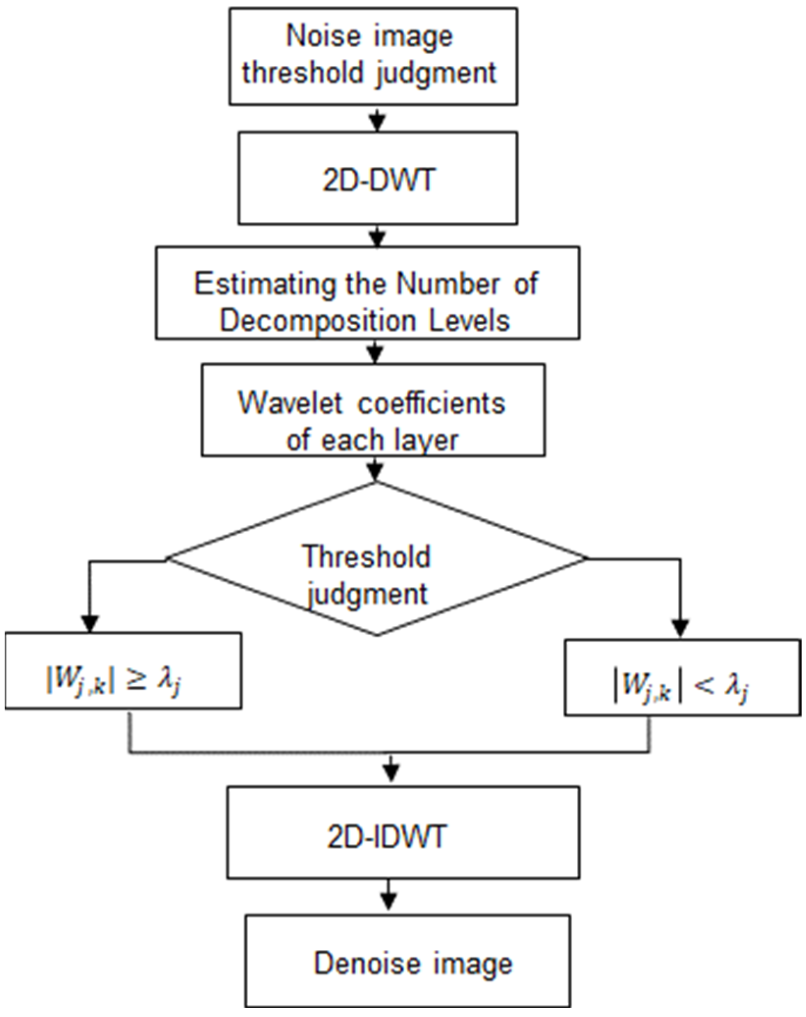Figure 2 illustrates the flowchart of this algorithm.

Due to the characteristics of noise, the amount of noise removed from the spatial domain is limited. Therefore, the wavelet transform was employed to convert noisy images into the wavelet domain for processing. Noise and signals exhibit different characteristics. Signal components in the wavelet domain typically have larger coefficients, while noise components, with low correlation with the signal, tend to have smaller coefficients. By applying a threshold to remove small wavelet coefficients and then transforming the processed wavelet coefficients back to the familiar spatial domain, noise can be effectively removed. Therefore, we considered multiple decompositions in the denoising algorithm developed in this study.

The noisy image is transformed into the wavelet domain using two-dimensional discrete wavelet transform (2D-DWT), obtaining the first-level wavelet coefficients: low-frequency component (x1_LL), high-frequency component in the horizontal direction (x1_LH), high-frequency component in the vertical direction (x1_HL), and high-frequency component in both horizontal and vertical directions (x1_HH). The first-level low-frequency sub-band, x1_LL, is then further decomposed into relatively low-frequency and high-frequency components, generating the second-level wavelet coefficients (x2_LL, x2_LH, x2_HL, and x2_HH). This process is recursively applied to further decompose x2_LL, fully utilizing the multiresolution property of the wavelet transform. As a result, an appropriate number of decomposition levels is selected, and for each level, an optimal hard threshold is applied to remove noise from the wavelet coefficients. The denoised wavelet coefficients from the (n + 1)th level are combined to form the low-frequency subband of the nth level. This process is repeated until the final denoised image is reconstructed (Figure 1).

3. Results

Experiments and simulations were conducted using Python 3.9 in this study. The wavelet basis used in all cases was db8, and the thresholding function applied was hard thresholding. The regression analysis was conducted using samples from nine different images, each with nine different levels of noise added, resulting in 81 sample points. To ensure that variations in image texture did not affect the experimental results, a diverse set of images was used to compute the regression line. The PSNR calculation formula is as follows:

$$\mathrm{P}\mathrm{S}\mathrm{N}\mathrm{R}=10\ast \mathrm{l}\mathrm{o}\mathrm{g}({\displaystyle \frac{{255}^2\ast MN}{\sum \sum {\left(\widehat{I}\left(x,y\right)-I\left(x,y\right)\right)}^2}})$$

(8)

where $MN$ is the image size, $\widehat{I}\left(x,y\right)$ is the processed image, and $I\left(x,y\right)$ is the original image. We use PSNR as the evaluation metric for image quality, with higher values indicating better quality.

In Figure 1, the star markers indicate the selected appropriate thresholds, which are not necessarily the thresholds that yield the highest PSNR. Because increasing the threshold further did not significantly improve PSNR, we chose the star positions and the wavelet coefficient median as a sample pair to select a slightly smaller threshold while achieving a similar denoising effect. Here, we defined the appropriate threshold as the point where PSNR growth is less than 0.01. Next, we used 81 sample pairs to compute the regression lines and tested image sizes of 1024 × 1024, 512 × 512, 256 × 256, and 128 × 128, resulting in four regression lines (

Table 1. Slopes of four regression lines.

	10242	5122	2562	1282
$x_1$	4.71	5.13	5.29	5.6
$x_2$	5.50	−1.87	−3.919	1.36

). We disregarded the intercepts and, since images were not limited to these specific sizes, we linearly interpolated the slopes of the four regression lines. This approach ultimately led to an adaptive thresholding method based on image size.

To address the issue of inaccurate threshold selection in low-noise conditions, we modified the experimental samples by using the same nine images but introducing only low-level noise. This setting enabled a more precise observation of slope behavior in low-noise environments. When the image was affected by low noise, the median of the wavelet coefficients decreased. Therefore, we selected the median of the wavelet coefficients as an indicator to estimate the noise level in the image. When the median of the wavelet coefficients was 5.5, the slope was reduced by 2 to obtain an appropriate threshold. When the image contained no noise, the slope was reduced to 0, and we conducted linear interpolation to connect these two key points. Moreover, as noise levels increased, we employed the exponential function to rapidly decrease the decay factor to 0 to ensure a reasonable threshold selection.

4. Discussion

We compared the method of this study with other existing threshold selection methods. In Figure 3, the red line represents the PSNR obtained using a given threshold for wavelet denoising, the blue line represents the optimal threshold, the green line represents our method, the yellow line represents VisuShrink [1], the orange line represents BayesShrink [2], and the purple line represents SureShrink [3]. In Figure 3a, the case without the noise is shown. The cases of low noise, moderate noise, and high noise are shown in Figure 3b, 3c, and 3d, respectively. Before applying the decay factor, the method developed selected a relatively large threshold. However, in low-noise conditions, choosing an excessively large threshold even degraded the PSNR beyond the original value, indicating the necessity for improvement. After applying the decay factor and zooming in on the image, the selected threshold was reduced, making it closer to the optimal threshold and the closest compared with those of previous methods (Figure 3b). In moderate and high noise conditions, we selected an “appropriate” threshold.

Although the threshold is not the closest to the optimal threshold, the developed method sacrifices a nearly negligible amount of PSNR to achieve a significantly smaller threshold, to better preserve image details. We tested the method across various image sizes and found it to be highly competitive in all cases. The most competitive alternative is SureShrink, but it requires searching over a large range of thresholds and calculating risk, leading to significantly higher computational complexity than the developed method. VisuShrink and BayesShrink consistently select excessively large thresholds, resulting in the loss of important details.

Table 2. Average values of optimal decomposition levels based on image size and median of wavelet coefficients, which can be used to estimate the optimal decomposition level.

	med$\left(\right|{\mathit{x}}_{\mathit{H}\mathit{H}}|$)	4	7	10	13	15	18	21	24	27
Size
10242		1.77	2	2.11	2.22	2.78	2.89	3.00	3.00	3.56
5122		0.89	1.22	1.78	2.00	2.11	2.33	2.78	2.89	3.56
2562		0.89	1.00	1.78	2.11	2.44	2.67	3.67	2.89	3.45
1282		0.89	1.00	1.56	1.89	2.22	2.67	3.22	3.00	3.33

presents the average values of the optimal decomposition levels based on image size and the median of the wavelet coefficients. This can be applied to estimate the optimal decomposition level.

5. Conclusions

In this study, we addressed the challenge of threshold selection using regression analysis by determining the most appropriate threshold rather than the optimal one to achieve a balanced trade-off between noise removal and detail preservation. We refined the developed method by introducing a slope decay factor for low-noise images and optimizing the number of decomposition levels to fully utilize the multiresolution properties of wavelets. Experimental results demonstrate that the developed method effectively adapts threshold selection based on noise level and image size, making it superior to classical methods. Its superior balance between noise reduction and detail preservation makes its preprocessing fit various denoising algorithms. It is still necessary to enhance the robustness and efficiency of the algorithm and improve the thresholding function beyond hard thresholding for better denoising performance.