Improving Effectiveness of Energy Baseline Using Deep Learning ^†

Abstract

Energy conservation and carbon reduction are critical in energy policies. Therefore, numerous energy-saving methods, such as the introduction of new technologies and the replacement of outdated equipment, have been proposed. To determine whether these methods are effective in energy conservation and carbon reduction, scientific validation is required. The most common validation method is energy baseline. An energy baseline refers to the use of data measured before energy-saving improvements. It is used to construct a mathematical model that describes energy consumption. Using the baseline, the energy consumption during the baseline period after improvements is calculated. By subtracting the measured consumption from the value, the amount of energy saved is estimated. Traditionally, linear regression is used to establish energy baseline prediction. However, linear regression has limitations with complex energy data. Therefore, we used deep learning models to handle nonlinear data in the air compression system for comparative analysis. The developed long-short-term memory (LSTM) model showed superior capabilities for processing nonlinear data, aligning with the actual data distribution, and reducing errors. Compared with linear regression models, the LSTM model reduced uncertainty, risk, and cost by 40.3%.

1. Introduction

Energy conservation and carbon reduction are crucial in energy policies. Various energy-saving methods, such as those involving the introduction of new technologies and the replacement of outdated equipment, have been proposed. However, a scientific method is required to verify the effectiveness of these methods in achieving energy conservation and carbon reduction with the establishment of energy baselines.

An energy baseline in a mathematical model is used to describe energy consumption using data measured before energy-saving improvements. Energy baselines are also used to estimate baseline energy consumption after improvements. The differences between the estimated baseline consumption and the measured consumption represent the energy saved using the improvement methods [1]. Currently, the most commonly used mathematical model for establishing energy baselines is the linear regression model. This model is simple and easy to use, and it facilitates rapid computation. However, it often fails to accurately fit when processing complex data. Therefore, a mathematical model with higher energy baseline fit performance must be developed to enable precise comparisons of energy consumption before and after the implementation of energy-saving measures, facilitate accurate assessments of the effectiveness of energy-saving methods, and provide a more convincing basis for energy-saving decisions. In this study, we focused on the air compressor system at a specific site.

The rest of this paper is arranged as follows. Section 2 introduces the linear regression model and the operational principles of the long-short-term memory (LSTM) network. Section 3 describes the examined air compressor system, and Section 4 details the simulations and comparative analyses conducted in this study. Finally, Section 5 provides the conclusions of this study. According to the simulation results of this study, deep learning is a more suitable method for establishing energy baselines.

2. Energy Baseline Model

Linear regression and deep learning methods were used to establish energy baselines in this study. An energy baseline model and optimal model parameters were constructed under the assumption that a dataset [i.e., (X_n, Y_n), where X ∈ R^m and Y ∈ R] contains n pieces of data and m features.

2.1. Linear Regression

The linear regression equation for the aforementioned dataset is expressed as follows [2]:

$$\mathit{Y}=\mathit{X}\mathit{\beta }+\mathit{\epsilon }$$

(1)

$$\mathit{Y}=\left[\begin{array}{c}{Y}_1\\ ⋮\\ Y_n\end{array}\right],\mathit{\beta }=\left[\begin{array}{c}{\beta }_0\\ ⋮\\ \beta m\end{array}\right],\mathit{X}=\left[\begin{array}{ccc}1& X_{11}& \begin{array}{cc}\dots & X_{1m}\end{array}\\ ⋮& ⋮& \begin{array}{cc}\ddots & ⋮\end{array}\\ 1& X_{n1}& \begin{array}{cc}\dots & X_{nm}\end{array}\end{array}\right],\mathit{\epsilon }=\left[\begin{array}{c}{\epsilon }_1\\ ⋮\\ {\epsilon }_n\end{array}\right]$$

(2)

where $\mathit{\beta }$ represents the parameters of the linear regression model, and ε is the error term [${\epsilon }_n~N(0,{\sigma }^2)$].

The loss function of the model is defined using the least squares method as follows:

$$Loss\left(\mathsf{\beta }\right)={\left(\mathbf{Y}-\mathbf{Y}\right)}^{\mathit{T}}(\mathbf{Y}-\mathbf{Y})$$

(3)

This loss function is rearranged and expressed as ${\mathit{Y}}^T\mathit{Y}+{\mathit{X}}^T\widehat{\mathit{\beta }}\widehat{\mathit{\beta }}\mathit{X}-2{\mathit{X}}^T\widehat{\mathit{\beta }}\mathit{Y}$. To find the optimal parameter β, the partial derivative of the loss function is taken to determine its extreme value.

$${\displaystyle \frac{\partial Loss\left(\mathit{\beta }\right)}{\partial \mathit{\beta }}}=0\Rightarrow \widehat{\mathit{\beta }}=({\mathit{X}}^T\mathit{X}{)}^{-1}{\mathit{X}}^T\mathit{Y}$$

(4)

2.2. LSTM Network

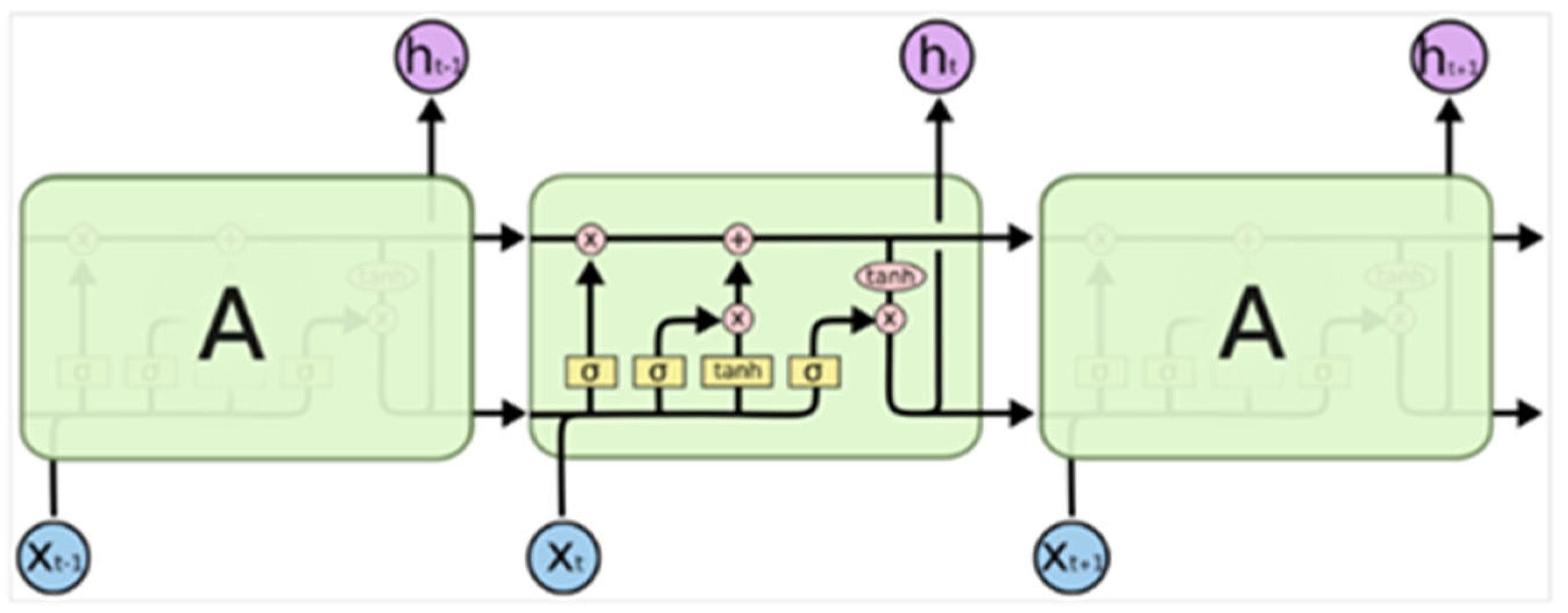
An LSTM network is an extension of a recurrent neural network (RNN) that addresses the limitations of RNNs in retaining memory and obtaining the optimal parameters [3,4]. An LSTM network consists of four main components: a cell state, a forget gate, an input gate, and an output gate. The structure of this network is shown in Figure 1.

In Figure 1, each rectangle with rounded edges represents an LSTM cell. The horizontal line running through all cells is the LSTM state, which is the main location where memory is stored. The memory state at time step t is denoted as $C_t$, which is updated from $C_{t-1}$ by discarding and adding information within the cell. The first $\sigma$ rectangle inside the cell is the forget gate, which is denoted as $f_t$ and determines the extent to which the information in the cell state $C_{t-1}$ should be discarded. The term $f_t$ is computed as follows:

$$f_t=\sigma (W_f\times {\mathit{X}}_t+U_f\times h_{t-1})$$

(5)

where W represents the weights of the input data, $h_{t-1}$ is the output at time t − 1 (corresponding to the arrow below the cell in Figure 1), and U is the weight of the previous time step’s output at time t − 1. Moreover, $\sigma$ is a sigmoid function, which has values between 0 and 1. The second $\sigma$ rectangle inside the cell represents the input gate, which is denoted as $i_t$ and determines the extent to which new input data $\widetilde{C_t}$ must be added. The values of the input gate also range from 0 to 1.

$$i_t=\sigma (W_i\times {\mathit{X}}_t+U_i\times h_{t-1})$$

(6)

The third rectangle inside the cell represents the input content, which is denoted as $\widetilde{C_t}$ and expressed as follows:

$$\widetilde{C_t}=\mathit{tanh}(W_c\times {\mathit{X}}_t+U_c\times h_{t-1})$$

(7)

The activation function of $\widetilde{C_t}$ is the hyperbolic tangent function (tanh).

As displayed in Figure 1, the memory state is updated through the memory gate and input gate. This update is expressed as follows:

$$C_t=f_t\times C_{t-1}+i_t\times \widetilde{C_t}$$

(8)

This equation represents the sum of the previous memory state multiplied by the forget gate and the new input content multiplied by the input gate. It describes the process of discarding a part of the old information while incorporating new information.

After the memory state is updated, $C_t$ is output through two pathways. The first pathway passes along the straight line that runs through all cells, with $C_t$ passing to the next cell at time step t + 1. The second pathway generates the output of the estimated value $\widehat{Y_t}$ at time step t, which is controlled by the output gate (denoted as $o_t$).

$$o_t=\sigma (W_o\times {\mathit{X}}_t+U_o\times h_{t-1})$$

(9)

The output information is represented as $h_t$, which is expressed as follows:

$$h_t=o_t\times \mathit{tanh}(C_t)$$

(10)

After $h_t$ is calculated, it must be passed to the output layer and the next time step t + 1. The output layer produces the desired label, and $\widehat{Y_t}$ is used to denote the estimated value at time step t.

$$\widehat{Y_t}=\sigma (W_h\times h_t)$$

(11)

Because the execution of an LSTM network involves time step computation, parameter optimization is conducted using the backpropagation through time (BPTT) algorithm, which combines traditional neural network backpropagation with the chain rule from calculus.

The loss function is defined using entropy. The loss function at time step t is as follows:

$$E_t(Y_t,\widehat{Y_t})=-Y_t\mathit{log}(\widehat{Y_t})$$

(12)

where $Y_t$ is the actual value and $\widehat{Y_t}$ is the predicted value. Although equations contain numerous parameters, an LSTM network benefits from weight sharing, meaning that the parameters $f_t$, $i_t$, $\widetilde{C_t}$, and $o_t$ essentially have the same value. Therefore, only three main parameters (i.e., $W_h$, $W_o$, and $U_o$) must be calculated. BPTT derivation is a complex and lengthy process; a more detailed explanation of this method can be found in [5].

3. Air Compressor System

An air compressor system was examined in this study. A schematic of this system is shown in Figure 2.

KW1 and KW2 are the power meters used to record the power consumption data of the air compressor system. These data include three-phase current, three-phase line voltage, power consumption, power factor, and total system energy consumption. Moreover, PT1 and PT2 are pressure gauges that measure pressure-related variables, including air tank pressure, system pressure, and differential pressure. Finally, FT1, FT2, and FT3 are flow meters that record gas-flow-related variables, such as fluid temperature, flow pressure, flow velocity, and flow rate.

To collect relevant energy consumption data from the air compressor system’s flow meters, pressure gauges, and power meters, the Pearson correlation coefficient was calculated for each variable with power consumption (kW) and energy consumption (kW/CMM). The variables are ranked by the descending order of their correlations in

Table 1. Power-consumption-related correlation coefficients.

Correlation coefficient	Flow rate (CMM)	Differential pressure (mBar)	Air tank pressure(Bar)	Output frequency (Hz)	System pressure (Bar)
	0.8594	0.8454	0.4049	0.3972	0.2365

and

Table 2. Energy-consumption-related correlation coefficients.

Correlation coefficient	Flow rate (CMM)	Differential pressure (mBar)	Air tank pressure(Bar)	Output frequency (Hz)	System pressure (Bar)
	0.4764	0.4763	0.3854	0.2982	0.2273

.

After the correlation coefficients were calculated and variables directly related to power consumption (i.e., current and voltage) were excluded, the results indicated that flow rate and differential pressure were highly correlated with power consumption, air tank pressure and output frequency were moderately correlated with power consumption, and system pressure had a low correlation with power consumption. The other variables were not correlated with power consumption.

Flow rate (CMM) represents the rate of gas flow in an air compressor system. The differential pressure (mbar) refers to the pressure difference across filters, as recorded by pressure gauge PT2. Air tank pressure (bar) is measured by pressure gauge PT1, and output frequency (Hz) represents the variable frequency data of the air compressor system. Finally, system pressure (bar) is the pressure value recorded by pressure gauge PT2.

4. Simulations and Results

Energy baselines established using deep learning methods enabled a model to better fit the data distribution characteristics compared with those derived from linear regression models. Power consumption (kW) and energy consumption (kW/CMM) were used as the prediction targets. The variables were highly correlated with the prediction targets selected as explanatory variables to construct the energy baseline model.

Data from October to December 2024 for an air compressor system at a specific site were selected as training data. Moreover, data from January 2025 for this system were selected as the test data. Model performance was evaluated using mean squared error (MSE) as follows:

$$\mathrm{MSE}={\displaystyle \frac{1}{n}}\sum _{i=1}^n(Y_i-\stackrel{⏜}{Y_i}{)}^2$$

(13)

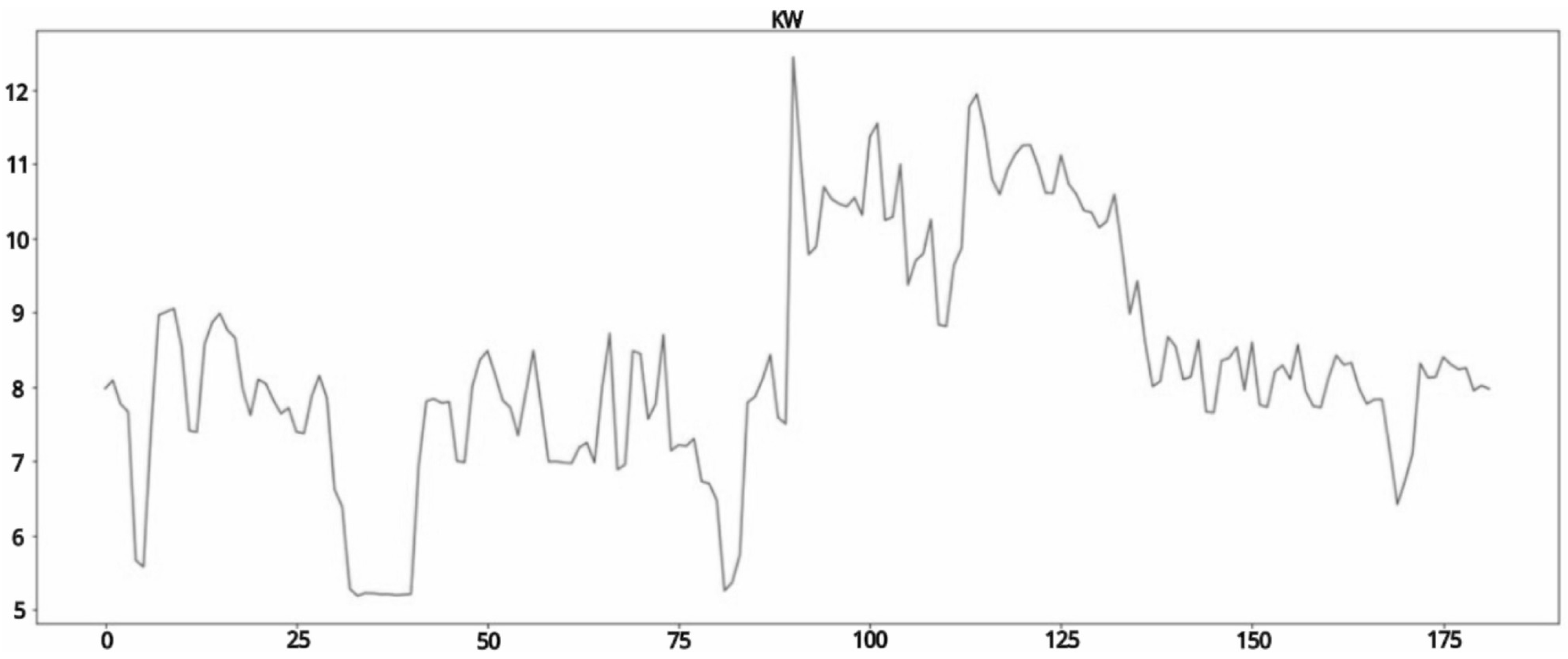
The descriptive statistics of the examined air compressor system were obtained for flow rate, differential pressure, air tank pressure, and output frequency, denoted as $\left\{\right({\mathit{X}}_n^{train1},Y_n^{train1}\left)\right|{\mathrm{X}}_{\in }{\mathbb{R}}^4,{\mathrm{Y}}_{\in }\mathbb{R},n=\left.\mathrm{1,477,470}\right\}$, to predict power consumption. Figure 3 illustrates the power consumption scatterplot, in which the x-axis represents days, and the y-axis represents daily average power consumption values. Because the dataset was large, the scatterplot was created using daily average values to ensure readability.

Table 3. Descriptive statistics for power consumption.

Statistical Measure	Mean	Standard Deviation	Maximum Value	Minimum Value
Value	8.4029	4.5918	28.3	1.4

presents the descriptive statistics for power consumption.

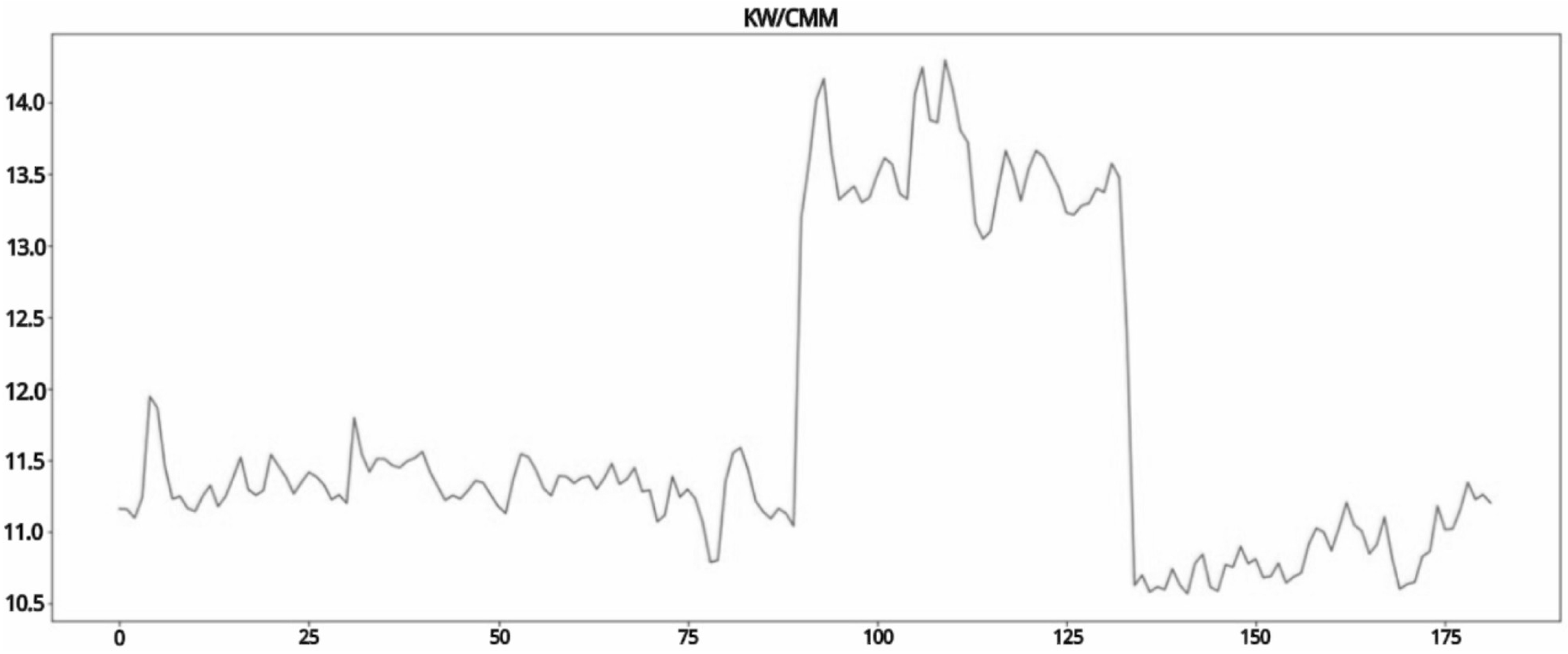
Flow rate, differential pressure, and air tank pressure, denoted as $\left\{\left(X_n^{train2},Y_n^{train2}\right)|X_{\in }{\mathbb{R}}^3,Y_{\in }\mathbb{R},n=\left.\mathrm{1,477,470}\right\}\right.$, were selected to predict energy consumption. Figure 4 illustrates the energy consumption scatterplot, and

Table 4. Descriptive statistics for energy consumption.

Statistical Measure	Mean	Standard Deviation	Maximum Value	Minimum Value
Value	11.748	3.9118	53	1.56

presents the descriptive statistics for energy consumption.

Next, $\left\{\left(X_n^{test1},Y_n^{test1}\right)|X_{\in }{\mathbb{R}}^4,Y_{\in }\mathbb{R},n=\left.\mathrm{163,869}\right\}\right.$ was used to represent the test data for power consumption, whereas $\left\{\left(X_n^{test2},Y_n^{test2}\right)|X_{\in }{\mathbb{R}}^3\right.$ was used to represent the test data for energy consumption. Figure 5 and Figure 6 show the scatterplots for the test data on daily average power consumption and daily average energy consumption, respectively.

Linear regression and LSTM models were used to establish baselines for the power consumption of the examined air compression system. The simulation results are described as follows.

Table 5. Numerical simulation results obtained for power consumption by using the linear regression and LSTM models.

Model	Linear Regression	LSTM
MSE	4.8533	2.8047

presents the numerical simulation results obtained with the linear regression and LSTM models for power consumption. The performance of the linear regression model was inferior to that of the LSTM model, making the linear regression model unsuitable for evaluating the effectiveness of energy-saving methods. Although the LSTM model produced a smaller error than did the linear regression model, a notable drawback of deep learning models is that they must conduct numerous computations, leading to a long simulation time. Therefore, we also calculated the computation times of both models in the power consumption simulations (

Table 6. Computation times of the linear regression and LSTM models in power consumption simulations.

Model	Linear Regression	LSTM
Training time	0.25(s)	4383(s)
Test time	0.007(s)	3.399(s)

).

The training and testing times for both models were calculated. The linear regression model was considerably faster than the LSTM model in the training process. However, both models exhibited short testing times. Therefore, the LSTM model exhibited a more favorable overall performance than the linear regression model in the establishment of energy baselines for evaluating the effectiveness of energy-saving methods.

The linear regression and LSTM models were also used to establish baselines for the energy consumed by the air compression system.

Table 7. Numerical simulation results obtained for energy consumption by using the linear regression and LSTM models.

Model	Linear Regression	LSTM
MSE	10.6136	6.3364

presents the numerical simulation results obtained with these models for energy consumption. The linear regression model exhibited inferior performance, likely because of the weak linear relationships of the explanatory variables with energy consumption, as indicated by the low correlation coefficients. The LSTM model considerably outperformed the linear regression model because deep learning models are well-suited for processing nonlinear data.

Table 8. Computation times of the linear regression and LSTM models in energy consumption simulations.

Model	Linear Regression	LSTM
Training time	0.25(s)	2315(s)
Test time	0.007(s)	2.149(s)

presents the calculation times of both models in the energy consumption simulations. The results in Table 8 are consistent with those in Table 6. The linear regression model again exhibited a considerably shorter training time than the LSTM model. However, both models exhibited short testing times. Therefore, the LSTM model is more suitable to the linear regression model for establishing energy baselines to evaluate the effectiveness of energy-saving methods.

5. Conclusions

We conducted empirical analyses to compare the performance of linear regression and LSTM models in establishing energy baselines. The results indicated that the LSTM model provided more accurate energy baselines than the linear regression model, which is commonly used for energy-saving evaluations. The performance of the linear regression model was hindered when it processed nonlinear data, resulting in poor model fitting. Consequently, decision-makers using this model might struggle to make accurate energy-related decisions, and they fail to accurately determine the effectiveness of energy-saving methods. Conversely, the LSTM model exhibited a strong capability to process nonlinear data and generated models that accurately aligned with the actual data distribution. Consequently, the LSTM model showed lower error rates in energy consumption prediction, being more appropriate for establishing energy baselines than the linear regression model. The LSTM model reduced uncertainty, risk, and cost by 40.3% compared with traditional regression models.