A Forecasting Method Based on a Dynamical Approach and Time Series Data for Vehicle Service Parts Demand ^†

Abstract

In the automotive industry, the supply of service parts—such as bumpers, batteries, and aero parts—is required even after the end of vehicle production, as customers need them for maintenance and repairs. To earn customer confidence, manufacturers must ensure timely availability of these parts while managing inventory efficiently. An excess of inventory can increase warehousing costs, while stock shortages can lead to supply delays. Accurate demand forecasting is essential to balance these factors, considering the changing demand characteristics over time, such as long-term trends, seasonal fluctuations, and irregular variations. This paper introduces a novel method for time series forecasting that employs Ensemble Empirical Mode Decomposition (EEMD) and Dynamic Mode Decomposition (DMD) to analyze service part demand. EEMD decomposes historical order data into multiple modes, and DMD is used to predict transitions within these modes. The proposed method demonstrated an approximately 30% reduction in forecasting error compared to comparative methods, showcasing its effectiveness in accurately predicting service parts demand across various patterns.

1. Introduction

Service parts play an important role in the sustainable life of vehicles. In the automotive industry, the supply of service parts—such as bumpers, batteries, and aerodynamic parts (see Figure 1a)—is required even after the end of vehicle production, as customers need them for maintenance and repairs. For manufacturers, it is essential to provide a timely supply of service parts not only for regular maintenance but also for parts that need to be replaced due to accidents [1]. However, if service parts are out of stock when a failure occurs, repairs cannot be conducted until the parts are procured. To gain customer confidence, it is necessary to estimate the adequate quantity of service parts in advance and maintain a safe inventory level. On the other hand, if too much stock is held to mitigate the risk of shortages, it can lead to excess inventory, resulting in high maintenance costs and putting pressure on warehouse space. Therefore, it is crucial to estimate actual orders through demand forecasting to prevent both the risk of stockouts and the high costs associated with excess inventory, thereby maintaining appropriate inventory levels.

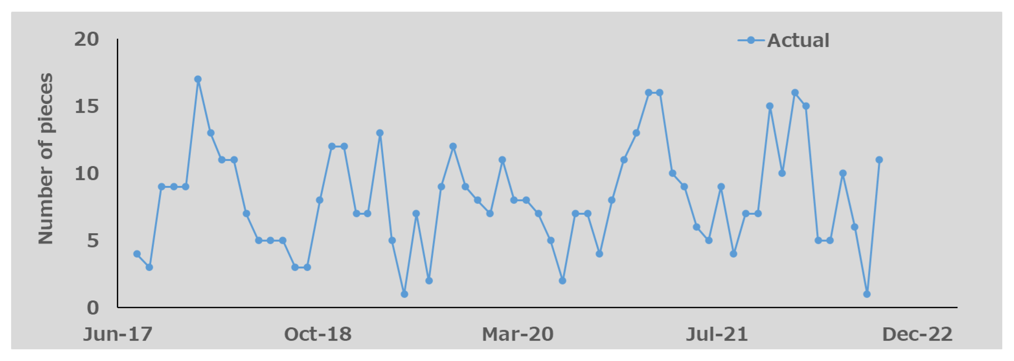
Service parts are essential for customers who wish to use their vehicles for a long time. Therefore, it is necessary to prepare for customer demand not only during vehicle production but also afterward, as maintenance may last over ten years after the product launch. Consequently, long-term changes in demand characteristics must be considered in the demand forecasting of service parts. The demand for these parts varies over their life cycle, with different characteristics in the early, middle, and late stages (see Figure 1b). Additionally, from a short-term perspective, the demand for service parts exhibits periodic fluctuations, such as seasonal changes, along with long-term variations. Therefore, to accurately predict the demand for a specific part, it is necessary to consider its historical order data.

In traditional inventory management, basic forecasting methods based on the quantity and frequency of historical service part orders are implemented using simple moving average or exponential smoothing [2,3]. While these methods are straightforward and widely used due to their ease of understanding and operation, they struggle to deliver sufficient accuracy for parts with significant seasonal fluctuations and high order variability. As a result, in practice, logistics staff have to carefully monitor the forecast values for certain parts that have experienced stockouts in the past and adjust them as necessary based on their own know-how. Due to this, dealing with a large number of parts that exhibit significant demand variability poses a challenge, as traditional methods may incur high costs in order to obtain safe inventory levels.

To overcome accuracy issues, the establishment of an effective forecasting method for various demand patterns is required. There are a number of time series forecasting methods based on statistical approaches, including the previously mentioned simple moving average and exponential smoothing. Autoregressive (AR) models [4] estimate future values based on a linear combination of past observations. In addition, combinations of moving averages, integral processes, and seasonal components have led to the proposal of autoregressive moving average (ARMA), autoregressive integrated moving average (ARIMA), and seasonal autoregressive integrated moving average (SARIMA) models [5]. However, all models are based on different assumptions about the nature of the underlying time series data; thus, their effectiveness is limited to specific applications. Recently, neural networks have emerged as a powerful alternative to these statistical approaches in time series forecasting [6]. Moreover, deep learning methods such as recurrent neural networks (RNNs) [7] and long short-term memory networks (LSTM) [8] have been extensively developed, with reports of deep learning models achieving higher accuracy compared to traditional models. On the other hand, deep learning forecasting models often have a large number of parameters and require substantial amounts of training data. Additionally, as the volume of training data increases, so does the time needed for training, making it difficult to maintain long-term dependencies [9]. Therefore, careful model selection is necessary for time series with such characteristics.

In this paper, a new forecasting method that can handle small univariate time series data with reliable accuracy, such as monthly historical orders of a single service part over several years, in predicting a wide range of demand patterns is proposed using Ensemble Empirical Mode Decomposition (EEMD) [10] and Dynamic Mode Decomposition (DMD) [11]. EEMD and DMD are, respectively, utilized to adaptively decompose arbitrary time series that change at different time scales into multiple Intrinsic Mode Functions (IMFs) and to represent the dynamics of the time series in each mode. In the proposed method, the order history of a single service part is decomposed into modes using EEMD. Subsequently, corresponding state variables for each mode are computed, and the transition prediction for each mode is conducted using DMD. Finally, the sum of the transition predictions is calculated as the demand forecast value for the individual part.

This paper is organized as follows: In the next section, the theoretical derivations of the proposed method, based on a dynamical approach, are described. The validation method using historical order data of service parts is presented in the third section. The fourth section discusses the validation results. In the last section, the benefits and limitations of the proposed method, as well as future work, are summarized.

2. Theoretical Backgrounds

To accurately forecast various demand patterns of service parts that change complexly over time, the forecasting model should ensure accuracy not only within the range of available historical order data (interpolation range) but also in the range where no training data exists (extrapolation range). Existing forecasting methods utilizing common statistical and machine learning techniques often face the challenge of ‘extrapolation’ [12]. In this section, a forecasting method is proposed to deal with the difficult task of ‘extrapolative forecasting’, drawing inspiration from dynamical systems. 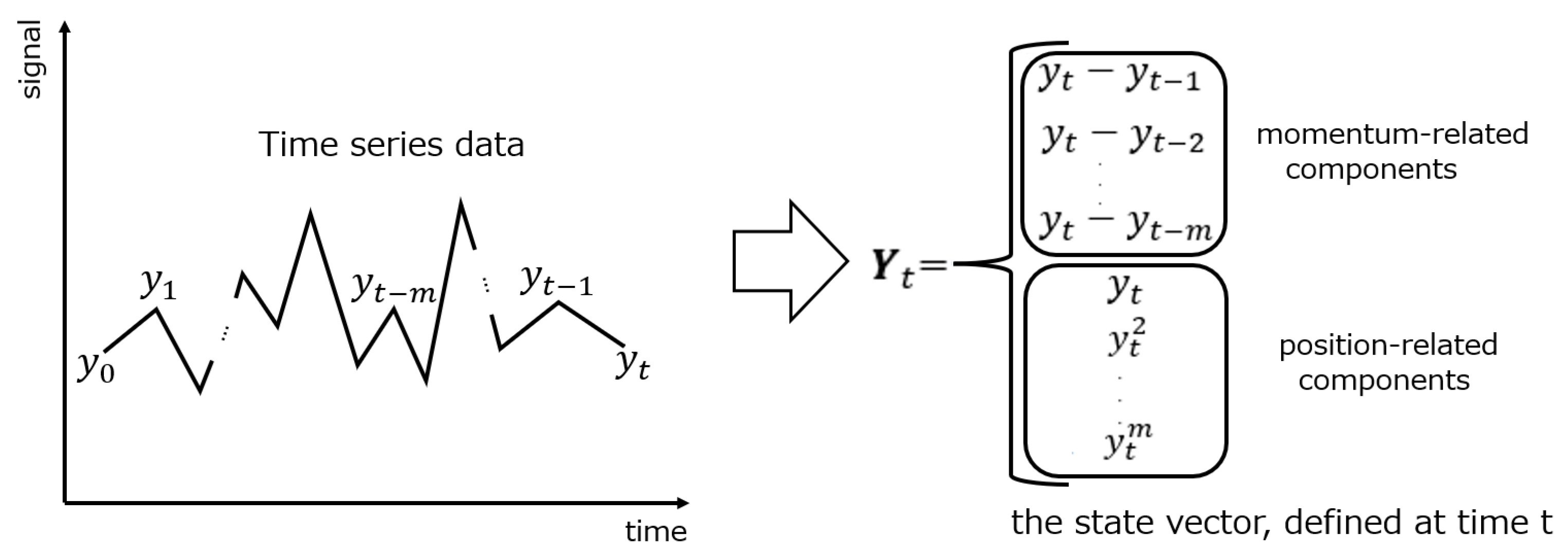As shown in Figure 2, in a dynamical system, the future states of the rolling motion of a ball can be determined by using information about its previous position and momentum under a governing equation, such as the Euler–Lagrange equation [13]. In time series data, if we can define the information of state variables corresponding to position and momentum at each time point from the time series data and can also simulate the laws of transition for such state variables at each time point, it will become possible to estimate the future states in a manner similar to dynamical systems.

This section describes a new formulation of state variables for time series data. To represent the law of transition for state variables, the theoretical background of the Koopman operator and the algorithm for DMD [14] are introduced, and a new formulation for demand forecasting based on this theory is established. Forecasting trials using test functions are also conducted to confirm the validity of the theories. Finally, EEMD and its applications are utilized to enhance forecast accuracy.

2.1. Formulation of State Variables

This subsection discusses state variables that represent time series dynamics and derives formulations for the position-related and momentum-related components that constitute these state variables from time series information. First, in the formulation of the position-related components, the observation of an analytic function $f$ applied to the signal $y_t$ at time $t,$ denoted as $f\left(y_t\right),$ can be approximated by a polynomial in $y_t$. Therefore, as shown in the following Equation (1), the observation can be represented as the inner product of a vector formed from the powers of the signal $y_t$ and a constant vector composed of the coefficients of the polynomial.

$$\begin{array}{c}f\left(y_t\right)=a_0+a_1{y}_t+a_2{y_t}^2+\dots +a_m{y_t}^m+\dots \\ \approx a_0+a_1{y}_t+a_2{y_t}^2+\dots +a_m{y_t}^m=\text{< }\mathit{a},{\mathit{y}}_{\mathit{t}}>,\end{array}$$

(1)

where the constant vector $\mathit{a}$ = ($a_0$, $a_1$ $\dots$, $a_m)$ and the coefficient $m$ denote the inherent information of the observation function $f$ and the truncation order of the approximation in Equation (1), respectively. Since the vector ${\mathit{y}}_{\mathit{t}}$ = $\left(y_t,y_t^2,\dots ,y_t^m\right)$ is analogous to the coordinate information of a position $\left(x,y,z\right)$ in three-dimensional space, it can be considered as the position-related vector in a multidimensional space generated by the signal $y_t$.

On the other hand, in the formulation of the momentum-related components, the calculation is performed using the difference in position-related vectors between the current time $t$ and the previous time $t-1$ as shown in Equation (2).

$$\begin{array}{l}(y_t-y_{t-1},y_t^2-y_{t-1}^2,\dots ,y_t^m-y_{t-1}^m)\\ \approx (y_t-y_{t-1},2y_{t-1}\times \left(y_t-y_{t-1}\right),\dots ,m{y}_{t-1}^{m-1}\times \left(y_t-y_{t-1}\right))\end{array}$$

(2)

After simplifying the above equation by removing the information regarding the powers of the signal $y_t$ that are already included in the position-related vector, the right side of Equation (2) can be written as follows.

$$\begin{array}{l}(y_t-y_{t-1},2y_{t-1}\times \left(y_t-y_{t-1}\right),\dots ,m{y}_{t-1}^{m-1}\times \left(y_t-y_{t-1}\right))\\ \to (y_t-y_{t-1},2\times \left(y_t-y_{t-1}\right),\dots ,m\times \left(y_t-y_{t-1}\right))\end{array}$$

(3)

Furthermore, using the approximation shown in the following Equation (4), the momentum-related components can be expressed as the difference between the current time signal $y_t$ and the past signals $y_{t-1},y_{t-2},\dots ,y_{t-m}$.

$$\begin{array}{c}2\times \left(y_t-y_{t-1}\right)\approx \left(y_t-y_{t-1}\right)+\left(y_{t-1}-y_{t-2}\right)=y_t-y_{t-2}\\ \dots \\ m\times \left(y_t-y_{t-1}\right)\approx \left(y_t-y_{t-1}\right)+\dots +\left(y_{t-m-1}-y_{t-m}\right)=y_t-y_{t-m}\end{array}$$

(4)

Therefore, as shown in Figure 3, state variables of the time series at each time $t$ can be represented as a vector consisting of the position-related components derived from the powers of $y_t$ and the momentum-related components formed by the difference between $y_t$ and the past signals $y_{t-1},y_{t-2},\dots ,y_{t-m}$.

2.2. Koopman Operator and Dynamic Mode Decomposition

To simulate time evolution of state variables mentioned in the previous subsection, we introduce here the theoretical backgrounds of Koopman operator and its numerical algorithm, Dynamic Mode Decomposition (DMD). The Koopman operator is an operator that describes the time evolution of observables in dynamical systems. It was introduced by Koopman in the 1930s, inspired by the development of quantum mechanics, in relation to the observables of classical Hamiltonian systems [15,16]. In the 21st century, discussions about the applications of the theory have been expanded by Mezić and others to include dissipative dynamical systems, significantly broadening the range of applicable subjects and leading to active research in fields such as applied mathematics and control theory [17,18,19]. Particularly in the field of fluid dynamics, a connection has been reported between data analysis of fluid motion, referred to as Dynamic Mode Decomposition (DMD), and the theory of the Koopman operator [20], and DMD has been widely applied to the analysis of fluid motion. The key point of the theory of dynamical systems using the Koopman operator is the introduction of a function space that fits well with the characteristics of the dynamical system and relates those characteristics to the properties of linear mappings acting on that function space.

This subsection outlines the global linearization of nonlinear dynamical systems using the Koopman operator and demonstrates the potential to characterize the time evolution of state variables based on the spectrum of the Koopman operator. First, we start with a discrete dynamical system described by the following equation.

$${\mathit{x}}_{t+1}=\mathit{F}\left({\mathit{x}}_t\right),$$

(5)

where $t$ represents discrete time, ${\mathit{x}}_t$ is the state vector at time $t$, and $\mathit{F}$ is a nonlinear mapping in the state space. Due to its nonlinearity, the computation and analysis for $\mathit{F}$ become difficult. In Koopman theory, a function $g$ is introduced as an observable, which maps from the state space $\mathit{X}$ to the complex number field $\mathbb{C}$, and the space formed by the set of functions $g$ is defined as the observable space $\mathcal{F}$. A mapping $\mathit{K}$, called the Koopman operator, that creates a new observable $g\circ \mathit{F}$ from the observable $g$ on the observable space $\mathcal{F}$, is defined as follows.

$$\left(\mathit{K}g\right)\left(\mathit{x}\right)≔g\left(\mathit{F}\left(\mathit{x}\right)\right)$$

(6)

The operator $\mathit{K}$ is an infinite-dimensional linear operator that maps functions to functions, while the original dynamical system, as shown in Equation (5), is finite-dimensional and nonlinear. In fact, for two observables $g_1$, $g_2$ and scalars ${\alpha }_1$,${\alpha }_2\in \mathbb{C}$, the linearity of the Koopman operator can be demonstrated as follows.

$$\mathit{K}({\mathit{\alpha }}_1{g}_1+{\mathit{\alpha }}_2{g}_2)\left(\mathit{x}\right)={\mathit{\alpha }}_1{g}_1\left(\mathit{F}\left(\mathit{x}\right)\right)+{\mathit{\alpha }}_2{g}_2\left(\mathit{F}\left(\mathit{x}\right)\right)={\mathit{\alpha }}_1\mathit{K}\left(g_1\right)\left(\mathit{x}\right)+{\mathit{\alpha }}_2\mathit{K}\left(g_2\right)\left(\mathit{x}\right)$$

(7)

Therefore, it can be considered that the dynamics described in Equation (5) can be analyzed and estimated using the spectrum of $\mathit{K}$. According to the following Hilbert–Schmidt theorem in functional analysis [21], if the mapping $\mathit{F}$ is bounded and the observable space is finite-dimensional, $\mathit{K}$ becomes a compact operator, and its spectrum can be represented by discrete eigenvalues. Consequently, any observable can be expanded using the eigenfunctions of $\mathit{K}$ as a basis.

The observable $g$ in the above Equation (6) can be extended to a multidimensional observable vector $\mathit{g}$, with $\mathit{g}$ satisfying the following relationships.

$$\mathit{g}\left({\mathit{x}}_{t+1}\right)=\left(\mathit{K}\mathit{g}\right)\left({\mathit{x}}_t\right)=\left({\mathit{K}}^2\mathit{g}\right)\left({\mathit{x}}_{t-1}\right)=\text{…}=\left({\mathit{K}}^{t+1}\mathit{g}\right)\left({\mathit{x}}_0\right)$$

(8)

$$\mathit{K}\left(\begin{array}{c}\begin{array}{cc}{g}_1\left({\mathit{x}}_t\right)& g_1\left({\mathit{x}}_{t-1}\right)\\ g_2\left({\mathit{x}}_t\right)& g_2\left({\mathit{x}}_{t-1}\right)\end{array}\\ \begin{array}{cc}⋮& ⋮\\ g_m\left({\mathit{x}}_t\right)& g_m\left({\mathit{x}}_{t-1}\right)\end{array}\end{array} \begin{array}{c}\begin{array}{cc}\dots & g_1\left({\mathit{x}}_0\right)\\ \dots & g_2\left({\mathit{x}}_0\right)\end{array}\\ \begin{array}{cc}\dots & ⋮\\ \dots & g_m\left({\mathit{x}}_0\right)\end{array}\end{array}\right)=\left(\begin{array}{c}\begin{array}{cc}{g}_1\left({\mathit{x}}_{t+1}\right)& g_1\left({\mathit{x}}_t\right)\\ g_2\left({\mathit{x}}_{t+1}\right)& g_2\left({\mathit{x}}_t\right)\end{array}\\ \begin{array}{cc}⋮& ⋮\\ g_m\left({\mathit{x}}_{t+1}\right)& g_m\left({\mathit{x}}_t\right)\end{array}\end{array} \begin{array}{c}\begin{array}{cc}\dots & g_1\left({\mathit{x}}_1\right)\\ \dots & g_2\left({\mathit{x}}_1\right)\end{array}\\ \begin{array}{cc}\dots & ⋮\\ \dots & g_m\left({\mathit{x}}_1\right)\end{array}\end{array}\right)$$

(9)

Since Equation (9) holds for any observable vector, we can take $\mathit{g}$ as the identity mapping, and the matrix relationship shown in the following Equation (10) is obtained.

$$\mathit{A}\begin{array}{c}\left(\begin{array}{c}\begin{array}{cc}{x}_{1t}& x_{1(t-1)}\\ x_{2t}& x_{2(t-1)}\end{array}\\ \begin{array}{cc}⋮& ⋮\\ x_{mt}& x_{m(t-1)}\end{array}\end{array} \begin{array}{c}\begin{array}{cc}\dots & x_{10}\\ \dots & x_{20}\end{array}\\ \begin{array}{cc}\dots & ⋮\\ \dots & x_{m0}\end{array}\end{array}\right)\\ ⏟\\ \overline{X}\end{array}=\begin{array}{c}\left(\begin{array}{c}\begin{array}{cc}{x}_{1(t+1)}& x_{1t}\\ x_{2(t+1)}& x_{2t}\end{array}\\ \begin{array}{cc}⋮& ⋮\\ x_{m(t+1)}& x_{mt}\end{array}\end{array} \begin{array}{c}\begin{array}{cc}\dots & x_{11}\\ \dots & x_{21}\end{array}\\ \begin{array}{cc}\dots & ⋮\\ \dots & x_{m1}\end{array}\end{array}\right)\\ ⏟\\ \overline{Y}\end{array}$$

(10)

where $\mathit{A}$ represents an approximate matrix representation of $\mathit{K}$, and $\overline{X}$ on the left side and $\overline{Y}$ on the right side can be constructed from the state variables of the time series. Therefore, by calculating the eigenvalues and eigenvectors of $\mathit{A}$, we can approximate the spectrum of $\mathit{K}$ based on finite time series data. To achieve this, we utilize the following Dynamic Mode Decomposition (DMD) algorithm [10] to determine the eigenvalues and eigenvectors of $\mathit{A}$.

Furthermore, we introduce the function ${\psi }_i$($\mathit{x}$)=$<\mathit{x},{\mathit{U}\mathit{\phi }}_{\mathit{i}}>$ using the eigenvector ${\mathit{U}\mathit{\phi }}_{\mathit{i}}$ obtained from DMD. The function ${\psi }_i$($\mathit{x}$) becomes an approximation for the eigenfunction of the Koopman operator $\mathit{K}$ according to the following equation.

$$\begin{array}{c}{\mathit{K}\psi }_i\left(\mathit{x}\right)={\psi }_i\left(\mathit{F}\left(\mathit{x}\right)\right)\\ =<\mathit{F}\left(\mathit{x}\right),{\mathit{U}\mathit{\phi }}_{\mathit{i}}>\approx <\mathit{A}\mathit{x},{\mathit{U}\mathit{\phi }}_{\mathit{i}}>\\ =<\mathit{x},{\mathit{A}}^{\mathit{*}}{\mathit{U}\mathit{\phi }}_{\mathit{i}}>={{\lambda }_i}^{\mathit{*}}<\mathit{x},{\mathit{U}\mathit{\phi }}_{\mathit{i}}>={{\lambda }_i}^{\mathit{*}}{\psi }_i\left(\mathit{x}\right),\end{array}$$

(11)

where ${{\lambda }_i}^{\mathit{*}}$ and ${\mathit{A}}^{\mathit{*}}$ denote the complex conjugate of ${\lambda }_i$ and the conjugate matrix of $\mathit{A}$, respectively. Since ${\lambda }_i$ and ${{\lambda }_i}^{\mathit{*}}$ are the eigenvalues of the Koopman operator $\mathit{K}$ as shown in Equation (11), the spectral information of $\mathit{K}$ can be obtained from the results of DMD calculations using past information of the state variables.

2.3. Formulation for Demand Forecasting

In the application of demand forecasting, the number of future orders $y_{t+n}$ for an individual service part that we want to forecast for $n$ months ahead at the current time $t$ can be considered as the observed results of the observable $h_n$ on the current state vector ${\mathit{Y}}_t$.

$$h_n({\mathit{Y}}_t)=y_{t+n},$$

(12)

According to the Hilbert–Schmidt theorem, $h_n$ can be expanded using the eigenfunctions ${\psi }_i$ as the basis, as shown in Equation (13).

$$y_{t+n}=h_n\left({\mathit{Y}}_t\right)\approx {\sum }_{i=0}^m<h_n,{\psi }_i>{\psi }_i\left({\mathit{Y}}_t\right)\approx {\sum }_{i=0}^m<h_n,{\psi }_i>\text{<}{\mathit{Y}}_t,{\mathit{U}\mathit{\phi }}_{\mathit{i}}>,$$

(13)

where $m$ indicates the truncation order in the expansion. Additionally, the eigenfunction ${\psi }_i$ is the inner product of the state vector ${\mathit{Y}}_t$ and the DMD eigenvector ${\mathit{U}\mathit{\phi }}_{\mathit{i}}$, which can be calculated using the information from order history up to the current time $t$. Therefore, if the coefficient $C_i^n$, which represents the inner product $<h_n,{\psi }_i>$, is known, we can determine the future number of orders.

$$C_i^n=<h_n,{\psi }_i>,$$

(14)

Since the coefficient $C_i^n$ is independent of time, it can be calculated using the following optimization and machine learning techniques. In optimization techniques, the determination of $C_i^n$ is reduced to minimizing the sum of the squares of the differences between the number of orders n months ahead and its approximated value based on the expansions using the eigenfunction ${\psi }_i$, as shown in Equation (15).

$$C_i^n=\underset{C_i^n}{\mathit{argmin}}{\sum }_{T=0}^{t-n}{(y_{T+n}-{\sum }_{i=1}^m{C}_i^n\text{<}{\mathit{Y}}_T,{\mathit{U}\mathit{\phi }}_i\text{>})}^2,$$

(15)

On the other hand, in the machine learning techniques, the determination of $C_i^n$ can be reformulated as a regression model that takes the vector for the inner products of the state vector ${\mathit{Y}}_t$ at the current time $t$ and the eigenvector ${\mathit{U}\mathit{\phi }}_i$ as input, and outputs the number of orders in $n$ months ahead based on the data available up to the current time $t$.

$$\begin{array}{l}\mathrm{Training}\text{: }\mathrm{Input}{\left\{\text{<}{\mathit{Y}}_T,{\mathit{U}\mathit{\phi }}_i\text{>}\right\}}_{i=1}^m\to \mathrm{Output}{y}_{T+n},\forall T\text{<}t-n\\ \mathrm{Forecasting}\text{: }\mathrm{Input}{\left\{\text{<}{\mathit{Y}}_t,{\mathit{U}\mathit{\phi }}_i\text{>}\right\}}_{i=1}^m\to \mathrm{Output}{y}_{t+n},\end{array}$$

(16)

In demand forecasting, the best representation of $C_i^n$ can be selected from the results of the optimization techniques and the machine learning techniques for making predictions.

2.4. Forecasting Trials Using Test Functions

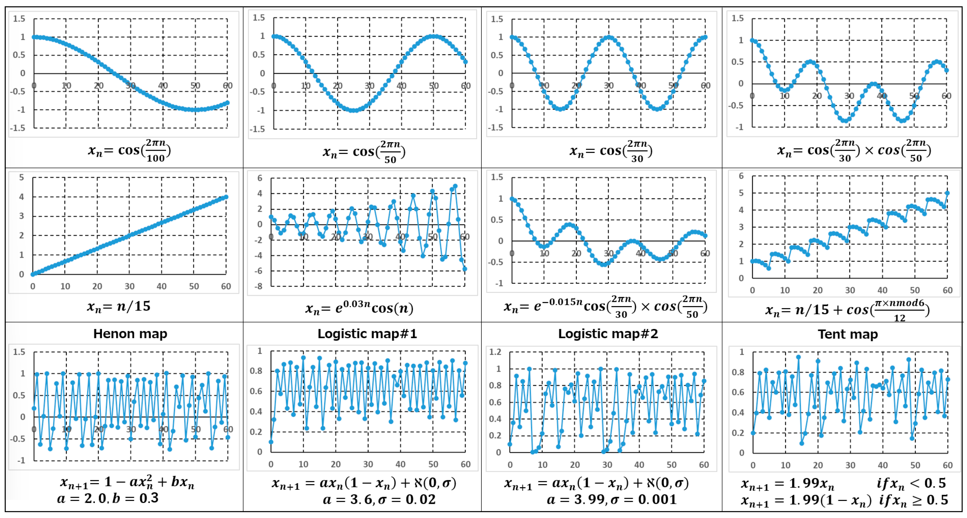
Forecasting trials using test functions were carried out to verify the adequacy of the dynamical forecasting process discussed in Section 2.3 above. The test functions consisted of twelve functions shown in Figure 4. In the figure, the four functions in the top row represent periodicity, the four functions in the middle row indicate trends of increase and decrease, and the four functions in the bottom row show irregularity. The predictability of data containing periodicity and trend variations can be evaluated based on the forecasting results using the function sets from the top and middle rows. On the other hand, the functions in the bottom row, including the Henon map [22], logistic maps [23], and the tent map [24], exhibit chaotic behaviors. The data from logistic maps are also added with a small level of random noise. Therefore, the forecasting capability of data characterized by irregularity and randomness can be assessed using the results of those functions.

The test functions simulate the order history data of service parts, creating time series data corresponding to monthly orders over a period of 61 months. In the forecasting trials, the test data, as shown in Figure 5, sequentially use four months of data obtained by splitting the most recent 12 months of data into three equal segments as the forecast targets, while the prior data is applied as training data.

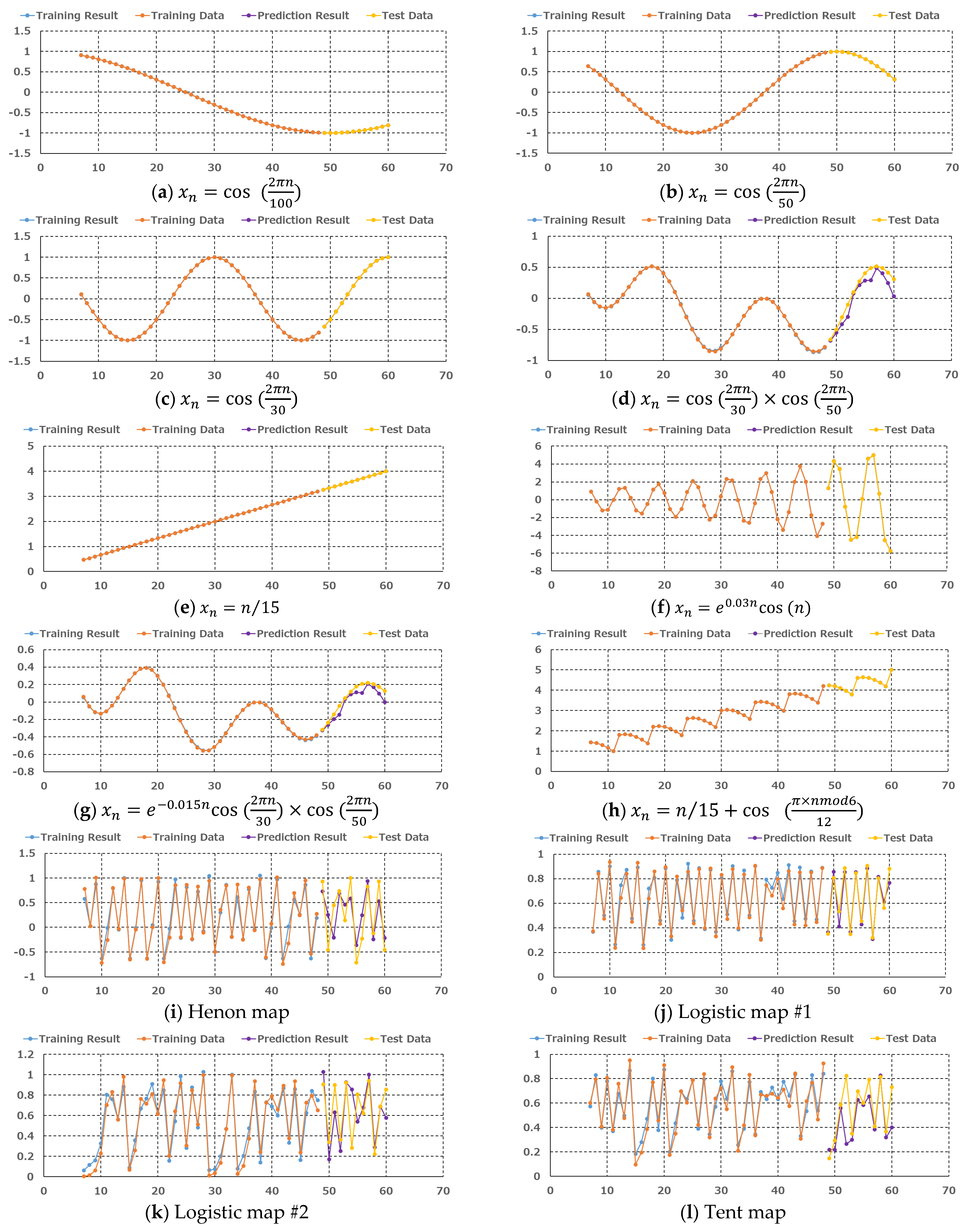
The results of the forecasting trials are presented in Figure 6. In the figure, the time series data of the test functions are divided into the first set of training data used in trial 1 (see Figure 5) and the second set of all test data, along with the corresponding training results and forecasting results. As shown in Figure 6a–h, the training and forecasting results for data with periodicity and trend variations are almost perfectly coincident with the training and forecasting data, indicating very good training and forecasting accuracy. In particular, the forecasting for time series representing trend variations demonstrates high accuracy even outside the range of the training data. This reflects the validity of the dynamical representation for the transition of the regular time series data, and as a result, high accuracy for extrapolated forecasting becomes possible. On the other hand, as shown in Figure 6i–l, while the training and forecasting results for irregular time series data generally reproduce the training and test data, there is a tendency for training and forecasting errors to be larger compared to the results for the regular time series data. One factor contributing to this may be the sensitivity to initial conditions in chaotic systems [25] and the influence of random noise. Therefore, in forecasting time series data that mix regular and irregular variations, better forecasting accuracy can be achieved by separating these two types of variations from the original data.

2.5. Improvement Using EEMD

The results in the previous subsection show some impacts of mode mixing and noise in the numerical calculations of forecasting values. In forecasting a time series pattern that includes both regular and irregular fluctuations, the influence of irregular components may lead to a decrease in overall forecasting accuracy. As a solution to this issue, decomposing complex time series patterns into regular and irregular components using mode decomposition, and then utilizing the mode results for forecasting, will lead to improved forecasting accuracy.

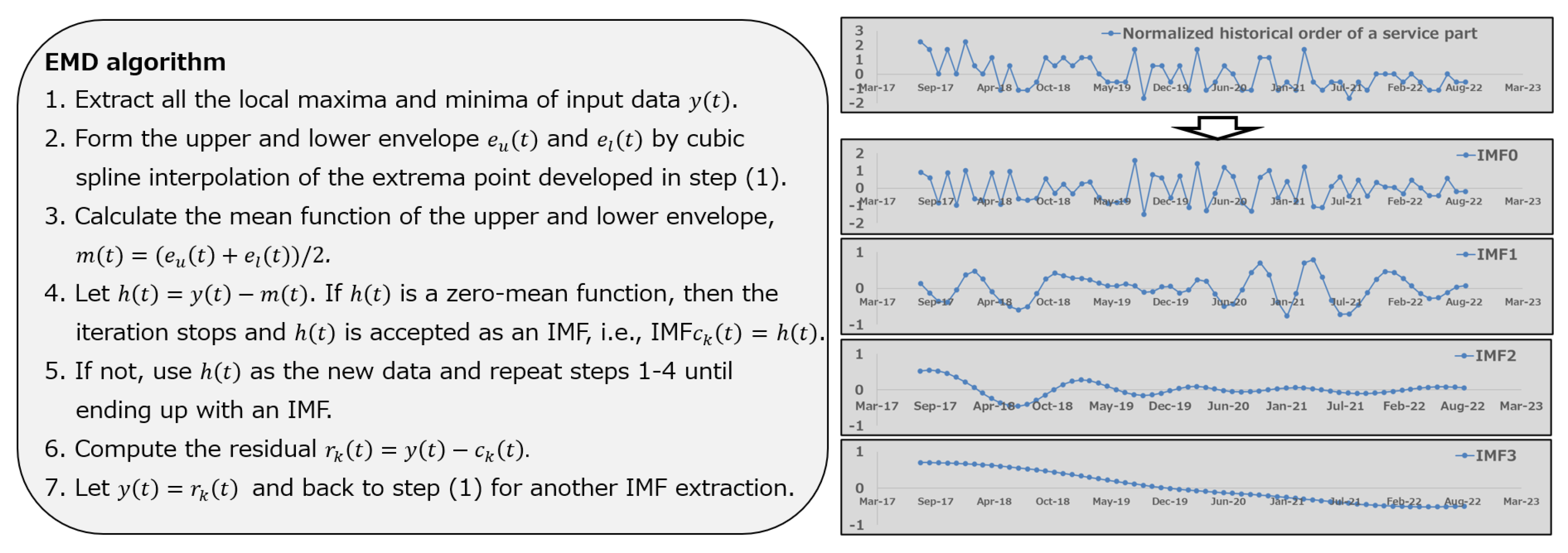
This subsection introduces Ensemble Empirical Mode Decomposition (EEMD) to adaptively decompose any time series into multiple Intrinsic Mode Functions (IMFs) that change at different time scales. EEMD is an improved version of the signal processing algorithm EMD (Empirical Mode Decomposition) proposed by Huang et al. [26]. As shown in Figure 7, the traditional EMD algorithm calculates the upper and lower envelopes of the target signal (time series), determines the average envelope, and then computes the IMF by finding the difference between the average envelope and the target signal, thus decomposing the target signal into multiple intrinsic modes. The characteristic of EMD is that it decomposes the given target signal without assuming basis functions or window functions, allowing for the easy identification of nonlinear oscillation modes at different time scales while preserving the time-frequency characteristics of the target signal. However, since no basis functions are used, the decomposition results may include mixed modes, which presents the challenge of mode mixing [10]. In contrast, the EEMD algorithm, which is an improvement on EMD, adds white noise to the given target signal, then decomposes the signal into various time scales and calculates the decomposition results. This process is repeated multiple times to calculate the ensemble average of the decomposition results, yielding the IMF mode functions. Consequently, EEMD, which enables stable mode decomposition, is considered useful when the data includes complex phenomena such as nonlinearity, non-stationarity, and the presence of noise [27,28,29].

In demand forecasting, EEMD is performed using the historical order data of a single service part as input. An example of EEMD results, shown in Figure 7, reveals that as the order of the IMF increases, the waveform of the IMFs changes from high-frequency fluctuations to low-frequency fluctuations, and eventually to a monotonic increase or decrease. This characteristic allows for a reduction in the complexity of forecasting modeling by decomposing into IMF modes, compared to building a regression model that directly uses order history data. As a result, we can expect enhanced forecasting accuracy for various demand patterns.

Based on the above considerations, we establish a forecasting process that combines Ensemble Empirical Mode Decomposition (EEMD) and Dynamic Mode Decomposition. The process, shown in Figure 8, consists of the following two phases.

• Phase 1: The order history for each service part, i.e., univariate time series, is decomposed into Intrinsic Mode Functions (IMFs) to separate the long-term fluctuation components (regular components) from the short-term fluctuation components (irregular components) included in the data.
• Phase 2: After generating state vectors for each IMF mode, a regression model using Dynamic Mode Decomposition (DMD) based on state vector information as input is trained and used to predict the future values corresponding to each IMF. Finally, the demand forecast is obtained by summing the forecast values for each IMF.

3. Validation Using Historical Order Data of Service Parts

This section introduces a validation methodology for confirming the effectiveness of the proposed method using DMD and EEMD in actual operations. The following subsections detail the dataset, a performance measure, and the two comparative forecasting methods applied in this study.

3.1. Dataset

In inventory management, it is important to guarantee demand forecasting accuracies of service parts that are at risk of stockouts or excess inventory due to demand fluctuations. For this reason, a set of 8,605 service parts was selected based on two criteria: parts that received more than 100 orders in the past three years and parts that experience significant demand fluctuations. The time series data of historical orders for these parts (see Figure 9) were used as validation data. The data period spans from August 2017 to August 2022, with the validation period set from September 2021 to August 2022. Since the lead time for the production and logistics of some service parts is long and future orders may need to be fixed up to four months in advance, the demands four months ahead, including the demand of the current month and the demands of the next three months, were used as the forecasting targets. Therefore, as shown in Figure 5, data in the 12-month validation period was equally divided into three segments, with data from four months in each segment sequentially used as test data and the order history prior to the test data applied as training data. A forecasting model for each forecasting method is trained using training data and is used to forecast the test data in the validation period. The effectiveness of each forecasting method is validated through comparisons of the forecasting results.

3.2. Performance Measure

Instead of using common evaluation metrics such as Mean Absolute Error (MAE) and Mean Absolute Percentage Error (MAPE), this study introduces the score value shown below for error evaluation, with the aim of ensuring the stability of forecasting accuracy over the long term.

$$score={\displaystyle \frac{1}{12}}{\sum }_{t-11}^t\left|e_i\right|,$$

(17)

In Equation (17), the time from $t-11$ to $t$ indicates the validation period corresponding to the current time $t$, and the score is calculated as the average of the absolute values of the errors $e_i$ during this validation period. The error $e_i$ for the validation month $i$ is defined by the following equation.

$$e_i={\displaystyle \frac{({\widehat{\mathit{y}}}_{\mathit{i}}-{\mathit{y}}_{\mathit{i}})}{\frac{1}{12}{\sum }_{i-12}^{i-1}{\mathit{y}}_{\mathit{j}}}}\to \forall i:t-11\le i\le t,$$

(18)

where ${\widehat{y}}_i$ and $y_i$ represent the forecasting value and the actual value for the validation month $i$, respectively. As shown above, the error $e_i$ represents the difference, normalized by the average of the actual data over a year from month $i-12$ to month $i-1$, between the actual order results and the forecasted values. Therefore, it becomes possible to compare forecasting accuracy using the error $e_i$ and score values, even among parts with significantly different demand scales. Furthermore, the use of the score values can avoid the drawback of MAE and MAPE being unable to adequately assess errors with small values. By weighting the denominator in Equation (18), it allows for a balanced evaluation of errors even when the scale of the predicted values varies significantly.

3.3. Comparative Methods

Two forecasting methods are introduced as comparison targets to confirm the effectiveness of the proposed method in practice. Both methods use common techniques from statistical and machine learning approaches for time series forecasting. The outlines of these methods are described as follows.

In the first method, referred to as Comparative Method 1, a combination of simple moving average and exponential smoothing is used to predict the demand values for the next four months (the current month and the next three months). The simple moving average [30] is a calculation of the demand for the current month as the average of the most recent historical order data over a year. In addition, the demands for the next three months are assumed to be equal to the current month’s forecast value. On the other hand, exponential smoothing [31] calculates the demand for the current month as the sum of the previous month’s order data and the previous month’s forecast value, weighted by the smoothing coefficients. Similar to the simple moving average, the demands for the next three months are set to be equal to the current month’s forecast value. In this method, training predictions using both the simple moving average and exponential smoothing are conducted. After evaluating the accuracy of both prediction results, the one with the best performance is selected and used to calculate the future forecast values.

In the second method, referred to as Comparative Method 2, the time series of historical order records for all service parts in the dataset are decomposed into trend components, seasonal components, and residual components using STL decomposition (Seasonal Trend decomposition using Loess) [32]. The trend components extracted through STL decomposition are approximated using polynomial regressions, which can be used to compute the future forecast values for the trend components. On the other hand, the sums of the seasonal components and the residual components are normalized, and the resulting time series are clustered using Ward’s method [33]. The time series, which represents the annual demand pattern, is calculated by averaging the time series within each cluster. The rescaled annual demand pattern is combined with the forecast value of the trend component to produce the forecast value of the global characteristic demand for each individual service part. Subsequently, the residuals, which are the differences between historical order records and the global characteristic demand forecast value for each individual service part, are computed. A regression model, using common machine learning techniques [34,35,36], is trained with the lags in historical order data as input and the residuals as the objective function. Finally, the sum of the predicted values obtained from the residual regression model and the forecast value of global characteristic demand is used as the forecast for future demand for each individual service part. More details of the method can be found in [37].

As mentioned in Section 1, simple moving average and exponential smoothing are two popular forecasting methods used in inventory management. Therefore, Comparative Method 1 represents not only a traditional but also a practical forecasting method. On the other hand, Comparative Method 2 represents an advanced forecasting method in which some state-of-the-art data science techniques are combined. By comparing the proposed method with these two comparative methods, we can confirm not only the effectiveness of the proposed method in practical applications, but also its superiority in the field of forecasting time series data.

4. Results and Discussion

A comparison of score results between the proposed method and two comparative methods is shown in

Table 1. Results of average scores and the number of service parts in score ranges.

	Comparative Method 1	Comparative Method 2	Proposed Method
Average score over 8605 parts	0.370	0.433	0.269
Number of parts with low score (score under 0.3)	4537	4816	6319
Number of parts with intermediate score (score between 0.3 and 0.7)	3373	3129	2051
Number of parts with high score (score above 0.7)	695	660	235

. In the results of average scores, which represent the overall forecasting accuracy of 8,605 parts, the higher score (0.433) of Comparative Method 2 compared to Comparative Method 1 (0.370) highlights the difficulties of ensuring demand forecasting accuracy across a wide range of service parts even when using sophisticated statistical and machine learning techniques for time series forecasting. On the other hand, the forecast produced by the proposed method reduces the average score to 0.269, a decrease of 27% and 38% compared to Comparative Method 1 and Comparative Method 2, respectively. The results indicate that overall forecasting accuracy with high reliability can be achieved by utilizing the proposed method. In the analysis of the relationships between the score values and the number of parts, the number of parts with good forecasting accuracy (those with score values under 0.3) in the proposed method greatly exceeds that of the comparative methods, with a significant increase of about 1500 parts. As a result, the number of parts with intermediate forecasting accuracy (those with score values between 0.3 and 0.7) and low forecasting accuracy (those with score values above 0.7) in the proposed method decreases significantly. However, there is still a small percentage of service parts with low forecasting accuracy in the proposed method, indicating a need to consider improvements in accuracy and management of the forecast values for the demand of these service parts.

Figure 10 illustrates the comparison results of forecasting accuracy advantages in the dataset between the proposed method and each comparative method. The proposed method shows a greater number of advantageous parts compared to the comparative methods, with a ratio of part numbers of 8:1 between the proposed method and Comparative Method 1, and a ratio of part numbers of 7:2 between the proposed method and Comparative Method 2. The results suggest that the use of DMD and EEMD can enhance forecasting accuracy across various demand patterns for different individual parts. Meanwhile, the number of service parts that achieve better forecasting accuracy using the comparative methods implies that there are some demand patterns in which the proposed method is not superior to the others.

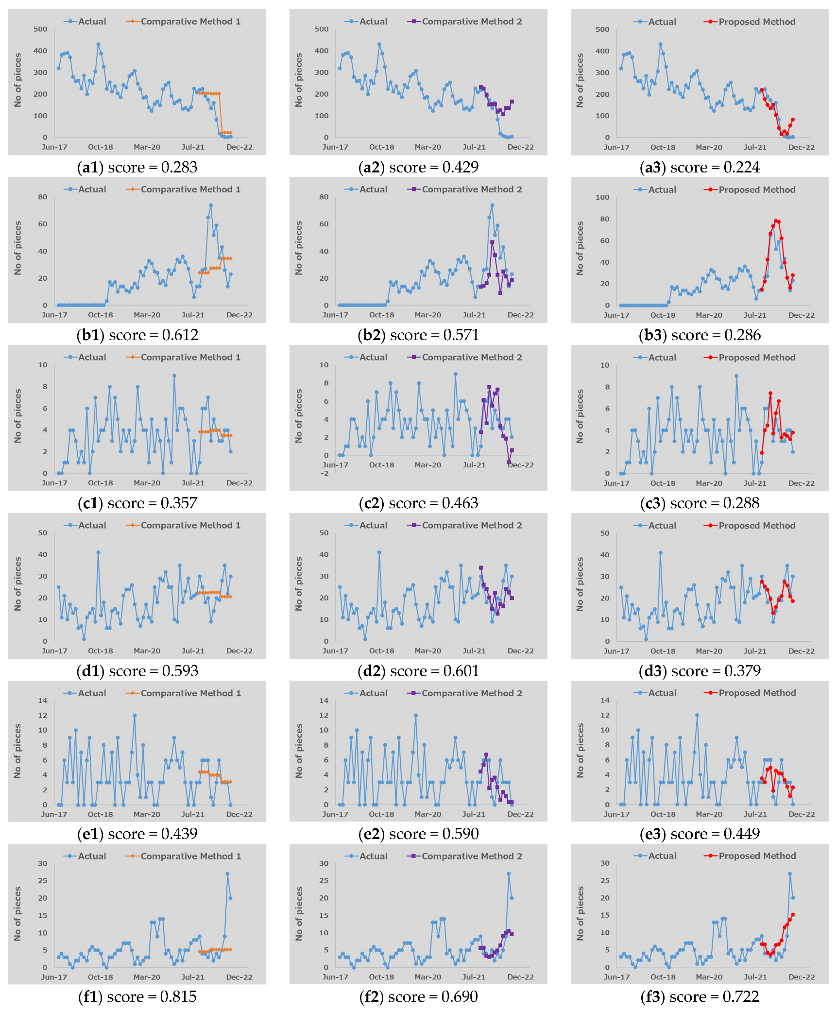
The actual historical orders, forecast waveforms, and the corresponding score values for some representative parts with multiple demand patterns are shown in Figure 11 and Figure 12. In each figure, the results in a row show the forecast results for an individual service part while the left column, the middle column, and the right column show the forecast results using Comparative Method 1, Comparative Method 2, and the proposed method, respectively. First, the results for demand patterns with strong seasonality (annual periodicity) are presented in Figure 11a. The forecast waveforms of Comparative Method 2 and the proposed method demonstrate good accuracy in reproducing annual periodic fluctuations compared to Comparative Method 1, with Comparative Method 2 showing the best results due to its assumption of annual demand patterns in the historical order data of service parts. Conversely, for the demand patterns representing weak annual periodicity (where order quantities fluctuate within a trend of annual periodicity) shown in Figure 11b and the two-year periodic demand pattern shown in Figure 11c, the forecast accuracy of the proposed method exceeds that of Comparative Method 2, suggesting the capabilities of DMD and EEMD for forecasting demand patterns with different periodicities.

Figure 11e,f show the forecasting results in demand patterns dominated by increasing and decreasing trends. In such demand patterns, the proposed method shows slight superiority over the comparative methods even without any assumption of trends. Furthermore, in the demand patterns where the forecast range differs from those in the training range, as shown in Figure 12a,b, the extrapolation forecasts using DMD in the proposed method demonstrate very good accuracy. This result confirms the capability of DMD in extrapolated forecasting not only in test functions but also in real data situations.

In demand patterns with high order quantities and weak variability shown in Figure 11d, all methods yield good accuracy in their forecasting results. On the other hand, in demand patterns characterized by low order quantities and strong variability, the results in Figure 12c,d show the clear superiority of forecasts made by the proposed method. Generally, the proposed method consistently delivers good accuracy across all previously discussed demand patterns, indicating its capability for forecasting both regular and irregular demand patterns where randomness is not a dominant factor.

The qualitative reproducibility of the proposed method in the demand patterns characterized by strong random fluctuations at low order quantity levels is shown in Figure 12e. However, its quantitative forecasting results are still inadequate. In addition, in the demand patterns shown in Figure 12f, where unprecedented demands occur, the current forecasting approaches based on historical order data cannot accurately represent such sudden fluctuations, making reliable forecasting impossible. Therefore, it is necessary to consider improvement measures for the proposed method, which not only predicts future demand but also assesses the range of its possibilities. As a potential solution, we can focus on IMF0, which exhibits the most irregular fluctuations among the modes obtained by EEMD, and consider expressing the time evolution of IMF0 using DMD while taking uncertainty into account. Consequently, the DMD theory that considers probabilities becomes significant, and its development and application can be seen as one of the future prospects of the proposed method.

5. Conclusions

To gain customer satisfaction, manufacturers are required to provide a timely supply of vehicle service parts for accidents and regular consumable replacements. Therefore, while ensuring a safe inventory level to avoid delays in part supply due to stock shortages, excess inventory can lead to an increase in warehouse management costs. For these reasons, demand forecasting of service parts is a critical process for maintaining appropriate inventory levels.

In this paper, a demand forecasting method for vehicle service parts, based on a dynamical approach and time series data, has been developed to satisfy requirements in terms of operation costs and forecasting accuracy. An analytical derivation based on Koopman theory and Dynamic Mode Decomposition (DMD) algorithm, under the assumption that demand transitions can be represented by the dynamics of the corresponding state variables in time series, shows that forecasting for future demands can be achieved by using historical orders of a single service part. Due to this fact, the calculation of the proposed method can be easily applied with reasonable computational requirements.

Forecasting trials using test functions were conducted to theoretically confirm the validity of the proposed method. Excellent agreement between the forecasting values and the test function data shows the capability of the proposed method to predict the future values of various time series data with complex characteristics such as periodicities, trends, nonlinear variability, and chaotic behaviors. Based on trial results, an improvement using Ensemble Empirical Mode Decomposition (EEMD) was implemented to enhance the effectiveness of the proposed method in practice. By applying EEMD, univariate time series data can be decomposed into multiple modes with lower complexity, and as a result, the transition prediction of each mode using DMD can be conducted with higher accuracy.

An application of the proposed method to an order dataset of service parts was also conducted to confirm its effectiveness in practice. A significant reduction in forecasting errors obtained by the proposed method, in comparison with two other forecasting methods, shows its superiority in forecasting various demand patterns of service parts.

Based on all of the above results, the proposed method can be used with high confidence to predict and analyze future demands at the individual service part level. The application of the proposed method is not only for the prediction and evaluation of demands for vehicle service parts but can also be extended to other time series forecasting problems. On the other hand, it was also found that the forecasting accuracy of the proposed method is not satisfactory for unprecedented demand patterns or those that change randomly with low order quantities. In demand patterns dominated by unpredictable factors, achieving safe inventory levels and optimal stock management using current forecasts is still challenging. To overcome this problem, improvements and expansions of the proposed method by applying theories [38,39] that account for uncertainty in time series are required, and this will be addressed in a future work.