Abstract
The effective functioning of an organization is directly related to properly planning the necessary resources. The purpose of the study is to propose a solution for appropriate resource planning to help the decision-maker. An applied approach integrates forecasting using linear autoregressive analysis, optimal determination of regression coefficients as solutions to optimization problems with an embedded least squares method and sliding shift procedure for a new start of historical data. Two linear predictive models were created and validated with real data in a simulation environment under two scenarios. Comparisons were made with the real data, as well as between the two models.
1. Introduction
Energy planning problems are complex problems with multiple decision-makers and multiple criteria. Energy planning determines the optimum combination of energy sources to satisfy a given demand. This is done by taking into consideration the multi-criteria for decision-making, which are quantitative (economic and technical criterion) and qualitative (environmental impact and social criterion) [1]. In [1], an analysis of the development of a multi-level and multi-criteria decision-making structure dedicated to energy planning is presented. A literature review on the various aspects involved in energy planning, focusing on risks, errors, and uncertainties in energy planning, geographical level of energy planning, and validation of planning methods is done in [2].
Regional planning and optimization of renewable energy sources for improved rural electrification is presented in [3] based on the Stackelberg game framework. A bi-level optimization model was used to determine the trade-off between the leader (government) and the follower (the power industry). Sustainable electricity supply planning using a nexus-based optimization approach is studied in [4]. Due to the limited capacity of available energy resources, energy planning with renewable energy sources is proposed in [5]. This work identifies fourteen factors concerning the planning process that would allow for choosing the most appropriate technology for a given city. When planning resources, the question arises about the successful implementation of plans. Plan implementation is a complex process influenced by many factors. In [6], 19 criteria influencing the success of implementation were identified and the impact of these criteria was tested. An implementation evaluation index is constructed to assess the best practices for effective implementation.
In resource planning, an important place is also given to model predictive control (MPC), as it finds wide application in various fields. MPC describes a set of advanced control methods that use a process model to predict the future behavior of the controlled system. A review of MPC including theory, historic evolution, and practical considerations is described in [7]. Model Predictive Control for efficient management of energy resources in smart buildings is discussed in [8].
The application of MPC and its benefits in reactive separation techniques, particularly in the natural gas sweetening process is discussed in [9]. MPC has gained increasing interest in the adaptive management of water resources systems due to its capability of incorporating disturbance forecasts into real-time optimal control problems [10]. Two-scale MPC for resource optimization problems with switched decisions is presented in [11]. The simulation results demonstrate the computational advantages of the proposed algorithm compared to direct problem discretization and optimization. In supply chain planning, it is very important to forecast the changes in the market to maintain an inventory level that is enough to satisfy customer demand. According to the demand uncertainty in the supply chain network, in [12] MPC is applied to solve dynamic optimization of the inventory. A control strategy for biopharmaceutical production by model predictive control was developed in [13]. The development of a decision-making strategy for fulfilling the power and heat demands of small residential neighborhoods is presented in [14]. In [15] a review of progress in the context of motion planning and control for autonomous marine vehicles from the perspective of MPC is provided. A review of model predictive control in precision agriculture is done in [16].
This research aims to create an intelligent tool for planning available resources to assist decision-makers. The aim is to create models that predict electricity consumption in an organization. This will facilitate resource planning in the organization and, through resource reallocation, improve its performance.
2. Forecasting Models
Statistical analysis is a widely applied mathematical apparatus for formalizing the process of predicting data [17,18]. Here we will apply first- and second-order linear regression analysis, through which we will create two forecasting models: AR(1) and AR(2). Subsequently, we will evaluate the accuracy of both models.
We denote the known value at moment t by y(t) and the unknown predicted value at moment t + 1 by yp(t + 1).
The linear autoregressive model AR(1) in the case of m linear equations is of the form
The predicted value at time t + 1 depends on the available value y(t) at time t according to the linear relationship (1), in which the coefficients a and b are unknown and must be determined.
The linear autoregressive model AR(2) in the case of m linear equations is of the form
The predicted value at time t + 1 depends not only on the value at the previous time t, but also on the time before that: t − 1. Here the unknown parameters and must be determined.
The AR(1) model of type (1) and AR(2) model of type (2) can be presented in matrix form
where for the AR(1) model the matrices are
and for the AR(2) model the matrices are
For both models the unknown coefficients a and b for model AR(1) and and for model AR(2) should be determined to provide the best approximation of the linear system of type (1) or (2) respectively. We denote by δ the difference between the actual and predicted value
The best accuracy of the approximation will be when the difference δ has a minimum value. Therefore, we will apply the least squares method to perform the approximation, the formalization of which is in the form of (7) for AR(1) and (8) for AR(2)
The determination of the approximation coefficients using the matrix form of the AR(1) and AR(2) models is done by the least squares method according to (7) and (8) respectively.
The unknown approximation coefficients are determined by differentiating both sides of (9)
Dependence (10) determines the unknown approximation coefficients (or a and b for the AR(1) model and for the model AR(2)). Since these coefficients represent a solution to the optimization problem (7) or (8), minimizing the error ensures maximum approximation accuracy.
3. Model Predictive Control Using Linear Regression Models
Resource planning plays an essential role in the management of an organization. One such expense is the cost of electricity. Future costs depends on consumption and are not known in advance. Therefore, we will forecast next month’s spending using linear autoregressive models. Since we do not contribute to model predictive control, but only use it, no formalization of MPC is applied in the presentation. Here, an approach is proposed for planning electricity costs by integrating model predictive control and the linear regression models AR(1) and AR(2), presented above. These models require data for a past period. In this case, that period is 4 months. Using the two models, the electricity consumption for the next—fifth month is determined, Figure 1a. A shift of the beginning of the period by 1 month is applied, so the prediction is for the next—sixth month, Figure 1b. This procedure is performed sequentially 8 times to predict electricity consumption for the next 8 months. The manager needs to know what the electricity consumption will be for the first month of 2024. As we are using a historical interval of 4 months, this means that the data from months 9 to 12 must be included in the historical interval. However, the AR(2) model needs data for the previous month and the month before that, or we will use the July 2023 data to forecast the consumption in January 2024.
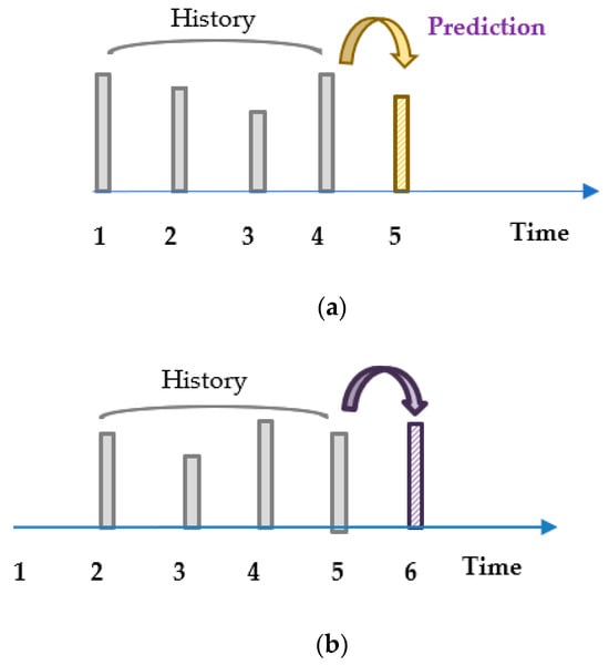
Figure 1.
Model predictive sliding procedure. (a) History start from 1 moment; (b) History start from 2 moment.
The model predictive control is integrated with linear regression analysis that determines the regression models AR(1) and AR(2). Using the least squares method is a prerequisite for minimizing the forecast approximation error because the approximation coefficients are obtained as solutions to an optimization problem (7) or (8). The proposed resource planning approach also includes a sliding forecasting procedure to sequentially move the data used as history.
4. Simulations and Results
4.1. Use Case I: Evaluation of the Two Models Based on Existing Data
Data on electricity consumption in 2023 of a real organization are available, Table 1.

Table 1.
Electricity consumption data for 12 months.
The data from the first 4 months are taken as a historical interval and based on them the consumption value for the 5th month is determined. The predicted value is compared with the real available value and the difference from the approximation is determined according to dependence (6). An optimization problem (7) is solved, the solutions of which determine the approximation coefficients a and b. A shift of 1 month is made.
A system of 4 new equations is compiled with the beginning of the history shifted by 1 month to determine the next forecast value for the 6th month according to the AR(1) model. The same applies to the predictive model AR(2).
For illustration, the calculated optimal values of the coefficients a and b for the AR(1) model are given in Figure 2 and Figure 3, respectively.
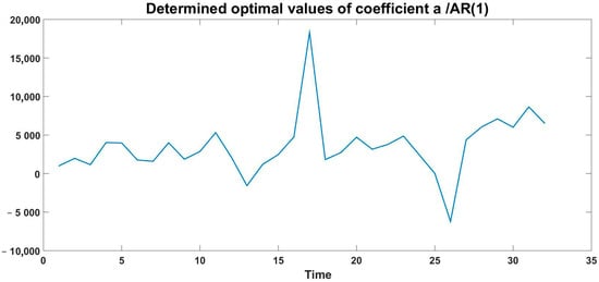
Figure 2.
Calculated optimal values of coefficient a of the model AR(1).
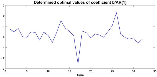
Figure 3.
Calculated optimal values of coefficient b of the model AR(1).
The calculated optimal values of the coefficients a and for the AR(2) model are given in Figure 4, Figure 5 and Figure 6, respectively.
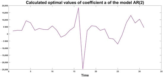
Figure 4.
Calculated optimal values of coefficient a of the model AR(2).
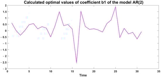
Figure 5.
Calculated optimal values of coefficient of the model AR(2).
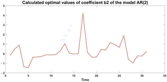
Figure 6.
Calculated optimal values of coefficient of the model AR(2).
Table 2 gives the values of the predictions for 2023 according to the two models, as well as the approximation errors δ. The actual and predicted values according to the AR(1) model, as well as their average values, are presented in Figure 7. The accuracy of the approximation is very good, which also follows from the minimal difference in the average values.
Table 2.
Current and predicted values.
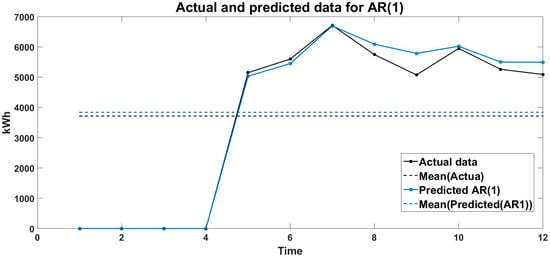
Figure 7.
Actual and predicted data from model AR(1).
The differences between actual and predicted values are presented graphically in Figure 8.
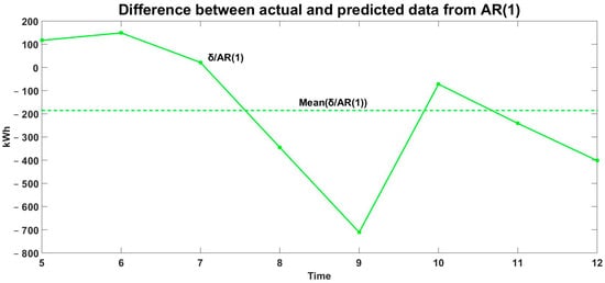
Figure 8.
Difference between actual and predicted values from model AR(1).
Figure 9 presents the actual and predicted values according to the AR(2) model. The predicted values here are from the sixth to the 12th month, with the predicted values coinciding with the actual values.
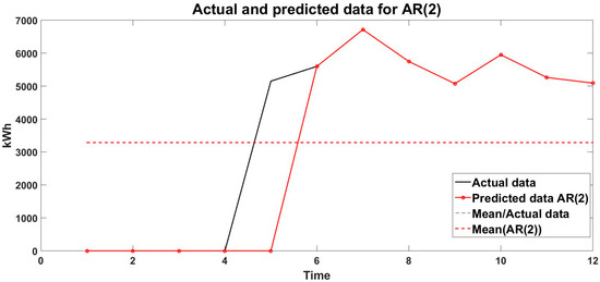
Figure 9.
Actual and predicted data from model AR(2).
The differences between actual and predicted values δ with the AR(2) model are presented in Figure 10.
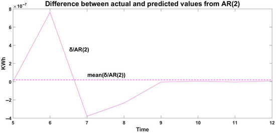
Figure 10.
Difference between actual and predicted values from AR(2).
The average error values from the approximations with the two models are presented in Figure 11.
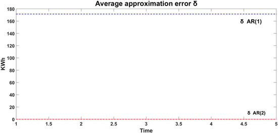
Figure 11.
Comparison between mean approximation error δ of AR(1) and AR(2).
The average value of the approximation for AR(1) is 171 kWh, while for AR(2) it is 0. The better accuracy of the approximation for the second model is due to the fact that in addition to the data from the previous month (as in the first model), the model also includes data from another month ago.
4.2. Use Case II: Model Predictive Control with Insufficient Data for Approximation
Usually, at the end of the year, company managers have to plan their expenses for the next year. In our case, with the available data on electricity consumption for 2023, it is necessary to forecast the consumption for 2024. The forecasting approach here has been changed, since at the end of 2023 there are no data available on electricity consumption in 2024. To optimally determine the approximation coefficients as solutions to the optimization problems (7) and (8), we will use the predicted values as real data.
The required historical data for the linear regression analysis are the data from the last 4 months of 2023. In addition, for the AR(1) model, we need to take the data from the previous month (August), and for the AR(2) model one month back (July). In other words, to make forecasts using both models, 6 months of data are needed. Thus, the required data for forecasting consumption in January 2024 starts from July 2023 according to Table 3.
Table 3.
Data required for forecasting 2024.
The available data from July to December 2023 are used as a history in order to predict the electricity consumption in January 2024. We use the forecasting approach described above and determine the forecasting value for January 2024 for both models, Table 4.
Table 4.
Actual and predicted values for January 2024.
To make a forecast for February 2024, we need the data for the previous 6 months. According to the proposed approach, the beginning of the history is shifted by 1 month (starting from August) and the forecast value from January 2024 is also included as history, Table 5.
Table 5.
Actual and predicted values for February 2024.
Similarly, forecasts are made for the following months for 2024. Starting from 12/23, a forecast is made for June/24. This exhausts the available data from 2023 and further on, the forecasted data are used as history. Table 6 presents the data for the last forecast made for August 2024.
Table 6.
Predicted values for August 2024.
The same procedure can be applied to forecast values for the coming months, but we limit ourselves here.
It is interesting to evaluate the forecast using this approach. Therefore, after the availability of data on actual consumption in 2024, a comparison between actual and forecasted values was made. The data are presented in Table 7, and the graphical representation can be seen in Figure 12.
Table 7.
Actual and predicted values for 2024.
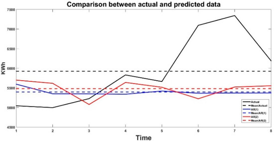
Figure 12.
Comparison between actual and predicted data for 2024.
The figure shows that the predicted values for June and July are significantly lower than the actual values. The variation of the approximation error for the two models is given in Figure 13.
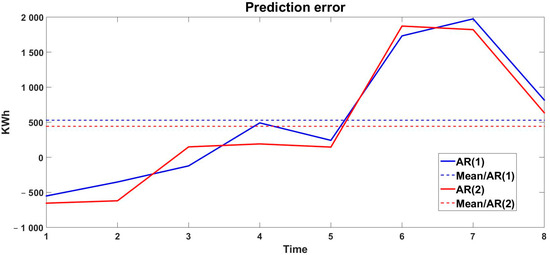
Figure 13.
Variation of approximation error.
From the average error value it follows that the accuracy of the AR(2) model is better than that of AR(1). The mean error of model AR(1) is 530 kWh and the mean error of AR(2) is 442 kWh.
5. Conclusions
The study presents an approach to resource planning using model predictive control. The contribution of the study is creating a tool that supports decision-making by integrating several technologies for better resource planning. Two predictive linear autoregressive models have been developed. In order to achieve greater accuracy in linear approximation, the linear coefficients have been determined in an optimal way as solutions to optimization problems to minimize forecasting errors. In model predictive management, a procedure of sequential displacement of historical data has been applied.
The model evaluations were performed in two ways in a numerical simulation environment. Real data on the electricity consumption of an organization for 12 months for 2023 were used. In the first case, forecasts were made within the year according to both models. Comparisons were made between the real and forecasted values for both models. The results of the numerical modeling give an advantage to the forecasting of the second model—AR(2) in terms of accuracy.
The second way of evaluating the models was carried out by sequentially forecasting the electricity consumption values for 2024 using the necessary historical data from 2023. The peculiarity here is that instead of real data, the forecasted data for 2024 are used. In this way, forecasts were made for 8 months for 2024. Subsequently, the two models were evaluated with the obtained real data for 2024, with again higher accuracy being achieved with the AR(2) model.
The results obtained provide grounds for applying the proposed approach in various areas to assist in decision-making in the management of organizations.
In further research, more complex models such as ARIMA, MAPE etc. will be applied to achieve a better approximation and to make a comparison on a broader basis.
Author Contributions
Conceptualization—T.S.; Methodology, K.S. and T.S.; software, K.S.; formal analysis, K.S. and T.S.; writing—original draft preparation, K.S.; writing—review and editing, T.S. and K.S.; supervision, G.A.; project administration, G.A. All authors have read and agreed to the published version of the manuscript.
Funding
This research was funded by NEXT GENERATION PROGRAM, grant number BG-RRP-2.017-0031-C01, “Research and development of a smart Energy system for eco-charging of electric vehicles, using reNEWable energy sources—RENEW” and from the EU’s Horizon Eu-rope Widening programme via COALition project “Promoting Innovation Excellence in Transfor-mation of Coal Regions to Climate-Neutral, Thriving Economies”, grant agreement No 101087022.
Institutional Review Board Statement
Not applicable.
Informed Consent Statement
Not applicable.
Data Availability Statement
Data is contained within the article.
Conflicts of Interest
The authors declare no conflicts of interest.
Abbreviations
The following abbreviations are used in this manuscript:
| MPC | Model Predictive Control |
| AR(1) | Auto-regressive model with one previous value from the time series |
| AR(2) | Auto-regressive model with two previous values from the time series |
References
- Thery, R.; Zarate, P. Energy planning: A multi-level and multicriteria decision-making structure proposal. Cent. Eur. J. Oper. Res. 2009, 17, 265–274. [Google Scholar] [CrossRef]
- Prasad, R.D.; Bansal, R.; Raturi, A. Multi-faceted energy planning: A review. Renew. Sustain. Energy Rev. 2014, 38, 686–699. [Google Scholar] [CrossRef]
- Shahrom, S.F.; Aviso, K.B.; Tan, R.R.; Saleem, N.N.; Ng, D.K.S.; Andiappan, V. Regional Planning and Optimization of Renewable Energy Sources for Improved Rural Electrification. Process Integr. Optim. Sustain. 2023, 7, 785–804. [Google Scholar] [CrossRef]
- Jafar, H.T.; Tavakoli, O.; Bidhendi, G.N.; Alizadeh, M. Sustainable electricity supply planning: A nexus-based optimization approach. Renew. Sustain. Energy Rev. 2024, 195, 114316. [Google Scholar] [CrossRef]
- Narváez, F.A.S.; Castro, E.I.M. Energy planning with renewable energy sources. Int. J. Phys. Sci. Eng. 2021, 5, 44–51. [Google Scholar] [CrossRef]
- Joseph, C.; Gunton, T.I.; Day, J.C. Implementation of resource management plans: Identifying keys to success. J. Environ. Manag. 2008, 88, 594–606. [Google Scholar] [CrossRef] [PubMed]
- Schwenzer, M.; Ay, M.; Bergs, T.; Abel, D. Review on model predictive control: An engineering perspective. Int. J. Adv. Manuf. Technol. 2021, 117, 1327–1349. [Google Scholar] [CrossRef]
- Simmini, F.; Caldognetto, T.; Bruschetta, M.; Mion, E.; Carli, R. Model Predictive Control for Efficient Management of Energy Resources in Smart Buildings. Energies 2021, 14, 5592. [Google Scholar] [CrossRef]
- Karthigaiselvan, K.; Panda, R.C. Implementation of MPC Strategy in Reactive Separation Techniques and Its Benefits: A Demonstration with Natural Gas Sweetening Process. In Model Predictive Control—Theory and Applications; Volosencu, C., Ed.; SDG Publishers Compact: London, UK, 2023. [Google Scholar] [CrossRef]
- Castelletti, A.; Ficchì, A.; Cominola, A.; Segovia, P.; Giuliani, M.; Wu, W.; Lucia, S.; Ocampo-Martinez, C.; Schutter, B.D.; Maestre, J.M. Model Predictive Control of water resources systems: A review and research agenda. Annu. Rev. Control 2023, 55, 442–465. [Google Scholar] [CrossRef]
- Balaguer-Herrero, P.; Alfonso-Gil, J.C.; Martinez-Marquez, C.I.; Navarro, G.M.; Orts-Grau, S.; Segui-Chilet, S. Two-Scale Model Predictive Control for Resource Optimization Problems With Switched Decisions. IEEE Access 2022, 10, 57824–57834. [Google Scholar] [CrossRef]
- Hai, D.; Hao, Z.; Ping, L.Y. Model Predictive Control for inventory Management in Supply Chain Planning. Procedia Eng. 2011, 15, 1154–1159. [Google Scholar] [CrossRef][Green Version]
- Eslami, T.; Jungbauer, A. Control strategy for biopharmaceutical production by model predictive control. Biotechnol. Prog. 2024, 40, e3426. [Google Scholar] [CrossRef] [PubMed]
- Mechleri, E.; Dorneanu, B.; Arellano-Garcia, H. A Model Predictive Control-Based Decision-Making Strategy for Residential Microgrids. Engineering 2022, 3, 100–115. [Google Scholar] [CrossRef]
- Wei, H.; Shi, Y. MPC-based motion planning and control enables smarter and safer autonomous marine vehicles: Perspectives and a tutorial survey. IEEE/CAA J. Autom. Sin. 2023, 10, 8–24. [Google Scholar] [CrossRef]
- Bwambalea, E.; Wanyamaa, J.; Adongo, T.A.; Umukiza, E.; Ntole, R.; Chikavumbwa, S.R.; Sibale, D.; Jeremaih, Z. A review of model predictive control in precision agriculture. Smart Agric. Technol. 2025, 10, 100716. [Google Scholar] [CrossRef]
- Zohuri, B.; Mossavar-Rahmani, F.; Behgounita, F. Chapter 21—Statistical forecasting—Regression and time series analyses. In Knowledge Is Power in Four Dimensions: Models to Forecast Future Paradigm; Zohuri, B., Mossavar-Rahmani, F., Behgounia, F., Eds.; Elsevier: Amsterdam, The Netherlands, 2022; pp. 709–722. [Google Scholar]
- Kamran, M. Chaper 8—Energy statistics and forecasting for smart grids. In Fundamentals of Smart Grid Systems; Elsevier: Amsterdam, The Netherlands, 2023; pp. 365–392. [Google Scholar] [CrossRef]


Disclaimer/Publisher’s Note: The statements, opinions and data contained in all publications are solely those of the individual author(s) and contributor(s) and not of MDPI and/or the editor(s). MDPI and/or the editor(s) disclaim responsibility for any injury to people or property resulting from any ideas, methods, instructions or products referred to in the content. |
© 2025 by the authors. Licensee MDPI, Basel, Switzerland. This article is an open access article distributed under the terms and conditions of the Creative Commons Attribution (CC BY) license (https://creativecommons.org/licenses/by/4.0/).