Proceeding Paper

Acoustic Positioning System for 3D Localization of Sound Sources Based on the Time of Arrival of a Signal for a Low-Cost System †

by
Dídac D.Tortosa
1,*,‡,
Iván Herrero-Durá
2,‡ and
Jorge E. Otero
3,‡
1
Institut d’Investigació per a la Gestió Integrada de Zones Costaneres (IGIC), Universitat Politècnica de València (UPV), Carrer del Paranimf 1, 46730 Gandia, Spain
2
KFB Acoustics Sp. z o. o. Mydlana 7, 51-502 Wrocław, Poland
3
Instituto Tecnoacústico de Cantabria (ITC), Calle Vargas 55, 39010 Santander, Spain
*
Author to whom correspondence should be addressed.
Presented at the 8th International Electronic Conference on Sensors and Applications, 1–15 November 2021; Available online: https://ecsa-8.sciforum.net.
These authors contributed equally to this work.
Eng. Proc. 2021, 10(1), 15; https://doi.org/10.3390/ecsa-8-11307
Published: 1 November 2021

Abstract

:
The localization of sound sources has received increasing interest over the last few decades, given its wide range of applications. The triangulation method using the Time of Arrival (ToA) of a signal has shown to be useful and easy-to-use and, at the same time, provides accurate results. In this work, the acoustic trilateration method is applied in experimental measures to study and demonstrate its precision in air. Firstly, the method is tested in an anechoic chamber (low reverberating environment) demonstrating its functionality and accuracy. The next step has been the application of the method by using a low-cost system to demonstrate how a non-anechoic environment affects the accuracy of the localization. The detection of the received signal is implemented using a cross-correlation method in the time domain for both cases. Furthermore, the influence of the number and positions of the receiver that are used for this process in the accuracy of the results is also studied.

1. Introduction

Sound localization can be defined as the process of identifying the spatial coordinates of a sound source (emitter) based on the sound signal received by an array of microphones (receivers) [1]. The localization of sound sources by means of arrays of sensors has been one of the central problems in radar, sonar, navigation, geophysics and acoustic tracking [2]. The localization of a source in space has also received an increasing interest over the last years, as many new applications can obtain substantial benefits from the knowledge of the spatial position of an emitter by means of knowing the characteristics of the signal [1].
One the one hand, the identification and characterization of sound sources affecting the environment has a significant importance, as it can contribute to the planning and mitigation of unwanted noise sources, among which it is possible to include road traffic [3,4,5], railway traffic [6,7], noise at airports [8,9], port activities [10,11] and wind turbines [12,13,14]. Otherwise, there is a wide variety of fields in which audio processing applications can be used for source localization, such as animal detection in the wild forest, speech enhancement, tracking of sound sources, maritime applications, localization of brain tumors, teleconferencing, and detection of astroparticles, among others. In this context, the development of new technologies allows a higher accuracy in the process related to the time parameters associated to the localization process [15].
The localization of a source using as a starting point acoustic information is a complex task. The process is composed of different steps, whose accuracy will contribute to the error and resolution in the final detection. In the process of locating a point source, the first step is to identify the signal that is emitted by it and to record that signal in, at least, three different positions in space. These positions must be known with as much accuracy as possible in order to reduce the error in the localization algorithm. Once the signal has been recorded, the next step is the identification of the emitted signal that has been detected by the receivers (detection analysis). This step may require the application of different filtering and processing techniques of the signal, depending on the background noise, the power level of the received signal, and the response of the receiver in the frequency range of interest. The detection step consists of find the recorded signal and assigning a Time of Arrival, ToA, defined as the time that an emitted signal take to be detected by a receiver. Some acoustic detection techniques are based on the use of cross-correlation [16], special thresholds [17] or spectrograms working in the frequency domain [18]. Once the starting point of the signal in the recording is known, it can be studied in more detail, e.g., by estimating the received level or the signal duration.
In the case of a passive acoustic system, in which the source is not controlled by the acquisition system itself (a so-called asynchronous transmitter-receiver system), the detection process can be even more complex. Some examples of these systems can be found in environmental acoustics applications, in which only the receiving elements are controlled, e.g., in road traffic studies [3,4,5], noise at airports [8,9], or port activities [10,11]. Additionally, the number of sources to be located can be unknown in many cases, which makes the detection process of a specific source more complex. Nevertheless, this work is focused on the use of an active acoustic system which centrally and synchronously controls both the transmitter and the receiver, ensuring the capture of the signal emitted by the source at the receivers [19]. This assumption facilitates the localization process and ensures that the efforts are focused on the localization algorithm, instead on the detection algorithm.
Many algorithms and techniques related to the localization process commonly involve an estimation of Time Difference of Arrival, TDoA, of the signal at a set of microphones’ positions. Using these data as a starting point, information about the spatial position of the source can be obtained [20]. The processing of this information is usually based on the computation of the Generalized Cross-Correlation, GCC, whereby the Time of Arrival, ToA, can be obtained [21]. The inverse process can also be used for the localization of a receiver by knowing the localization of different emitters [22].
In this work, the localization of an acoustic source based only on the ToA information by means of the cross-correlation technique is developed. In these type of systems, the distance between the emitter-receiver can be obtained from the information of the ToA in the localization algorithm. The choice of this method is based on its low computational cost and the possibility to use it in semi real-time applications using low-cost systems. The method is initially applied to a system located in an anechoic chamber with the goal of studying its accuracy in a controlled environment and design the optimal configuration of the emission-detection-positioning process. Once the method has been tested in these conditions, it is applied in a low-reverberating environment by using low-cost commercial equipment.
The structure of this paper is as follows: Section 2 presents the case of study and describes the methodology used for the definition of the emitted signal, its detection in recorded signals and the localization of the emitter. In Section 3, the set-up used during the experimental measurements, as well as the results obtained by means of these measurements, are exhibited. Finally, the conclusions and important remarks of this work are presented in Section 4.

2. Methodology

The first step in the study is defining the signal that is used to localize the sound source. Once this signal is emitted by the source (emitter), it propagates through the medium and reaches the receivers. The propagation medium considered in this work is air. It is important to note that, assuming an homogeneous medium in which the speed propagation of the sound waves, c, is constant, the signal takes a different time to reach each receiver placed at a different position due to the different distances to be travelled by the sound waves.
The Time of Flight, ToF, of the signal is a crucial parameter involved in localizing the source, as it represents the time that the signal takes to travel from the emitter to the receivers. The Time of Emission, ToE, is defined as the time instant in which the signal starts being emitted. This parameter can be independent of the data acquisition system, in which case it must be considered as an unknown (passive acoustic system). Finally, the Time of Arrival, ToA, is referred to as the time that the signal takes to be detected by the receiver. From these two last parameters (ToE and ToA), one can straightforward obtain the ToF as
T o F = T o A T o E .
The distance between the emitter and the receiver, d E R , can be defined as a function of the ToF and the speed of sound as
d E R = T o F · c .
The ToE is controlled in the experimental work (see Section 3) by the signal acquisition system and, consequently, the ToA for each receiver is the unknown parameter that must be found.
In this work, the localization of an emitter, E, whose position is theoretically unknown is carried out by means of the signal detected by a receiver, R, placed at different positions. Since a single receiver is used, it is moved to different measurement positions in order to simulate an array of receivers.
Different signals were tested in the experimental stage in order to study which of them allows a more accurate detection of the emitter. After the test, and based on previos studies, Ref. [16] it was found that sweep and MLS are more suitable for the GCC detection.
The linear sine sweep signal, W s , is defined as
W s t = sin 2 π f 2 f 1 T · t + f 1 t ,
where T is the duration of the signal, f 1 the initial frequency of the sweep, f 2 the ending frequency of the sweep and t the instant of the time. Note that if the value of f 1 is lower than that of f 2 , the resulting sweep signal is ascendant (in the opposite case, it is a descendant sine sweep).
For the low-cost system in the case of a reverberating environment, the sine sweep is generated in the frequency range between 2 kHz and 12 kHz and with a duration of 300 ms, both characteristics corresponding to audible signals. A sampling frequency of 44.1 kHz is considered. Details on the emitted, received and correlation signal can be observed in Figure 1.
In order to validate the detection of the signal, a simple virtual measurement is created with the following characteristics: The distance between emitter and receiver, d E R , is 43 cm, and the propagation speed of sound in the surrounding medium is considered as c = 343.2 m/s (with a room temperature of 20 C). With this information one can directly obtain the ToF of the signal as T o F = d E R / c . As it can be observed in Figure 1c, a ToE of 400 ms is considered, resulting in a ToA of 401.2573 ms. The Signal-to-Noise Ratio (SNR) in reception of the signal of 40 dB and a recording time is 1 s are considered (see Figure 1c,d).
It is important to note that, for the sake of simplicity, in the case presented here the decay of the amplitude of the propagating signal with the distance, as well as the variation of the absorption due to the propagation of the sound waves in the medium depending on the frequency, are not considered.

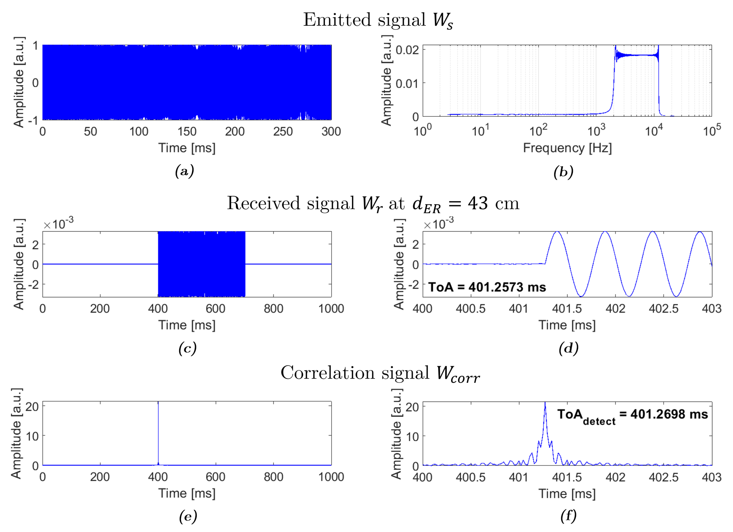
2.1. Detection of the Signal

In this Section, the detection process of the emitted signal is presented. It is important to consider beforehand that a high resolution in the ToA is crucial for an accurate localization process. Since the emitted signal is a sweep, the GCC is an effective method for its automatic detection. This method is based on the correlation of the emitted and received signals and finding the ToA from the peak in the received signal in a given instant of time. The results of this process are shown in Figure 1e,f. As it can be extracted from the difference between the detected ToA from the correlated signal ( T o A d e t e c t , in Figure 1f) and that of the received signal (Figure 1d), there is a delay of 12.5 μ s. Considering the propagation speed of sound in the medium, this delay implies a time difference of less than 0.5 cm in the detection of the signal, which can be assumed as sufficiently low.
Alternative methods can be used with the purpose of finding the ToA, such as using a threshold in the time domain for the amplitude of the received signal or applying the accumulated frequency of the received signal and detecting harsh changes in the slope [23].
The cross-correlation signal, W c o r r , obtained by computing the GCC between the emitted signal, W s , and the received signal, W r , is expressed as a function of the power spectral density G W s W r as follows:
W c o r r G C C ( t ) = + W s ( f ) W r * ( f ) G W s W r ( f ) e i 2 π f t df = φ G C C ( f ) G W s W r ( f ) e i 2 π f t df ,
where the superscript * indicates the complex conjugated value and φ G C C ( f ) is a frequency-dependent weight function. Due to finite observations, it is only possible to obtain an estimation of G W s W r ( f ) [24]. Therefore, to obtain the TDoA, the following expression will be used [25]:
W ^ c o r r G C C 1 ( t ) = + φ G C C ( f ) G ^ W s W r ( f ) e i 2 π f t df ,
where G ^ W s W r ( f ) is the obtained estimation of G W s W r ( f ) . For each pair of sensors, the ToA is taken as the time delay that maximizes the cross-correlation between the filtered signals of both sensors, that is: τ ^ i j G C C = arg max t { W ^ c o r r G C C 1 ( t ) } .

2.2. Localization of the Emitter

A general model for the three-dimensional (3-D) estimation of the position of an emitter using i receivers is developed in this Section. To obtain the location of the sound source, the first step is to know the spatial position ( x i , y i , z i ) in a Cartesian coordinate system of a given number of receivers. Let the position of the emitter to be located be ( x E , y E , and z E ), the distance between the emitter and the i-th receiver, d E R i , is defined as:
d E R i = ( x i x E ) 2 + ( y i y E ) 2 + ( z i z E ) 2 .
Based on Equation (6), it is possible to create a solvable nonlinear equation system with 3 unknowns ( x E , y E and z E ) and i equations. Thus, it is necessary to have a minimum of 3 receivers to solve the system. The system of equations is solved in this method by means of the analysis of the difference in the distance between the i-th receiver and the first receiver ( d i 1 ), which is given by:
d E R i 1 = d E R i d E R 1 = = ( x i x E ) 2 + ( y i y E ) 2 + ( z i z E ) 2 ( x 1 x E ) 2 + ( y 1 y E ) 2 + ( z 1 z E ) 2 ,
where d E R i 1 is the distance between the first receiver and the emitter.
To obtain the position of the source, the system of equations can be written considering a system of m equations and n unknowns f m ( x 1 , x 2 , x 3 , , x n ) = 0 . This system can be written in vector form as f ( x ) = 0 , where f is a vector of m dimensions and x is a vector of n dimensions. To solve this system of equations, it is necessary find a vector x such the function f ( x ) equals the null vector. In this work, the problem is solved by means of an algorithm, based on the MATLAB tool f s o l v e , able to solve nonlinear equations systems. This method is based on the Newton-Raphson method for which an initial position of reference, Pos ref, is proposed to start the calculation process. Since the positions of the receiving microphones are known for all the experimental measurements, the mean value of the receivers’ positions (in the middle between them) has been taken as the reference position. To ensure the convergence of the results, the input parameters of the function have been defined considering a maximum of 4000 iterations, a computational error for the tolerance defined as 10 3 m, I n f maximum function evaluations and not using a Jacobian solution.

3. Experimental Framework and Results

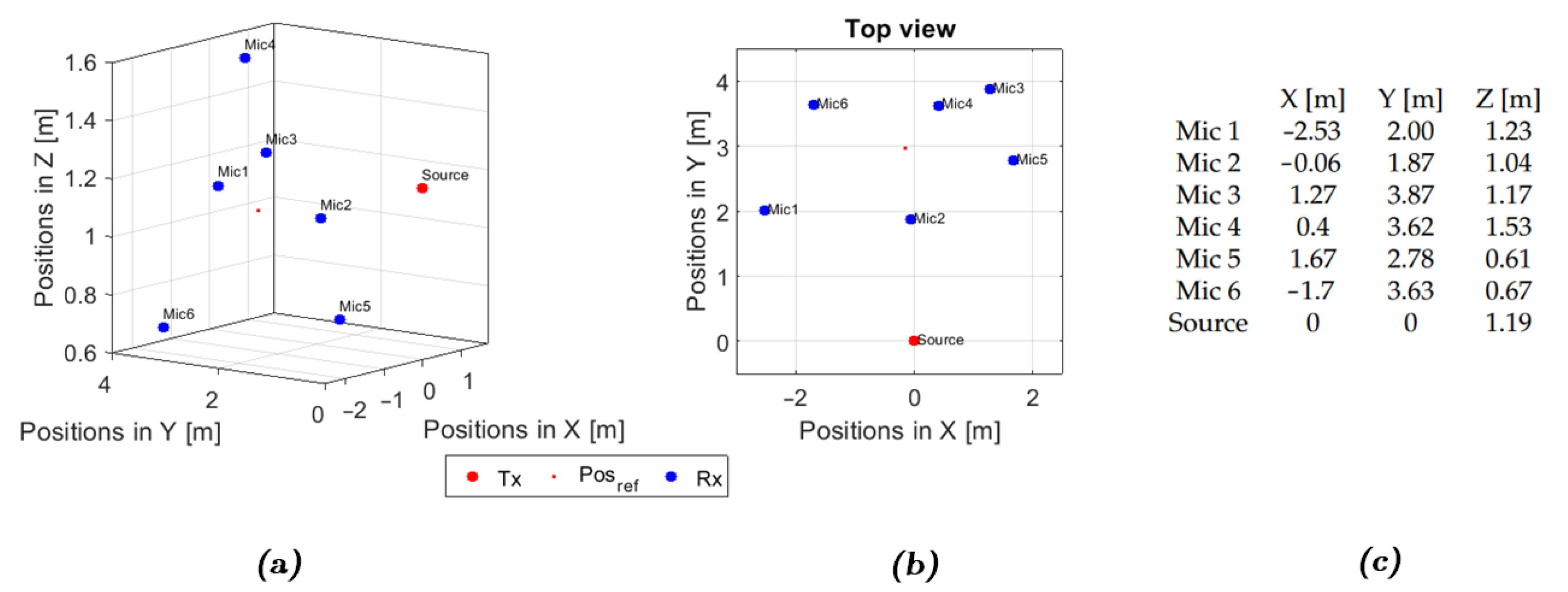
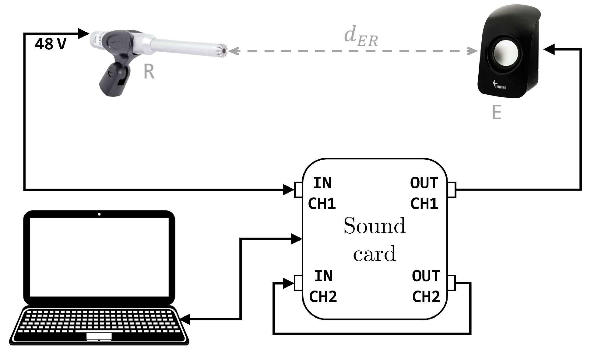
3.1. Experimental Set-Up

In the previous Section, the theoretical approach for the localization of a sound source by solving a system of nonlinear equations has been detailed. This method is used to localize a sound source in two different environments: An anechoic chamber and a low reverberating room. This approach in based on the case in which a given emitter, whose position is unknown, wants to be localized by means of the signal received in certain known locations. The influence of the number of positions for the receiver in the resulting localization is also studied by comparing the results obtained with a different number of considered positions (modifying the number of microphones used in the measurements).
A sound source (emitter), controlled by a sound acquisition system and placed at a given position, emits a signal containing the frequencies within the range of study. This signal is generated by the sound card and registered by a receiver placed at different known positions. In order to obtain reliable results, it is important to make sure that both, emitter and receiver, have a flat frequency response in the studied bandwidth.
(a)
Measurements in an anechoic chamber
In order to validate the acoustic positioning system for 3D localization, previously described for a low-cost system, the same method in an ideal anechoic conditions has been applied. The approach consists of testing different signals and study the results to select the best configuration to be reproduced afterwards with the low-cost system. In this occasion, a Focusrite Scarlett 18i20 v3 audio card (Focusrite, Buckinghamshire, England) was used, connected to 6 microphones Behringer ECM8000 (Behringer, Willich, Germany) (array distributed among 3.2 and 4.1 m distance from the emitter) and to a Genelec 8030A (Genelec, Iisalmi, Finland) source. This source is composed of a woofer speaker for low and mid frequencies (below 2 kHz) and a tweeter for high frequencies (above 2 kHz). In the case that the emitted signal contains only high frequency components the emitter, E, to be searched is the center of the tweeter position. If, on the contrary, the signal includes all the audible spectrum (e.g., MLS) the E position to be found corresponds to the center position between the tweeter and the woofer.
In order to calibrate the detection and localization algorithms, it is necessary to test them in different controlled environments. A simulated environment, in which simulations with a different number of sensor points (3, 4, 5 and 6) have been carried out for different combinations of sensors and theoretical sources, has been defined. Figure 2 shows a representation of the positions of the receivers together with one of the source points for which their spatial coordinates are known.
With this, it is possible to create a controlled simulated environment. Thus, to test the results of the localization of a source reconstructed by the localization algorithm, an error value with respect to the real values of its position was randomly added and 1000 simulations were performed in each case.
Figure 3 shows an overview of the results provided by the localization algorithm. In all the cases, the abscissa axis shows the difference between the reconstructed position and the real position of the source while the ordinate axis shows the error added to the real position.
On the one hand, as expected, for a larger number of sensors the reconstruction of the source considerably improves. On the other hand, when the error increases, the reconstruction of the source is more affected in a combination of 3 sensors, while for combinations of 4 or more sensors the results are independent of the error. This indicates that for combinations of at least 4 sensors it is sufficient to obtain results with good precision and higher robustness.
After testing the results of the location algorithms, it is necessary to test the detection algorithms. In this sense, We have generated different signals type (sine, MLS and sweep) by using an electro-mechanical loudspeaker with a 4-inch cone inside an anechoic chamber.
For this case, to determine the precision in the detection algorithms, it has been decided to add an error in the distances of the detected signals. Thus, Figure 3 shows the results where the abscissa axis indicates the number of microphones used and the ordinate axis indicates the added error.
Thus, in terms of error, the results improve when a set of 4 sensors is used. Although the results of the source reconstruction using only the location algorithm are reliable, by implementing signal detection algorithms for the TDOA value, the source reconstruction worsens. This can be due to errors caused by correlation detection between the signals, by a low sampling in the capture devices or by small temporal differences due to the mechanical components produced in the loudspeaker and in the microphones.
Additionally, four signal types were tested in the anechoic experimental set-up using 3, 4, 5, and 6 microphones: MLS, sweep (10 Hz to 22 kHz), sinus of 500 Hz, and sinus of 4 kHz. These signals were the chosen to localize the source (tweeter, buffer, or the mean between both). Only for the 3 microphones set-up the detection can produce big differences in the precision of the algorithm, despite the fact that a GCC detection method obtain better precision in MLS and sweep signals [16].
In an anechoic environment, the signal detection with 4 (or more) microphones does not require precision on the order of the nanoseconds. Once the detection is assured with a precision less than 10 cm in the d i s t E R the improvement obtained by increasing the number of microphones is negligible. Thus, it is possible to state that a minimum of 4 in necessary to detect a source with dimensions bigger than 5 cm.
It is also advised to simulate the experiment and test the localization precisions like in this section if the source location is approximately known. Because the directivity of the source has to be into account for the microphone positions if the source is omnidirectional this step is unnecessary.
(b)
Measurements in a low-reverberating environment: A low-cost system
For the low-cost system, the equipment used has been a loudspeaker Genius SP-U115 (Genius, Taipei, Taiwan), a microphone Behringer ECM8000, and a sound card Focusrite Scarlett Solo. It is worth mentioning that all the audio systems have an intrinsic latency that must be taken into account.
In this experiment, a buffer size of 256 samples is used, since the lower the value of this number of samples, the lower latency in the system. The second channel of the sound card controls the ToE and is used as a reference in order to know the latency of each recording, while the first channel gives ToA and is used for recording the signal provided by the microphone (see Figure 4). After the signal has been registered, the cross-correlation is calculated for both channels. In the case in which multiple receiver positions are used, considered as an array of microphones, the accuracy of the localization increases. This can be proved significant improvement in the precisions of the detection by using 4 or more microphones in an anechoic environment shown in the previous subsection.
The goal of this measurements is to localize the emitter with error that, at the most, corresponds to the diameter of the sound source that is used. In this case, this diameter is 2 ( 5.08 cm).
The coordinates of the positions of the emitter and the receivers are measured, all of them in a volume of 70 cm 3 . It is worth noting here that, even though the position of the emitter is theoretically unknown, the position at which it is placed in the experiment must be known in order to validate the applied model by calculating the difference found between the proposed method and the real position. The positions of the receiver are chosen in order to get a representative sampling in space of the area of study. Given that the emitter is a loudspeaker, it has an associated directivity that must be considered in order to avoid measuring in the so-called ‘areas of shadow’ of the loudspeaker, in which no acoustic pressure is radiated.

3.2. Results

Figure 5 shows the positions of the emitter (red circle) and the receiver (blue circles). The reference position plotted in the figure is the one considered by the algorithm as a starting point to look for the location of the emitter and is chosen to be the midpoint between all the positions used for the receiver. The sound source is detected by this method in the position marked with the cross.
Table 1 shows the quantitative comparison between the coordinates for real position of the emitter and that obtained by means of the localization with 3 and 4 positions for the receiver, as well as the error in each dimension for these two cases. As it can be observed, the emitter is localized with a maximum error of 4.8 cm by using 3 positions, and 0.7 cm using 4 positions, both in the y-dimension. Consequently, the goal regarding to precision is achieved in both cases, with a better accuracy when 4 positions are used.
Also the value of the global distance between the real and the localized positions, defined as d = ( ( x L x R ) 2 + ( y L y R ) 2 + ( z L z R ) 2 ) , gives an idea of the accuracy of the localization. In this case, values of d = 5.5 cm and d = 0.9 cm are obtained with 3 and 4 receiver positions (mics), respectively. This means that, in global terms and as it was already expected, the emitter can be localized in a more accurate way with 4 positions.
The errors that are observed in Table 1 might be associated mainly to errors in measuring the coordinates of the positions of the receiver and possible reflections in the walls of the room in which the measurements are carried out.

4. Conclusions

A low-cost method for the detection of a signal and the localization of the source based on correlation methods has been presented in this paper. The method for the localization of the source is based on a general non-linear system of equations, solved by means of the Newton-Raphson method with a numerical computing software. As a first step, the localization of a sound source emitting a broadband signal in an anechoic environment has been carried out. The controlled environment in this room allows a high signal-to-noise ratio, which leads to very good localization results. The next stage of the work consisted of the localization of sound source emitting a broadband and sinusoidal signal in a controlled low-reverberating environment. In this case, the performance of the algorithms for the detection of the signal in an environment with a poor signal-to-noise ratio has been studied.
The main conclusions that can be extracted from the obtained results are:
  • The Newton-Raphson method has been used in this work due to its ease of implementation and its good convergence of the results. This can be justified by the fact that, even though the algorithm is set to perform a maximum of 4000 iterations, acceptable results are obtained after the tenth iteration. This leaves a lot of room for the optimization of the algorithm depending on the application and the wanted precision.
  • The localization in space of the sound source in an anechoic chamber is greatly improved when a set of 3 or more microphones is used. Additionally, as it was previously expected, the error of the localization decreases with increasing number of microphones. For a set of 3 microphones, the error is not less than 70 cm, while for the case of a set of 4 microphones the error decreases to values below 1 cm. The reduction in the obtained error by using 5 or 6 microphones is not significant, so the use of additional receivers would not be justified and would simply increase the price of the necessary equipment and the computational cost in the calculations.
  • When the study is carried out in a low-reverberating environment, the results are adequate for the case of a set of 4 microphones despite the considerable size of the source with respect to the volume in which the detection is performed and the arrival times of the signal to the receivers. As it has been shown in this work, for any of the x-, y- or z-axis, the difference between the localization of the sound source obtained with the algorithm and the real position of the source is lower than 1 cm when 4 microphones are used, and bigger than 5 cm when a set of 3 microphones is considered.
  • Given the low computational cost, the ease of use and the low cost of the system, the system used in this work can be applied to the detection and location of multiple known sources, such as acoustic profiles of submarines, aerial platforms, and in general any boat with a rotor system that has a known acoustic signature [26].
The correlation methods have been used in this work for the detection of known sources. Consequently, a possible future line for this research can be the detection of an unknown source from the amplitude of the received signal with respect to the study of background noise by means of a threshold marker or a level marker. This would allow applications in the field of industrial safety, localization of animals in tropical environments [27] or localization of sources in a maritime environment [28].

Author Contributions

Conceptualization, D.D., I.H.-D. and J.E.O.; methodology, D.D., I.H.-D. and J.E.O.; software, D.D., I.H.-D. and J.E.O.; validation, D.D., I.H.-D. and J.E.O.; formal analysis, D.D., I.H.-D. and J.E.O.; investigation, D.D., I.H.-D. and J.E.O.; resources, D.D., I.H.-D. and J.E.O.; data curation, D.D., I.H.-D. and J.E.O.; writing—original draft preparation, D.D., I.H.-D. and J.E.O.; writing—review and editing, D.D., I.H.-D. and J.E.O.; visualization, D.D., I.H.-D. and J.E.O.; supervision, D.D., I.H.-D. and J.E.O.; project administration, D.D., I.H.-D. and J.E.O.; funding acquisition, Not applicable. All authors have read and agreed to the published version of the manuscript.

Funding

This research received no external funding.

Institutional Review Board Statement

Not applicable.

Informed Consent Statement

Not applicable.

Data Availability Statement

Not applicable.

Conflicts of Interest

The authors declare no conflict of interest.

References

  1. Pourmohammad, A.; Ahadi, S.M. N-dimensional N-microphone sound source localization. EURASIP J. Audio Speech Music. Process. 2013, 2013, 27. [Google Scholar] [CrossRef] [Green Version]
  2. Chen, J.C.; Hudson, R.E.; Yao, K. Maximum-likelihood source localization and unknown sensor location estimation for wideband signals in the near-field. IEEE Trans. Signal Process. 2002, 50, 1843–1854. [Google Scholar] [CrossRef] [Green Version]
  3. Cueto, J.L.; Petrovici, A.M.; Hernández, R.; Fernández, F. Analysis of the impact of bus signal priority on urban noise. Acta Acust. United Acust. 2017, 103, 561–573. [Google Scholar] [CrossRef]
  4. Morley, D.W.; De Hoogh, K.; Fecht, D.; Fabbri, F.; Bell, M.; Goodman, P.S.; Elliott, P.; Hodgson, S.; Hansell, A.L.; Gulliver, J. International scale implementation of the CNOSSOS-EU road traffic noise prediction model for epidemiological studies. Environ. Pollut. 2015, 206, 332–341. [Google Scholar] [CrossRef]
  5. Ruiz-Padillo, A.; Ruiz, D.P.; Torija, A.J.; Ramos-Ridao, Á. Selection of suitable alternatives to reduce the environmental impact of road traffic noise using a fuzzy multi-criteria decision model. Environ. Impact Assess. Rev. 2016, 61, 8–18. [Google Scholar] [CrossRef] [Green Version]
  6. Licitra, G.; Fredianelli, L.; Petri, D.; Vigotti, M.A. Annoyance evaluation due to overall railway noise and vibration in Pisa urban areas. Sci. Total. Environ. 2016, 568, 1315–1325. [Google Scholar] [CrossRef]
  7. Bunn, F.; Zannin, P.H. Assessment of railway noise in an urban setting. Appl. Acoust. 2016, 104, 16–23. [Google Scholar] [CrossRef]
  8. Iglesias-Merchan, C.; Diaz-Balteiro, L.; Soliño, M. Transportation planning and quiet natural areas preservation: Aircraft overflights noise assessment in a National Park. Transp. Res. Part Transp. Environ. 2015, 41, 1–12. [Google Scholar] [CrossRef]
  9. Gagliardi, P.; Teti, L.; Licitra, G. A statistical evaluation on flight operational characteristics affecting aircraft noise during take-off. Appl. Acoust. 2018, 134, 8–15. [Google Scholar] [CrossRef]
  10. Nastasi, M.; Fredianelli, L.; Bernardini, M.; Teti, L.; Fidecaro, F.; Licitra, G. Parameters affecting noise emitted by ships moving in port areas. Sustainability 2020, 12, 8742. [Google Scholar] [CrossRef]
  11. Fredianelli, L.; Nastasi, M.; Bernardini, M.; Fidecaro, F.; Licitra, G. Pass-by characterization of noise emitted by different categories of seagoing ships in ports. Sustainability 2020, 12, 1740. [Google Scholar] [CrossRef] [Green Version]
  12. Shepherd, D.; McBride, D.; Welch, D.; Dirks, K.N.; Hill, E.M. Evaluating the impact of wind turbine noise on health-related quality of life. Noise Health 2011, 13, 333. [Google Scholar] [CrossRef] [PubMed]
  13. Fredianelli, L.; Gallo, P.; Licitra, G.; Carpita, S. Analytical assessment of wind turbine noise impact at receiver by means of residual noise determination without the wind farm shutdown. Noise Control. Eng. J. 2017, 65, 417–433. [Google Scholar] [CrossRef]
  14. Nissenbaum, M.A.; Aramini, J.J.; Hanning, C.D. Effects of industrial wind turbine noise on sleep and health. Noise Health 2012, 14, 237. [Google Scholar] [CrossRef] [PubMed]
  15. Kim, S.; Chong, J.W. An efficient TDOA-based localization algorithm without synchronization between base stations. Int. J. Distrib. Sens. Netw. 2015, 11, 832351. [Google Scholar] [CrossRef] [Green Version]
  16. Adrián-Martínez, S.; Bou-Cabo, M.; Felis, I.; Llorens, C.D.; Martínez-Mora, J.A.; Saldaña, M.; Ardid, M. Acoustic signal detection through the cross-correlation method in experiments with different signal to noise ratio and reverberation conditions. In International Conference on Ad-Hoc Networks and Wireless; Springer: Berlin/Heidelberg, Germany, 2014; pp. 66–79. [Google Scholar]
  17. Mason, S.F.; Berger, C.R.; Zhou, S.; Willett, P. Detection, Synchronization, and Doppler Scale Estimation with Multicarrier Waveforms in Underwater Acoustic Communication. IEEE J. Sel. Areas Commun. 2008, 26, 1638–1649. [Google Scholar] [CrossRef]
  18. Nosal, E. Flood-fill algorithms used for passive acoustic detection and tracking. In Proceedings of the New Trends for Environmental Monitoring Using Passive Systems, Hyeres, France, 14–17 October 2008; pp. 1–5. [Google Scholar]
  19. Dixon, N.; Hill, R.; Kavanagh, J. Acoustic emission monitoring of slope instability: Development of an active waveguide system. Proc. Inst. Civ.-Eng.-Geotech. Eng. 2003, 156, 83–95. [Google Scholar] [CrossRef]
  20. Qu, X.; Xie, L.; Tan, W. Iterative source localization based on TDOA and FDOA measurements. In Proceedings of the 35th Chinese Control Conference (CCC), Chengdu, China, 27–29 July 2016; pp. 436–440. [Google Scholar]
  21. Belloch, J.A.; Cobos, M.; Gonzalez, A.; Quintana-Ortí, E.S. Real-time sound source localization on an embedded GPU using a spherical microphone array. Procedia Comput. Sci. 2015, 51, 201–210. [Google Scholar] [CrossRef] [Green Version]
  22. Viola, S. KM3NeT acoustic positioning and detection system. In Proceedings of the 8th International Conference on Acoustic and Radio EeV Neutrino Detection Activities (ARENA 2018), Catania, Italy, 12–15 June 2018; p. 02006. [Google Scholar]
  23. Rossing, T.D.; Rossing, T.D. (Eds.) Springer Handbook of Acoustics; Springer: New York, NY, USA, 2007. [Google Scholar]
  24. Proakis, J.G.; Manolakis, D.G. Digital Signal Processing; MPC: New York, NY, USA, 1992. [Google Scholar]
  25. Otero, J.; Ardid, M.; Felis, I.; Herrero, A. Acoustic location of Bragg peak for Hadrontherapy Monitoring. Proceedings 2018, 4, 6. [Google Scholar] [CrossRef] [Green Version]
  26. Fillinger, L.; Sutin, A.; Sedunov, A. Acoustic ship signature measurements by cross-correlation method. J. Acoust. Soc. Am. 2011, 129, 774. [Google Scholar] [CrossRef]
  27. Rhinehart, T.A.; Chronister, L.M.; Devlin, T.; Kitzes, J. Acoustic localization of terrestrial wildlife: Current practices and future opportunities. Ecol. Evol. 2020, 10, 6794–6818. [Google Scholar] [CrossRef] [PubMed]
  28. Stafford, K.M.; Fox, C.G.; Clark, D.S. Long-range acoustic detection and localization of blue whale calls in the northeast Pacific Ocean. J. Acoust. Soc. Am. 1998, 104, 3616. [Google Scholar] [CrossRef] [PubMed]
Figure 1. (a) Emitted signal in time domain. (b) Emitted signal in frequency domain. (c) Example of received signal (recorded during 1 second) by a receiver placed at a distance of 43 cm from the emitter with a ToE of 400 ms. (d) Zoom to the ToA of the received signal. (e) Resulting correlated signal between emitted and received signals. (f) Zoom to the detected ToA in the correlated signal.
Engproc 10 00015 g001
Figure 2. Positions of the emitter (E, in red) and the receivers (R, in blue) in the anechoic chamber tests. (a) 3D view. (b) Top view. (c) The Cartesian coordinates of the points are shown in the table.
Engproc 10 00015 g002
Figure 3. (a) Error of localization method expected. (b) Zoom in of the figure placed on the left side.
Engproc 10 00015 g003
Figure 4. Scheme of the experimental set-up.
Engproc 10 00015 g004
Figure 5. Positions of the emitter (E, in red) and the receivers (R, in blue) in the experimental set-up. (a) 3D view, and (b) Top view.
Engproc 10 00015 g005
Table 1. Comparative between the real and localized position of the emitter.
Coordinates Δ x [cm] Δ y [cm] Δ z [cm]d [cm]
Real position---
Localized position (3 mics)2.04.81.85.5
Localized position (4 mics)0.40.70.30.9
Publisher’s Note: MDPI stays neutral with regard to jurisdictional claims in published maps and institutional affiliations.

