Abstract
Helically coiled tube heat exchangers (HCT) are recognized as promising solutions for steam generator applications in Small Modular Reactors (SMRs), where compactness and high thermal performance are crucial. The complex geometry of HCTs, however, substantially increases the difficulty of accurately estimating pressure drops, particularly under two-phase flow conditions. Over the last decade, several predictive correlations have been suggested, and their applicability is often limited to specific ranges of geometry and operating pressure. The present study examines correlations proposed during the previous decade, aiming to clarify their applicability limits. Validation is carried out using experimental datasets from the literature, enabling a rigorous evaluation of predictive accuracy, robustness, and generality.
1. Introduction
HCTs are recognized as promising solutions for steam generators in SMRs, where compactness, structural robustness, and high thermal performance are crucial. Their curved geometry offers distinct advantages, such as reduced equipment height for the same heat transfer area and the ability to accommodate thermal expansion, which enhances operational safety and reliability under both steady and transient conditions. However, this geometry also introduces significant challenges: the centrifugal forces induced by curvature generate secondary flows that improve fluid mixing and heat transfer but simultaneously increase frictional resistance, making the accurate prediction of pressure drops more complex than in straight pipes. In two-phase flow conditions, the complexity further increases due to the coexistence of liquid and vapor phases, which leads to non-uniform phase distribution, interfacial momentum transfer, and potential flow regime transitions.
In the past decade, numerous studies have focused on developing correlations for predicting frictional pressure drop in HCTs [1,2,3,4,5,6]. Some models are derived by extending the Lockhart and Martinelli (L-M) correlations for straight pipes, through the introduction of correction factors for curvature or flow regime [1,5], while others are specifically formulated for helically coiled geometries [2,3,6].
Despite these efforts, such correlations are generally valid only within certain helically coiled tube geometries and operating conditions, making it important to evaluate their extendibility to broader scenarios.
This work, starting from a correlation previously developed by the authors [6], performs a systematic comparison with selected recent predictive approaches from the last decade [1,2,3,5]. The analysis covers a wide spectrum of geometries and operating conditions, validated against multiple experimental datasets.
The study highlights the accuracy and wider applicability of the proposed correlation, offering a reliable framework for frictional pressure drop prediction in the design and optimization of HCT-based steam generators.
2. Advances in Correlations for Two-Phase Frictional Pressure Drops in Helically Coiled Pipes
Several studies have investigated two-phase frictional pressure drops (FPDs) in helically coiled pipes. Most of these correlations have been related to the main geometric parameters characterizing the helix, as illustrated in Figure 1.
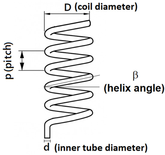
Figure 1.
Main geometrical parameters of the HCT.
The following section describes the results obtained over the last decade for predicting two-phase frictional pressure drops, highlighting which parameters have been considered to characterize the phenomena influencing the pressure drops.
2.1. Colombo et al.
Colombo et al. [1] proposed a correlation based on the L-M method [7], developed for horizontal straight pipes. This correlation, summarized in Table 1, extends the L-M approach by replacing the liquid pressure drop multiplier ϕ2LM, valid for straight pipes, with a modified multiplier ϕ2c that incorporates correction factors based on the mixture-to-liquid density ratio and the Dean number, a dimensionless quantity used in fluid mechanics to characterize flow in curved pipes or channels. As well known, a higher Dean number indicates stronger secondary flows and more pronounced centrifugal effects, while a lower Dean number implies the flow is closer to straight-pipe behavior.

Table 1.
Two-phase flow frictional pressure drop correlations valid for helical pipe.
It should be noted that the parameter ϕ2LM is determined using the correlation reported in [7], where the constant C depends on the flow regime (e.g., C = 20 for turbulent flow). The liquid pressure drop, (dP/dz)l, is evaluated using the only-liquid approach (i.e., considering only the liquid fraction of the mass flux) with the correlation of Ito [8], which has been shown to provide excellent agreement with experimental data for single-phase flow in helical pipes across various geometries and operating conditions, for both laminar and turbulent regimes.
The model was applied in [1] against experimental data covering pressures from 20 to 60 bar, mass fluxes from 200 to 800 kg/m2s, and steam qualities ranging from greater than 0 to less than 1.
2.2. Ferraris and Marcel
In their study, Ferraris and Marcel [2] calculated the two-phase frictional pressure gradient by applying the homogeneous equilibrium model and estimating the friction factor fTP.
Within this formulation, pressure and mass flux effects are largely captured by the kinetic energy term, with thermodynamic quality dependence handled through fTP. On this basis, the authors derived the correlations reported in Table 1, constrained to reproduce the single-phase Ito correlation at thermodynamic qualities of 0 and 1, and calibrated against experimental data. Accordingly, the liquid and gas friction factors are evaluated by treating the total mass flux G as if the flow consisted solely of liquid or solely of gas.
Their model was validated for pressures from 0.5 to 8 MPa, mass fluxes from 150 to 1100 kg/m2s, and steam qualities ranging from 0 to 1.
2.3. Moradkhani et al.
Moradkhani et al. [3] employed machine learning techniques combined with extensive experimental data to improve the accuracy of fTP predictions in smooth helically coiled tube heat exchangers. Six key dimensionless parameters were identified as most relevant for the description of flow behavior (Table 1):
- It = Tan(γ/2) is the inclination factor, γ is 0 for horizontal, −π/2 for vertical downflow, and +π/2 for vertical upflow;
- Pred = P/Pcritical is the reduced pressure evaluated as ratio of the pressure system to the critical pressure;
- X is the L-M parameter;
- Reₗₒ and Regₒ are the liquid-only and gas-only Reynolds number, respectively;
- δ = d/D is the curvature ratio, where d is the tube diameter and D is the coil diameter.
The correlation was validated for different working fluid, liquid-phase Reynolds numbers between 3592 and 143,266, vapor-phase Reynolds numbers between 55,143 and 811,688, reduced pressures in the range 0.034–0.325, inclination factors between −1 and +1, and L-M parameter ranging from 0.006 to 2.76 [3].
2.4. Su et al.
Su et al. [5] conducted new experiments on helically coiled pipes with a large curvature ratio (δ = 0.109) and combined their data with previous databases. Twenty-five existing correlations were tested against this dataset, but none provided satisfactory accuracy across all conditions. To overcome these limitations, the authors proposed a new correlation derived from the L–M approach, introducing a correction factor to account for differences among liquid, gas, and two-phase friction factors (see Table 1).
The resulting correlation achieves a broad applicability range (0.35–8 MPa, 200–1100 kg/m2s, 0.03–0.99 steam quality).
2.5. Giardina and Lombardo
Giardina and Lombardo [6] applied Cluster Analysis (CA) to a wide experimental dataset, aiming to group similar experimental cases and to uncover the dependencies among the main parameters.
As well known, CA is a statistical method that classifies a set of data into groups (clusters) based on their similarities, ensuring that data points within the same cluster share common characteristics while being distinct from those in other clusters [9]. This approach allows researchers to identify hidden trends, highlight relationships among variables, and capture dependencies that may not be immediately evident in complex experimental datasets.
The procedure was implemented through an R-CRAN script using the k-means clustering method [10]. The optimal number of clusters was identified by means of the Silhouette index [11], which provided an assessment of cluster cohesion and separation, ensuring a statistically consistent classification.
Once the clusters were defined, the correlation parameters were optimized through the least squares method combined with the BFGS (Broyden–Fletcher–Goldfarb–Shanno) algorithm [12] in order to minimize the Root Mean Square Error (RMSE) between experimental and predicted values. The final correlation is reported in Table 1.
It should be emphasized that the key parameters in the evaluation of ftp resulted from a combination of those employed in the correlations proposed by Ferrarirs [2] and Moradkhani [3]. Moreover, the Dean number is here modified through the introduction of a diameter Dc = D [1 + tan(β)]. This formulation accounts for the helical geometry, meaning that the Dean number implicitly reflects the influence of the helix pitch through the dependence on the angle β. As reported by the authors, the resulting correlation is applicable over a pressure range of 0.1–8 MPa and a mass flow rate of 70–2500 kg/m2s.
3. Models Validation Against Experiments
3.1. Experimental Data at Pressure from 0.1 to 0.4 MPa and Curvature Ratio of 0.012 and 0.01875
The helical pipes analyzed in this study consist of two tubes with coil diameters, D, of 0.64 m and 1 m, and pitches of 0.485 m and 0.79 m, respectively, while both have an inner diameter of 0.012 m [13]. Accordingly, the curvature ratios, δ, are 0.01875 and 0.012.
The two-phase flow experiments, provided to our group within the framework of a scientific collaboration, were conducted at mass flow rates between 800 and 2050 kg/m2s under operational pressures ranging from 0.1 to 0.4 MPa. The experiments involved a large number of air–water flow rate combinations. Pressure drop measurements were performed using nine taps on the coiled tubes, in combination with eight differential pressure transducers. The measurement uncertainty has been estimated to be below 5%.
The results are shown in Figure 2, Figure 3, Figure 4, Figure 5 and Figure 6, where the two-phase FPD experimental data, expressed in Pa, are compared with predicted values using the correlations proposed by Colombo [1] (Figure 2), Ferraris [2] (Figure 3), Moradkhani [3] (Figure 4), Su [5] (Figure 5), and Giardina [6] (Figure 6) for coil diameters of 0.64 m and 1 m, respectively.
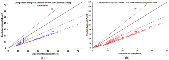
Figure 2.
Comparison of Colombo (2015) correlation predictions with the experimental data [13] for coil diameters of (a) 0.64 m (blue triangle symbols) and (b) 1 m (red circle symbols).
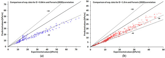
Figure 3.
Comparison of Ferraris (2020) correlation predictions with the experimental data [13] for coil diameters of (a) 0.64 m (blue triangle symbols) and (b) 1 m (red circle symbols).
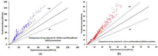
Figure 4.
Comparison of Moradkhani (2021) correlation predictions with the experimental data [13] for coil diameters of (a) 0.64 m (blue triangle symbols) and (b) 1 m (red circle symbols).
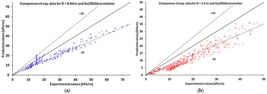
Figure 5.
Comparison of Su (2024) correlation predictions with the experimental data [13] for coil diameters of (a) 0.64 m (blue triangle symbols) and (b) 1 m (red circle symbols).
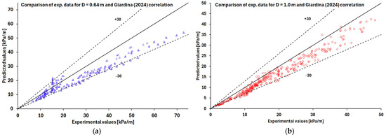
Figure 6.
Giardina (2025) correlation predictions with the experimental data [13] for coil diameters of (a) 0.64 m (blue triangle symbols) and (b) 1 m (red circle symbols).
Based on the analysis of the results, the best predictions are obtained by applying Ferraris correlation (Figure 3) and the one proposed by Giardina (Figure 6). The Giardina correlation produces errors below, or at most around 30% for most of the examined cases, for both diameters D = 0.64 m and D = 1 m, while the Ferraris correlation predicts pressure drops with errors of around 30%.
The Colombo correlation underestimates the experimental data with errors exceeding 30% (Figure 2), whereas the Moradkhani correlation overestimates the data with errors greater than 30% (Figure 4), while the Su correlation allows predictions within 30% only for experiments with D = 0.64 m (Figure 5a).
3.2. Experimental Data at 2.14 MPa and Curvature Ratio of 0.0246
The helically coiled tube test section used by Kozeki et al. [14] consists of a tube with an inner diameter of 15.5 mm, coil diameter, D, of 628 mm; thus, the curvature ratio, d, is of 0.0246. The operational pressure is 2.14 MPa with mass flow rates of 161, 325, and 486 kg/m2s.
The two-phase FPD experimental results, expressed as pressure drops in kPa/m as a function of vapor quality, are shown in Figure 7 with an error bar of ±15%.
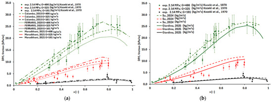
Figure 7.
Comparison among (a) correlations [1,2,3], (b) correlations [5,6] with experimental data [14].
In particular, Figure 7a compares the experimental data with the predictions of Colombo [1], Ferraris [2], and Moradkhani [3], while Figure 7b shows the comparison with the predictions of Su [5] and Giardina [6].
The dispersion of experimental measurements shows that the correlations perform similarly overall. Nevertheless, at higher flow rates, Giardina and Su correlations provide the closest agreement with the observed pressure drops (Figure 7b).
The Colombo and Ferraris correlations underestimate pressure drops at the highest mass flux of 486 kg/m2s and vapor quality values above 0.45, while the Moradkhani correlation provides very good predictions.
3.3. Experimental Data at Pressures from 2 to 6 MPa and Curvature Ratio 0.01253
The test section is a 32 m long helically coiled pipe, characterized by an inner diameter of 0.01253 m, a coil diameter of 1 m, a curvature ratio, d, of 0.01253, and a pitch of 0.8 m [1]. Nine pressure taps are installed at 4 m intervals. Two-phase flow experiments were performed in both adiabatic and diabatic regimes, with mass fluxes of 200–800 kg/m2s, pressures of 2–6 MPa, and qualities between 0.1 and 0.9. The measurement uncertainty has been estimated to be below 3.5%.
Table 2 reports some results in terms of Root Mean Squared Error (RMSE) and Mean Absolute Percentage Error (MAPE), in percentage, for the various correlations.
Table 2.
RMSE and MAPE calculated for different correlations based on experimental data [1].
From Table 2, it is possible to highlight the following: Ferraris [2] generally shows low RMSE and MAPE values (RMSE and MAPE below 15%). Colombo [1] shows relatively high RMSE (16–26%) and MAPE (14–19%) across most operating conditions. Giardina [6] exhibits good performance across all mass fluxes and pressures, with RMSE and MAPE below 13%. Su [5] provides reasonable predictions at lower mass fluxes (G = 200–400 kg/m2s), with RMSE between 7.7% and 16% and MAPE between 5.4% and 14.5%, but its errors tend to increase at higher mass fluxes (G = 600–800 kg/m2s). Moradkhani [3] shows high errors in specific cases (e.g., G = 600 kg/m2s, P = 4 MPa, RMSE = 49.1%, MAPE = 30.1%; G = 800 kg/m2s, P = 2 MPa, RMSE = 42.6%, MAPE = 28.7%), while in other conditions the errors are lower, with RMSE generally below 25% and MAPE below 15%.
3.4. Experimental Data at 7 MPa and Curvature Ratio of 0.107
According to [5], the test section consists of a helically coiled pipe 5.28 m long, with an inner diameter of 12 mm, coil diameter of 112 mm (δ = 0.107), and a pitch of 22.5 mm. System pressures ranged from 3.5 to 7 MPa, and mass fluxes from 320 to 1100 kg/m2s. The authors in [5] reported that the maximum uncertainty of the frictional pressure drop gradient is about 7.17%.
Figure 8 compares predictions with two-phase FPD data at 320, 550, 800, and 1100 kg/m2s and reports the error bar of 7%.

Figure 8.
Comparison between predicted correlations and measured data [1,2,3,4,5]. The tests were conducted at an operating pressure of 7 MPa and mass fluxes of (a) 320 kg/m2s, (b) 550 kg/m2s, (c) 820 kg/m2s, and (d) 1100 kg/m2s.
Table 3 summarizes the results of the different correlations examined in terms of RMSE and MAPE, expressed as percentages.
Table 3.
RMSE and MAPE calculated for different correlations based on experimental data [5].
The Colombo correlation [1] consistently overestimates the experimental data, with RMSE values around 85–97% and MAPE exceeding 69%, regardless of the mass flux. Ferraris [2] and Moradkhani [3] perform significantly better than Colombo [1], with RMSE ranging from 18% to 27% and MAPE from 14% to 22% across all mass fluxes. Su [5] provides relatively low errors at lower mass fluxes (320–820 kg/m2s), with RMSE around 12–15.0% and MAPE 9.4–13.0%, but its accuracy decreases at the highest mass flux (1100 kg/m2s, RMSE = 33.6%, MAPE = 19.1%). Giardina [6] demonstrates the best overall predictive performance, with RMSE ranging from 7.0% to 11.8% and MAPE between 6.2% and 10.7%.
3.5. Comparison Results
It is worth noting that some of the experimental data used for comparison exceed the validity ranges of certain correlations. While these comparisons are presented for completeness and illustrative purposes, the correlations are not necessarily expected to provide accurate predictions outside their specified applicability ranges. However, this study allows us to offer important insights into the trends and relative performance of the correlations.
By combining all experimental data with the corresponding predictions from the correlations examined in this study (Table 4), the two one-sided tests (TOSTs) [15] was performed to assess the equivalence between datasets within a predefined margin, set here at 30% of the data mean. The TOST procedure involves two one-sided tests:
- p_lower checks whether the mean difference is not lower than −30%;
- p_upper checks whether the mean difference is not higher than +30%.
Table 4.
Results of the TOST and MAPE using all experimental data and predicted values examined in this paper.
Table 4.
Results of the TOST and MAPE using all experimental data and predicted values examined in this paper.
| Correlation | p_lower | p_upper | Equivalent (SL = 0.05) | MAPE (%) |
|---|---|---|---|---|
| Colombo [1] | 8.85725 × 10−210 | 1 | NO | 32.29 |
| Ferraris [2] | 4.59264 × 10−230 | 1 | NO | 19.96 |
| Moradkhani [3] | 1 | 4.6142 × 10−161 | NO | 45.32 |
| Su [5] | 3.72241 × 10−250 | 1 | NO | 23.27 |
| Giardina [6] | 6.12354 × 10−249 | 0.00287597 | YES | 14.78 |
In this context, the significance level (SL) is set at 0.05. A p-value below this threshold provides sufficient evidence that the observed difference lies within the equivalence margin, indicating that the datasets can be considered equivalent. Equivalence is concluded if both p-values are below 0.05; otherwise, the margin is exceeded and the datasets are deemed not equivalent.
The analysis of the TOST results reveals that, among the models considered, only Giardina [6] exhibits both p_lower and p_upper values below the significance threshold of 0.05. This indicates that the differences between the two data series fall within the predefined tolerance margin, suggesting a strong ability to reproduce the experimental values. This interpretation is further supported by the MAPE value of 14.78%, the lowest among those reported, which reflects a relatively small mean percentage error and therefore a higher predictive accuracy.
The models of Colombo [1], Ferraris [2], Moradkhani [3], and Su [5] do not meet the equivalence condition, as at least one of the TOST tests yields a p-value greater than 0.05. This implies that, for these models, the differences between observed and predicted values exceed the established statistical tolerance margin.
Nevertheless, the degree of deviation varies considerably: the Ferraris [2] model shows a MAPE of 19.96%, indicating better performance compared with Colombo [1] (32.29%), Su [5] (23.27%), and especially Moradkhani [3], which displays the highest error (45.32%).
The underestimation of Colombo et al.’s correlation can be explained by the fact that it is derived from the L–M approach, originally developed for straight tubes, and that the model was adapted to only one value of the curvature ratio (see Table 1). This highlights a limited capability of the correlation to account for curvature-induced secondary flows, which are generally represented by the Dean number.
This highlights a limited capability of the correlation to account for curvature-induced secondary flows, as characterized by the Dean number.
The correlations of Ferraris and Su, defined for a wide range of curvature ratios and operating pressures, tend to overestimate the experimental data, although with relatively small deviations, as previously noted. This overestimation is likely mainly due to their application at operating pressures below 0.35 MPa, thus outside the validity range reported in Table 1. It is worth noting that the experimental data examined in Section 3.1 were primarily characterized by slug and plug flow regimes, with transitions to bubbly or churn regimes. Furthermore, strong interactions between the different regimes were observed, which can reduce the impact on pressure drops compared to those observed under higher flow rate and pressure conditions.
The overestimation produced by the Moradkhani correlation suggests that the machine learning model overemphasizes curvature and pressure effects, which become dominant at relatively low system pressures (0.1–0.4 MPa).
It should be noted that in the Moradkhani model the dependence on the Reynolds number is considered separately from the curvature ratio parameter, while it is well known that the Dean number combines both contributions. This could impact the model’s ability to accurately predict low-pressure operating conditions.
The Giardina correlation performs best because the CA allows grouping experimental cases based on their similarities and identifying dependencies among the main physical and geometrical parameters. This likely enabled an improved and extended use of the parameters already employed in the other correlations examined in the study, including a modified Dean number that accounts also the helical pitch.
4. Conclusions
This study compared several literature correlations from the last decade for predicting two-phase frictional pressure drops in helically coiled pipes, validating their performance against extensive experimental datasets. The main findings can be summarized as follows:
- Ferraris correlation [2] shows the highest agreement with all experimental data. However, the predictions appear more sensitive to changes in the curvature ratio and become less accurate as the flow rate increases.
- Moradkhani correlation [3] showed large deviations from the experimental data for different curvature ratios and operating pressures.
- Su correlation [5] performs with errors comparable to the Ferraris correlation. However, accuracy decreases at a mass flow rate of 1100 kg/m2s, pressure of 7 MPa, and high curvature ratios (δ = 0.107), where RMSE rises to about 33% (see Table 3). At pressures below 0.4 MPa and curvature δ = 0.01875, the experimental data exhibit large scatter around an average error of approximately −30% (Figure 5b).
- Giardina correlation [6] demonstrated a good reliability, with errors generally within 30% across the full range of operating pressures, mass, and curvature ratios examined in this paper.
In conclusion, Giardina and Ferraris correlations provide the best compromise between accuracy and applicability range, making it a reliable tool for the design and optimization of helical coil steam generators, with particular relevance for advanced modular nuclear reactors and other high-performance energy systems.
It is worth noting that several experimental datasets are available for pressures higher than 2 MPa and for different helical curvature ratios, allowing a detailed analysis of the trends in two-phase frictional pressure drops. However, at lower pressures, experimental data are limited to only a few curvature ratios. Therefore, future studies could focus on this low-pressure range to provide a more comprehensive validation of the proposed correlations.
Author Contributions
Conceptualization, M.G.; methodology, M.G.; validation, M.G. and C.L.; formal analysis, M.G. and C.L.; writing—original draft preparation, M.G.; writing—review and editing, M.G. and C.L. All authors have read and agreed to the published version of the manuscript.
Funding
This research received no external funding.
Data Availability Statement
No new data were created or analyzed in this study. Data sharing is not applicable to this article.
Acknowledgments
The authors gratefully acknowledge Politecnico di Torino and Politecnico di Milano for providing the experimental data used in this study. These data greatly enhanced the quality and robustness of our analyses and contributed to the reliability of the results presented.
Conflicts of Interest
The authors declare no conflicts of interest.
Nomenclature
| Acronyms | |
| CA | Cluster Analysis |
| FPD | Frictional Pressure Drop |
| HCT | Helically Coiled Tube |
| L-M | Lockhart–Martinelli |
| MAPE | Mean Absolute Percentage Error |
| RMSE | Root Mean Squared Error |
| SL | Significance Level |
| TP | Two-Phase |
| TOST | Two One-Sided Tests |
| Notation | |
| d | Inner tube diameter (m) |
| D | Coil diameter (m) |
| De | Dean number (−) |
| f | Frictional factor (−) |
| G | Mass flux (kg/m2s) |
| P | System pressure (Pa) |
| p | Picth (m) |
| Re | Reynolds number (−) |
| x | Steam quality (−) |
| It | Tube inclination factor tg(γ/2) |
| Subscript | |
| c | Coil |
| g | Gas or steam |
| go | Gas-only |
| l | Liquid |
| lo | Liquid-only |
| m | Homogeneous model |
| red | Reduced pressure |
| Greek symbols | |
| β | Helix angle |
| δ | Curvature ratio d/D |
| γ | Inclination angle: 0 horizontal, −π/2 vertical downflow, +π/2 vertical upflow |
| μ | Dynamic viscosity (Pa s) |
| ϕ | Pressure drop multiplier (−) |
| ρ | Density (kg/m3) |
| X | Martinelli parameter (−) |
References
- Colombo, M.; Colombo, L.P.; Cammi, A.; Ricotti, M.E. A scheme of correlation for frictional pressure drop in steam–water two-phase flow in helicoidal tubes. Chem. Eng. Sci. 2015, 123, 460–473. [Google Scholar] [CrossRef]
- Ferraris, D.L.; Marcel, C.P. Two-phase flow frictional pressure drop prediction in helical coiled tubes. Int. J. Heat Mass Transf. 2020, 162, 120264. [Google Scholar] [CrossRef]
- Moradkhani, M.A.; Hosseini, S.H.; Mansouri, M.; Ahmadi, G.; Song, M. Robust and universal predictive models for frictional pressure drop during two-phase flow in smooth helically coiled tube heat exchangers. Sci. Rep. 2021, 11, 20068. [Google Scholar] [CrossRef] [PubMed]
- Giardina, M.; Buffa, P. Simulations of single and two-phase flows through helical tubes with different geometries and mass flow rates. J. Phys. Conf. Ser. 2025, 1742, 6596. [Google Scholar] [CrossRef]
- Su, Y.; Li, X.; Wu, X. Frictional pressure drop correlation of steam-water two-phase flow in helically coiled tubes. Ann. Nucl. Energy 2024, 208, 110764. [Google Scholar] [CrossRef]
- Giardina, M.; Lombardo, C. A generalized correlation for pressure drop prediction in helically coiled tubes across different geometries and operating conditions. In Proceedings of the UIT2025-42nd International Heat Transfer Conference, Florence, Italy, 23–25 June 2025. [Google Scholar]
- Lockhart, R.W.; Martinelli, R.C. Proposed correlation of data for isothermal two-phase two-component flow in pipes. Chem. Eng. Prog. 1949, 45, 39–48. [Google Scholar]
- Ito, H. Friction factors for turbulent flow in curved pipes. ASME J. Basic Eng. Trans. 1959, 81, 123–134. [Google Scholar] [CrossRef]
- Kaufman, L.; Rousseeuw, P.J. Finding Groups in Data: An Introduction to Cluster Analysis; Wiley-Interscience: New York, NY, USA, 1990. [Google Scholar]
- MacQueen, J. Some methods for classification and analysis of multivariate observations. In Proceedings of the Fifth Berkeley Symposium on Mathematical Statistics and Probability; University of California Press: Berkeley, CA, USA, 1967; Volume 1, pp. 281–297. [Google Scholar]
- Rousseeuw, P.J. Silhouettes: A graphical aid to the interpretation and validation of cluster analysis. J. Comput. Appl. Math. 1987, 20, 53–65. [Google Scholar] [CrossRef]
- Nocedal, J.; Wright, S.J. Numerical Optimization, 2nd ed.; Springer: New York, NY, USA, 2006. [Google Scholar]
- Orio, M. Fluidodinamica Bifase in Condotti Elicoidali per Applicazioni Nucleari. Ph.D. Thesis, Politecnico di Torino, Torino, Italy, 2013. [Google Scholar]
- Kozeki, M.; Nariai, H.; Furukawa, T.; Kurosu, K. A study of helically-coiled tube once-through steam generator. Bull. JSME 1970, 13, 1485–1494. [Google Scholar] [CrossRef]
- Wellek, S. Testing Statistical Hypotheses of Equivalence and Noninferiority; CRC Press: Boca Raton, FL, USA, 2010. [Google Scholar]
Disclaimer/Publisher’s Note: The statements, opinions and data contained in all publications are solely those of the individual author(s) and contributor(s) and not of MDPI and/or the editor(s). MDPI and/or the editor(s) disclaim responsibility for any injury to people or property resulting from any ideas, methods, instructions or products referred to in the content. |
© 2025 by the authors. Licensee MDPI, Basel, Switzerland. This article is an open access article distributed under the terms and conditions of the Creative Commons Attribution (CC BY) license (https://creativecommons.org/licenses/by/4.0/).