Abstract
The molten salt reactor (MSR) is a prominent Generation IV nuclear reactor concept that offers substantial advantages over conventional solid-fueled systems, including enhanced fuel utilization, inherent passive safety features, and significant reductions in long-lived radioactive waste. Central to its safety strategy is a reliance on natural circulation (NC) mechanisms, which eliminate the need for active pumping systems and enhance system reliability during normal and off-normal conditions. However, the challenges associated with molten salts, such as their high melting points, corrosivity, and material compatibility issues, render experimental investigations inherently complex and demanding. Therefore, the use of high-Pr-number surrogate fluids represents a practical alternative for studying molten salt behavior under safer and more accessible experimental conditions. In this study, a single-phase natural circulation loop setup at the University of Idaho’s Thermal–Hydraulics Laboratory was employed to investigate NC behavior under various operating conditions. The RELAP5-3D code was initially validated against water-based experiments before employing Therminol-66, a high-Prandtl-number surrogate for molten salts, in the natural circulation loop for the first time. The RELAP5-3D results demonstrated good agreement with both steady-state and transient experimental results, thereby confirming the code’s ability to model NC behavior in a single-phase flow regime. The results also highlighted certain experimental limitations that should be addressed to enhance the NC loop’s performance. These include increasing the insulation thickness to reduce heat losses, incorporating a dedicated mass flow measurement device for improved accuracy, and replacing the current heater with a higher-capacity unit to enable testing at elevated power levels. By identifying and addressing the main causes of these limitations and uncertainties during water-based experiments, targeted improvements can be implemented in both the RELAP5 model and the experimental setup, thereby ensuring that tests using a surrogate fluid for MSR analyses are conducted with higher accuracy and minimal uncertainty.
1. Introduction
The Generation IV International Forum (GIF) was established as an international collaborative project to conduct research on fourth-generation nuclear systems. Its goal is to assess the feasibility and performance of these systems and make them available for industrial use by 2030. The GIF has identified six reactor technologies for further research and development: the gas-cooled fast reactor (GFR), the lead-cooled fast reactor (LFR), the molten salt reactor (MSR), the sodium-cooled fast reactor (SFR), the supercritical-water-cooled reactor (SCWR), and the very-high-temperature reactor (VHTR) [1]. Molten salt reactors (MSRs) were primarily developed at Oak Ridge National Laboratories (ORNL) in the late 1940s. After nearly three decades of supported research and development, design progression led to the implementation of the single-fluid, graphite-moderated Molten Salt Breeder Reactor (MSBR) in the late 1960s [2,3,4].
MSRs have various operational and safety advantages, such as their ability to automatically drain fuel to passively cooled, critically safe dump tanks, their continuous removal of fission products, and their lack of any “dead time” after shutdown or power decrease. MSRs also require only a low-pressure vessel and have strong negative temperature and void coefficients for safety. Additionally, MSRs use molten fluoride salts as coolants, which have a higher volumetric heat capacity than pressurized water reactors (PWRs) and lower thermal conductivity than sodium. They also produce significantly less transuranic waste and can achieve break-even breeding with ease. Furthermore, terrestrial thorium is more abundant than uranium, making the Th–U fuel cycle an attractive option for MSRs [5,6]. Although the literature on molten salt reactors (MSRs) is extensive, it has been comprehensively addressed in our prior work [7,8]. Given that the present study focuses on single-phase natural circulation loops (SPNCLs) specifically designed for investigating molten salts, the literature review herein is restricted to studies directly related to such loop configurations.
Many studies have been conducted to investigate natural circulation (NC) behavior using various test loops under different operating conditions. A theoretical investigation of a natural circulation loop (NCL) with a point heat source and a point heat sink explained the occurrence of instability by proposing a theory based on the transport of warm and cold fluid pockets. These pockets are generated at the heater and cooler, respectively, and their movement within the loop influences the system’s stability [9]. An experimental study was conducted to investigate the steady-state behavior of an SPNCL with a vertical heater and vertical cooler configuration (VHVC) [10]. The experiment covered a wide range of operating conditions through 29 steady-state tests. The results were compared with a developed 1D model based on the NCL, leading to the conclusion that the model can reliably achieve steady-state solutions for various operating conditions. Furthermore, it can be used to obtain precise steady-state solutions for SPNC loops across different configurations and working conditions. Multi-loop experimental data under steady-state, single-phase conditions were used to validate the system model in the RELAP5/SCDAPSIM/MOD 4.0 code [11]. The experiment consists of three loops, two of which operate on NC, while the third operates on forced circulation. The experimental loop successfully established NC under various pressure conditions. An experimental study was carried out to investigate the flow phenomena in an SPNCL [12]. The effects of temperature and heating power variations at low system pressure on flow characteristics were studied. RELAP5/MOD3.2 has been used to simulate the steady-state, transient, and stability behavior of natural circulation-based experimental facilities, such as the High-Pressure Natural Circulation Loop (HPNCL) and the Parallel Channel Loop (PCL) installed and operated at Bhabha Atomic Research Centre (BARC) [13]. Numerical and experimental studies were performed to investigate the flow reversal in an NCL at atmospheric pressure [14]. The results demonstrate that increasing the upstream pressure loss coefficient extends the boundaries of the stable flow region, enabling larger exit void fractions. In configurations with dominant upstream pressure losses, stable boiling points occur at high mass and heat fluxes. In contrast, larger downstream pressure loss coefficients lead to increased instability and flow reversal. A non-dimensional formula for an SPNCL was developed to simulate steady-state operation, where the entire loop follows a single friction law. Subsequently, a generalized flow equation that accommodates multiple friction laws was proposed, which exhibited strong predictive capability when compared to experimental data obtained from a uniform-diameter rectangular loop [15,16].
Several studies have investigated the behavior of NC using molten salt as the working fluid. Both experimental and theoretical approaches have been employed to examine the steady-state characteristics of molten salt natural circulation loops (MSNCLs) [17,18]. The analysis considered four different configurations of heater and cooler orientations, utilizing a 60:40 weight ratio mixture of sodium nitrate and potassium nitrate as the working fluid. The in-house one-dimensional LeBENC code has been validated using experimental data obtained from the previously mentioned MSNCL [19]. The results demonstrate that the LeBENC code is capable of predicting both steady-state and transient NC behavior in similar molten-salt-based systems. Verification and validation investigations were conducted for the system analysis module (SAM) code using analytical solutions and experimental data from the Compact Integral Effects Test (CIET) experimental loop for both forced and natural circulation flow [20,21]. It is important to note that stability analysis is a crucial aspect that must be carefully addressed to ensure reliable and stable NC flow in SPNCLs with different heaters and cooler configurations [22,23,24]. The effects of various modeling assumptions on the steady-state and transient performance of a single-phase natural circulation loop have been analyzed. This study was based on a configuration with a vertical heater and a horizontal cooler (VHHC) [25]. NC is extensively used in Generation IV reactors, including MSRs, to improve their safety and reliability. The validation of numerical codes plays a vital role in the development, assessment, and licensing of safety analyses for these reactor designs. Besides ensuring the accuracy of predictive models, code validation is fundamental to advancing the understanding and optimizing the application of NC in Generation IV reactor systems. The baseline for the current validated code using water as the working fluid is to evaluate the NC performance, which will then be compared to that of Therminol-66 as a surrogate fluid for molten salt [26]. Additionally, a broad range of Prandtl numbers should be examined to better assess the heat transfer characteristics of various fluids. Given the fact that the natural circulation loops discussed in the literature exhibit simple and varying design characteristics such as aspect ratio, cooler and heater configurations, and loop diameter, it is essential to investigate the NC behavior specific to the current design which exhibits a complex geometrical configuration and compare the findings with those of other natural circulation loops.
The present study investigates the behavior of a single-phase natural circulation loop (SPNCL) under various operating conditions, using water as the working fluid during the preliminary phase. Concurrently, the research aims to assess the capability of the RELAP5-3D system code to accurately simulate natural circulation phenomena under the tested conditions. A series of steady-state and transient experiments are conducted to validate the RELAP5-3D code. Also, the present analysis explores the limitations associated with both the experiment and the code before implementing the main surrogate fluid. In future, these findings will contribute to the broader R&D efforts supporting the design and development of molten salt reactors (MSRs).
2. Description of the Experimental Test Loop
2.1. Test Loop Design
The experimental loop, depicted in Figure 1, is made from 2.5-inch schedule 80 stainless steel 316 piping, with each section joined by 600-pound ring flanges. The loop includes two heaters, an immersion heater manufactured by the Watlow company [27], and a guard heater, located at its bottom left. The immersion heater has a power rating of 4000 W, while the guard heater collectively provides an additional 2000 W to this section. The system’s maximum heat input capability is 6000 W. However, due to limitations in the laboratory setup in which the experiments are conducted, the practical maximum power is closer to 5000 W. For the experiments conducted with water, the maximum heater power applied to the system was approximately 3000 W in order to prevent overheating and potential damage to the heater burning during transient scenarios.
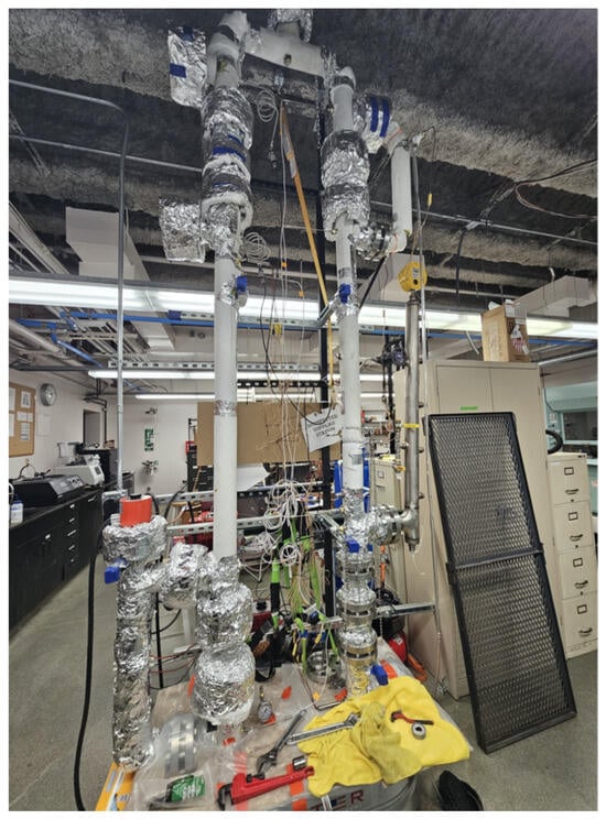
Figure 1.
A photograph of the NC experimental loop.
A cooler is situated at the top right of the loop. Below the heat exchanger, an L-shaped accumulator is incorporated, serving dual functions: facilitating the filling of the loop with liquid and accommodating thermal expansion as the temperature rises. This design helps to prevent sudden pressure increases within the loop. The cooler, referred to as the heat exchanger in the loop figures, is a shell-and-tube design. It consists of eight copper tubes through which the natural circulation flow passes, while cooling water flows counter to the primary fluid within the stainless-steel pipe shell. Each of the eight tubes is constructed from 1/4-inch tubing with an outer diameter of 0.38 inches and a length of 19 inches [28]. The test loop heater and the cooler tube bundle are shown in Figure 2a,b, respectively.
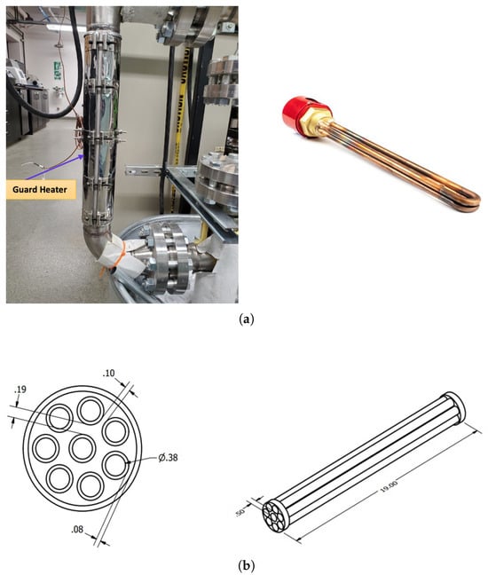
Figure 2.
Test loop heater and cooler details. (a) A 2000 W guard heater (left); a two-element immersion heater (right). (b) A schematic view of the tube plate of the heat exchanger (cooler) (left); tube bundle (right).
The cooling water loop consists of two 55-gallon barrels that serve as reservoirs for water supplied from the laboratory source. The barrels are heated to specific temperatures depending on the requirements of the experiment being conducted. Water is pumped from the barrels through a flow meter and into the shell side of the heat exchanger. After passing through the heat exchanger, the water is discharged into a drain. The main design parameters of the NCL are given in Table 1.

Table 1.
Test loop design parameters.
2.2. Piping and Instrumentation
The experimental loop was equipped with a range of instrumentation for monitoring and data acquisition. Three pressure transducers (PTs) and two pressure gauges (PGs) were installed to measure pressure at key locations. The transducers located at the bottom of the loop were rated for pressures up to 300 psig, while the transducer mounted in the accumulator had a maximum rating of 150 psig, adequately covering the expected pressure range during experiments. For temperature measurements, resistance temperature detectors (RTDs) were distributed throughout the loop, and two five-point thermocouples (TCs) were installed to capture a detailed thermal profile of the working fluid as it flowed through the system. Additionally, the loop piping and flanges were insulated with a 14–20 mm thick layer of ceramic glass to minimize heat loss and maintain thermal stability during operation. The instrumentation layout during the liquid-phase experiments is shown in Figure 3, while Figure 4 presents the piping and instrumentation diagram (P&ID) for the cooling water loop. Data acquisition for the loop experiments was performed with a sampling interval of 10 s, which was sufficient to capture transient behavior without overloading the LabVIEW 2024 Q3 software. The recorded data were subsequently exported into Python 3.9 for post-processing. Within Python, steady-state conditions were identified by applying a minimum criterion of 30–60 min of stable operation. Once a steady-state window was established, the corresponding data points were averaged using the arithmetic mean to determine representative values of loop temperatures, mass flow rate, and pressures. Each test was typically repeated once/twice to ensure repeatability, and retesting was only performed if boundary condition issues were observed, such as irregular cooling-water temperatures or heater power fluctuations.
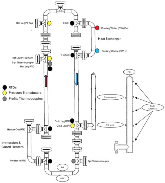
Figure 3.
P&ID of the natural circulation experimental loop with associated names of each instrumentation sensors.
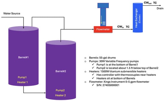
Figure 4.
Cooling water loop P&ID.
2.3. Calibration Process and Uncertainty Analysis
Equation (1) pertains to two pressure transducers that convert current (mA) to pressure (psig). These transducers are identified by part number Swagelok PTI-S-MG6-12AO [29]. Equation (2) corresponds to a calibrated pressure transducer from OMEGA, which also converts current (mA) to pressure (psig). This transducer is identified by part number OMEGA PX309 [30].
To calibrate the six RTDs and all associated thermocouples, fluke metrology wells were employed. Specifically, two models were utilized, namely the 9171-X-R and the 9173-X-R [31], which cover temperature ranges of –30 °C to 155 °C and 50 °C to 700 °C, respectively. The six RTDs and the two K-type profile thermocouples (i.e., the five-point thermocouples shown in Figure 3) were calibrated over a temperature range of 0 °C to 300 °C. Additionally, two K-type thermocouples used for measuring the inlet and outlet temperatures of the cooling water in the heat exchanger were calibrated over a narrower range of 0 °C to 50 °C. A total of eight calibration equations were derived for the RTDs, including two equations for each of the following locations: the heater, the cooler, the riser and downcomer, and the cooling water inlet and outlet. Table 2 summarizes the measurement uncertainties associated with the key devices employed in the test loop, including thermocouples, pressure transducers, flow meters, and power measurement systems. These uncertainties arise from factors such as sensor resolution, calibration drift, and data acquisition precision. As shown, temperature measurements exhibit uncertainties in the order of ±0.1–0.344 °C, while pressure and flow rate devices demonstrate relative uncertainties within a few percent of the measured value. Electrical power input, obtained from calibrated power ammeters, carries its own inherent uncertainty due to current and voltage measurement accuracy. Quantifying these uncertainties is essential for error propagation analysis and for assessing the confidence intervals of derived quantities such as heat balance, mass flow rate, and dimensionless parameters. Regarding the determination of mass flow rate on the primary side, it was calculated based on an energy balance across the cooler. By measuring the volumetric flow rate in the cooling water loop and the temperature difference between the inlet and outlet of the shell side of the cooler, the heat removed from the primary side was determined, allowing the corresponding mass flow rate to be inferred.
Table 2.
Measurement devices and associated uncertainties in the NCL.
2.4. Experimental Procedure
The following procedures were followed during the experimental campaign. The water loop needed to be refilled approximately every ten days, which was carried out by pumping water into the accumulator port—typically one day prior to the scheduled experiment. On the day of the experiment, the cooling water loop was initiated by opening the water source, allowing flow into collection barrels and subsequently to a drain until thermal equilibrium was achieved. Once a stable inlet temperature was reached, the cooling water was circulated through the cooler. Each experimental run began by applying an initial power using the combination of a guard and immersion heater. The loop was operated until a steady-state condition was established, defined by an average temperature slope of approximately °C/s over a 30 min period. In selected experiments, after reaching this initial steady state, one or more boundary conditions such as the cooling water flow rate, cooling water inlet temperature, or heater power were modified, and the system was allowed to stabilize again under the new conditions. The experimental campaign included five single-power transient tests conducted at fixed heater power levels of 400 W, 800 W, 1000 W, 2000 W, and 3000 W. An additional experiment maintained a constant heater power of 800 W, followed by a slight reduction in the cooling water inlet temperature after a steady state was achieved. In a similar test, the heater was initially operated at 800 W, and the cooling water inlet temperature was reduced. Once a noticeable rise in the heater inlet temperature was observed, the heater power was increased to 900 W to examine the dynamic thermal response.
Two further runs at 2000 W and 3000 W involved shutting down the cooling water loop after achieving a steady state. When the heater temperature approached the maximum allowable limit of 280 °C, the cooling water flow was reinstated, and the system was allowed to settle into a new steady state. In addition, a multi-step power transient experiment was performed, starting at 1000 W, increasing to 2000 W, and then stepping up to 3000 W to evaluate the system’s response to sequential power increases. At the end of each experiment, the system was shut down by turning off all active heaters. Residual cooling water in the barrels was pumped through the cooler to remove remaining heat, and once the water supply was depleted, the loop was left to cool naturally via convection to the temperature of the ambient environment.
3. Theoretical Analysis of SPNCL
The natural circulation (NC) phenomenon arises from density gradients induced by temperature differences between the hot and cold legs of the loop. Three fundamental elements govern the NC process: (i) the presence of a heat source and a heat sink, (ii) the influence of gravity, and (iii) an appropriate geometrical configuration to sustain circulation. Natural circulation can occur under both single-phase and two-phase flow conditions. The present study focuses specifically on single-phase natural circulation (SPNC). Under this assumption, the steady-state flow rate can be theoretically determined using fundamental conservation equations. For a closed-loop system with an incompressible fluid, the conservation of mass and energy is expressed as follows:
where , and are the mass flow rate, fluid density, fluid velocity, cross-sectional area, power, and specific enthalpy for the hot and cold leg, respectively. To establish sufficient conditions for a steady-state NC flow inside the loop, the driving force should be balanced with the resistance force, which implicitly comes from the integration of the momentum balance over the entire loop. The thermal driving head can be calculated using the difference in hydrostatic pressures:
The resistance force can be decoupled into two components, namely the (i) frictional pressure drop and (ii) local pressure losses (form losses), as follows:
where f, L, K, and D are the friction factor, length, local pressure drop coefficient, and pipe diameter, respectively. The friction factor can be determined by the following equation based on the flow regime:
For a circular pipe, the Reynolds number is given by
The heat transfer from the heater to the working fluid is given by
The heater efficiency can be determined by the ratio between thermal and electrical power as follows:
Finally, the average temperature inside the loop is given by:
4. RELAP5-3D Modeling
The RELAP5 code is a best-estimate, one-dimensional (1-D), non-equilibrium, transient, two-fluid model developed for solving problems involving mixtures of water and steam [32]. RELAP5-3D is the latest version in the RELAP5 series developed at Idaho National Laboratory (INL) and is used for analyzing transients and accidents in water-cooled nuclear power plants and related systems, as well as for advanced reactor designs [33]. RELAP5-3D evolved from the 1D RELAP5/MOD3 code, with its most notable feature being the fully integrated, multi-dimensional thermal–hydraulic and kinetic modeling capability that sets it apart from its predecessors.
4.1. RELAP5 Code Field Equations
The basic field equations for the two-fluid non-equilibrium model consist of two phasic continuity equations, two phasic momentum equations, and two phasic energy equations. These equations are expressed in differential stream tube form, with time and one spatial dimension as independent variables, and are formulated in terms of time and volume-averaged dependent variables. Therefore, the RELAP5 model solves the field equations for seven primary dependent variables: pressure (p), phasic specific internal energies ( and ), vapor volume fraction (), phasic velocities ( and ), and non-condensable quality (). The phasic continuity equations for both vapor and liquid, respectively, can be represented as follows:
where is the total mass transfer at the vapor–liquid interface. The momentum equations for vapor and liquid, respectively, are given by
The terms FIG and FWG represent the interface and wall frictional drag, respectively, which is linear with respect to velocity. These terms are the product of the friction coefficient, the frictional reference area per unit volume, and the magnitude of the fluid velocity. The energy conservation equation for the vapor and liquid phases is as follows:
where and are the interface energy transfer terms for liquid and vapor, and are the wall heat transfer rates per unit volume, and and are the dissipation energy terms for the liquid and vapor phase, respectively. The non-condensable gas equation can be represented by
4.2. RELAP5-3D Nodalization
For the purpose of code validation, a nodalization diagram representing the experimental loop geometry with appropriate fidelity is illustrated in Figure 5. The hydrodynamic model is discretized into control volumes (CVs) corresponding to physical sections of the system. Both the heater and the shell-and-tube heat exchanger (cooler) are subdivided into eight nodes each, providing sufficient spatial resolution for capturing thermal and flow gradients. The accumulator is modeled using a branch component (B440) to regulate the loop pressure. Piping sections are represented using PIPE components, each subdivided into a series of control volumes with appropriately selected node sizes to ensure numerical stability and physical accuracy. Component connectivity is achieved using single junctions (SNGLJUN), while time-dependent junctions (TMDJ) are employed to impose specified mass flow rates. Time-dependent volumes (TMDV) serve as pressure boundary conditions at the inlet and outlet of the cooler. The hydrodynamic components are numbered in accordance with the flow direction, which is clockwise. Specifically, PIPE P110 represents the heater (heat source), P140 (25 CVs) models the riser (hot leg), and P180 corresponds to the tube side of the heat exchanger. The downcomer (cold leg) is modeled using P220 and P230. On the secondary side, P320 represents the shell side of the heat exchanger, while TMDV300 and TMDV330 define the inlet and outlet boundaries of the cooling loop, respectively. Heat structures (HS) are defined to model heat addition and removal. The applied heater power is modeled by HS1110, whereas HS1180 accounts for heat exchange between the primary and secondary sides of the heat exchanger. Additionally, heat losses to the environment are simulated by incorporating an insulation layer composed of ceramic glass, with a thickness ranging from 14 to 20 mm. The local pressure losses in the loop were determined based on the specific design characteristics of the piping system. These include factors such as bends, fittings, valves, expansions, contractions, and surface roughness, which contribute to localized flow resistance. Table 3 summarizes the lengths of each part in the nodalization diagram.
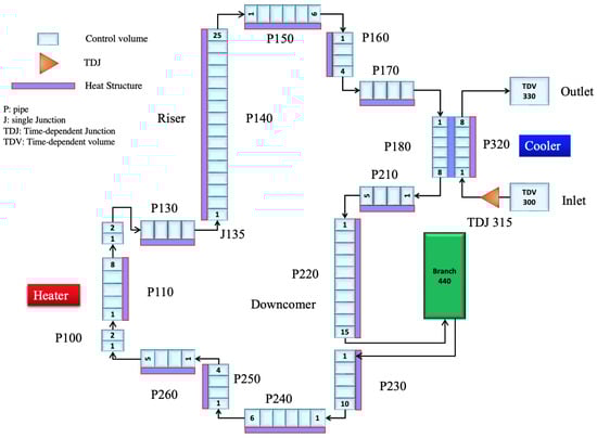
Figure 5.
RELAP5 nodalization diagram of the NC loop model.
Table 3.
Dimensions of different components in the nodalization diagram.
4.3. Model Simplifications and Sensitivity Analysis
For the RELAP5 model of the present NCL, we performed sensitivity studies to assess the impact of axial nodalization and time-step control on solution quality and cost. Axial node lengths of 6, 8, and 10 cm were tested in both the heater and cooler. The results showed a negligible impact, due to the consideration of numerical stability. On this basis, we adopted 6 cm as an accuracy–cost compromise. For numerical stability in the 1D STH discretization (RELAP5), we impose so that each control volume spans at least one hydraulic diameter; cells with display quasi-2D behavior, weaken pressure–velocity coupling, and can trigger spurious oscillations or excessive numerical diffusion. Time step and mesh size are coupled: larger axial cells reduce computational cost but tighten spatial truncation-error control, whereas smaller cells improve resolution yet reduce the allowable time step for stability. We limit the transport Courant number by enforcing
with RELAP5’s automatic controller further reducing locally if limits are violated preventing (volume skipping) and non-physical transients. The heat-exchanger (HX) region exhibits the steepest thermal–hydraulic gradients and thus dominates truncation error. For the present analysis, we introduced the following simplifications which were acknowledged as sources of model-form uncertainty:
- The two U-shaped heater elements were represented as four straight cylindrical rods.
- The HX irregular bundle was idealized as a regular triangular array.
- Total power was applied exclusively to the immersed heater; the guard-ring heater was not modeled as an active heat source.
4.4. Heat Losses Correlations
Heat losses in the NCL mostly occur through conduction and convection, as heat is transferred from the piping to the environment. These heat losses are driven by temperature gradients between the loop and its surroundings. As discussed earlier, the loop consists of both horizontal and vertical pipes which need proper heat transfer correlations in order to estimate the heat losses through each component. It is important to note that most experimental correlations estimate the average Nusselt number (Nu) for cylinders or plates under the assumption of an isothermal surface. In the present study, the methodology for determining the average Nu, and consequently the heat transfer coefficient, is illustrated in Figure 6.
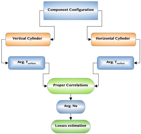
Figure 6.
A schematic diagram of heat losses estimation procedure.
Natural convection heat transfer is a widely studied topic. Numerous references offer criteria for estimating heat transfer from surfaces with various orientations, particularly for vertical cylinders and plates [34,35,36,37,38,39,40]. The Nusselt (Nu) and Grashof (Gr) numbers for vertical surfaces are determined using the height of the surface (L) as the characteristic dimension. If the boundary-layer thickness () is small relative to the diameter of the cylinder (D), the heat transfer can be calculated using the same relations applicable to vertical plates. The general criterion for treating a vertical cylinder as a vertical flat plate [41] is satisfied when
More complex correlations have been developed by Churchill and Chu [42], which are applicable over a broader range of Rayleigh numbers (Ra) for both vertical and horizontal cylinders/plates. The heat losses due to natural convection from vertical cylinders [42] (small curvature effect) and horizontal cylinders [43] are predicted using correlations in Equations (21) and (22), respectively.
For the present analysis, Equation (22) is applied to all horizontal cylinders/pipes, while Equation (21) is generally applicable to vertical cylinders with 5% error. In addition to its prior use in SPNCL studies, we adopted the Churchill–Chu correlations because (i) they match our external geometries (vertical and horizontal cylinders), (ii) they provide single, all-range expressions that remain valid from laminar through turbulent regimes and are widely recommended, and (iii) they avoid the discontinuities and regime hand-offs inherent to piecewise relations. However, for high precision with vertical cylinders, if the criteria outlined in Equation (20) are not met, Morgan [44] and Carne [45] correlations are used for the appropriate range of Ra along the surface of the isothermal cylinder. The Carne correlation is based on experimental data obtained for heated cylinders in air, applicable to a diameter range of cm and an aspect ratio range of . The average Nu number can then be estimated using Equations (23) and (24) for the Morgan and Equations (25) and (26) for the Carne correlation, respectively.
4.5. Experimental Test Matrix
The experimental matrix is divided into three primary phases: Phase 1 involves gas tests, Phase 2 focuses on water tests, and Phase 3 employs the surrogate molten salt heat transfer fluid (Therminol-66). This study focuses on the different water tests, while Phase 3’s experimental tests are still in progress. A schematic view of the experimental test matrix is shown in Figure 7, which was used to validate the system code. Furthermore, Table 4 and Table 5 provide detailed information on the various test runs using water as the working fluid, covering both steady-state and transient tests at various operating conditions. They include the initial and boundary conditions for each test. For the steady-state tests, a total of six tests were conducted: two tests at heater powers of 400 W and 800 W with a cooling water mass flow rate of 0.063 kg/s (1 gallon per minute (GPM)) and four more steady-state tests at different heater power levels of 600 W, 1000 W, 2000 W, and 3000 W with a cooling mass flow rate of 0.126 kg/s (2 GPM). The transient conditions tested included a loss of heat sink (LOHS) following the steady state and step power changes. It should be noted that the power step transients include two distinct tests. The first consists of power steps from 800 to 900 W with a 2 °C reduction in cooling water inlet temperature at a flow rate of 1 GPM. The second one involves three power steps between 1000 and 3000 W, conducted at an increased cooling water flow rate of 2 GPM to accommodate higher heat removal requirements. The present analysis reported the results related to the latter power step test.
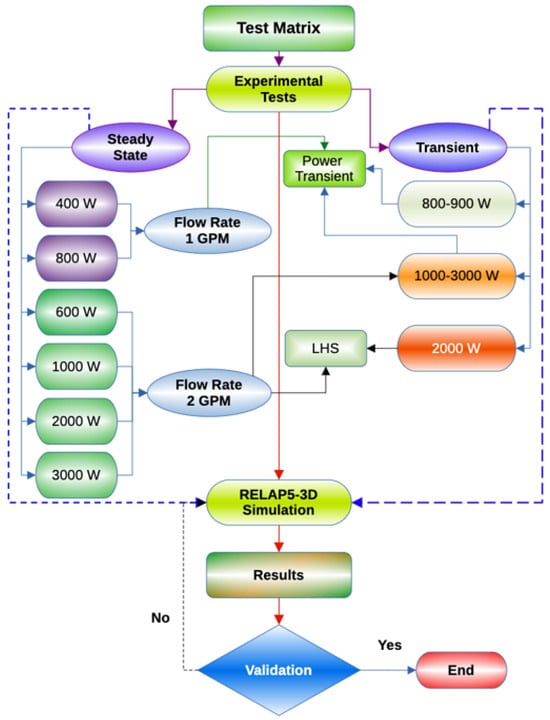
Figure 7.
Schematic view of the experimental and numerical test matrix.
Table 4.
Steady-state test matrix and BCs.
Table 5.
Transients test matrix and BCs.
5. Results and Discussion
This section presents the results obtained from system code simulations and experimental data for various steady-state and transient conditions, as outlined in Table 3 and Table 4. The aim is to assess the behavior of the natural circulation loop as well as validate the RELAP5-3D code. To evaluate the predictive capability of the model against experimental measurements, several statistical error metrics were employed. The coefficient of determination () assesses how well the model captures the overall experimental trend. The mean absolute error (MAE) quantifies the average magnitude of deviations in physical units, while the mean absolute percentage error (MAPE) provides a normalized, dimensionless measure for cross-variable comparison. The mean bias error (MBE) indicates whether RELAP5-3D model systematically overpredicts or underpredicts the experimental data. Collectively, these metrics offer a robust and transparent framework to assess model accuracy, identify systematic biases, and build confidence in the simulation results. The statistical performance metrics, including , MAE, MAPE, and MBE, together with the relative percentage error (RPE), are formally defined in Equations (27)–(31).
where N is the number of data points, is the experimental value, is the predicted value from the RELAP5-3D model, is the mean of the experimental values, and i is the data index.
5.1. Startup and Steady State Analysis
Various steady-state conditions for NC have been established at different heater power levels. Figure 8 shows the temperature profile across the heater as obtained from the RELAP5-3D code and experimental data at a heater power of 1000 W and a cooling mass flow rate of 0.126 kg/s. At the beginning of the NC transient, the sudden imbalance between heat input and the initial fluid motion leads to the appearance of these peaks. When power is first applied, the heater wall temperature rises quickly, but the fluid in contact with it is still relatively stagnant. This creates a rapid local temperature gradient and strong buoyancy forces, which momentarily accelerate the flow and drive an overshoot in outlet temperature. As circulation strengthens, cooler fluid from the inlet mixes with the hot region, reducing the gradient and damping the peak. In RELAP5, where all the thermal power is deposited directly in the immersed heater, this effect is amplified because the fluid receives the full input power instantly, leading to sharper peaks. In the experiment, part of the power goes to the guard rings and structural heat capacity, so the heating is distributed and the peaks are less pronounced. It can be noted that the code properly captured the NC phenomenon across the loop, although it reached a steady state slightly faster than the experiment, likely due to the code and experimental limitations discussed below. Figure 9 presents the temperature difference across both the heater and the cooler, with maximum deviations of 8% and 5%, respectively. Additionally, the loop mass flow rate, as predicted by the code and observed by the experimental data, is shown in Figure 10, with flow rates of approximately 0.029 and 0.031 kg/s, respectively.
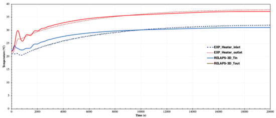
Figure 8.
Heater inlet and outlet temperature and its comparison with RELAP5-3D code at 1000 W.
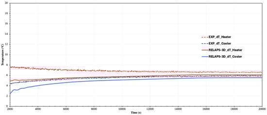
Figure 9.
Temperature difference across the heater and cooler for RELAP5-3D and experiment at 1000 W.
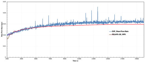
Figure 10.
Loop mass flow rate at 1000 W.
The steady-state behavior of the NCL under different heater power levels, with water as the working fluid, is illustrated in Figure 11. This figure presents a comparison between the inlet and outlet temperatures at both the heater and cooler, across different power levels, as predicted by RELAP5-3D and as observed in experimental data. It can be observed that there is a linear relationship between the system parameters (e.g., heater and cooler inlet and outlet temperatures and mass flow rate) and heating power for all pressure conditions considered, which is consistent with theoretical expectations. Furthermore, the temperature differences between the inlet and outlet of the heater which provide the primary driving head for the system are greater than those observed in the cooler under all heating powers and pressures. Also, the loop flow rates increase linearly with rising heater power, as shown in Figure 12.
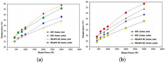
Figure 11.
Steady-state temperature validation results for the NC loop at various power levels across the heater (a) and cooler (b).
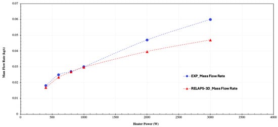
Figure 12.
Steady-state mass flow rate validation results at various power levels.
For the loop mass flow rate and temperature across the heater and cooler, it is observed that for a heater power up to 1 kW, the deviations between code predictions and experimental data are minimal. However, as heater power increases, the code tends to underestimate both the temperature and mass flow rate in the NCL. These discrepancies may arise from different sources which amplify differences, while the code increasingly underestimates both the temperatures and the mass flow. First, the test loop’s thin insulation layer causes external losses to grow rapidly with power, so the model carries too much heat away, depressing the mean loop temperature and yielding cooler ports. Second, with no primary flowmeter, the experimental is inferred from the energy balance; as power rises, larger external losses and port-zone mixing decrease the measured , biasing the inferred upwards and widening the apparent gap. Third, the RELAP5-3D model assigns all thermal power to the immersed heater, while, in the experiment, power is split between the immersed section and the guard heater/structures. The simplification in power distribution may increase the heat delivered to the fluid; consequently, the model inflates the rise in heater-side enthalpy () and the buoyancy driving head, misrepresenting the component inlet/outlet (port) temperatures and the loop mass flow (). Combined with the geometric simplifications, these factors make the 1D deck overly resistive at high temperatures, further underpredicting circulation and explaining why discrepancies grow with heater power and why the code trends low in both. Table 6 and Table 7 summarize the relative errors between the code predictions and experimental data under the specified conditions for heater and cooler temperature and loop mass flow rate, respectively.
Table 6.
Comparison of RELAP5 and experimental temperature difference across the heater and cooler at different power levels.
Table 7.
Comparison of experimental and RELAP5 mass flow rates at different heater power levels.
For the selected tests for RELAP5-3D simulation, the statistical error metrics presented in Figure 13 provide a quantitative assessment of the agreement between experimental measurements and RELAP5-3D simulation results. The grouped bar chart (left) compares four global performance indicators—mean bias error (MBE), mean absolute error (MAE), mean absolute percentage error (MAPE), and the coefficient of determination () for the three principal output parameters, namely mass flow rate, heater temperature rise, and cooler temperature drop. The MBE values are very small ( for mass flow, °C for heater for heater , and °C for heater for cooler ), indicating minimal systematic bias between RELAP5-3D and experiment. The MAE values remain below 1 unit in all cases ( for mass flow, °C for heater , and °C for heater for cooler ), while the MAPE values are modest (8.56% for mass flow, 8.43% for heater , and 9.49% for cooler ), confirming that deviations are small in both absolute and relative terms. Furthermore, the consistently high values (0.82 for mass flow, 0.92 for heater , and 0.87 for cooler ) demonstrate that the RELAP5-3D model reasonably captures the experimental trends across the tested power range.
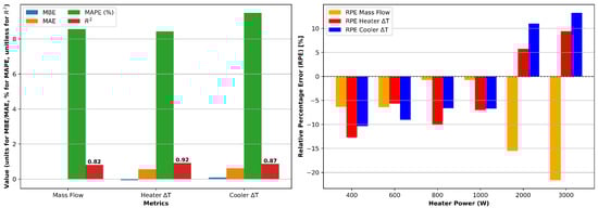
Figure 13.
Validation metrics for RELAP5 predictions against experimental data. (Left) Grouped bar chart of mean bias error (MBE), mean absolute error (MAE), mean absolute percentage error (MAPE), and . (Right) Relative percentage error (RPE) as a function of heater power.
The right panel shows the relative percentage error (RPE) given by Equation (31) as a grouped bar plot at each power level for the three key variables. Positive values indicate overprediction by the model, while negative values indicate underprediction. For the mass flow rate, the model underpredicts consistently, with errors increasing in magnitude from about at 400 W to nearly at 3000 W. This systematic underestimation reflects not only limitations in how frictional losses, local resistances, and distributed heat losses are represented in the model, but also uncertainties in the experimental loop arising from the absence of a dedicated flowmeter. Regarding heater and cooler temperature differences, the model tends to underpredict these values at lower power levels (below 2000 W), with errors ranging from at 400 W to around at 1000 W. At higher powers, however, it progressively overpredicts these values, reaching approximately for heater and for cooler at 3000 W. This crossover behavior indicates a sensitivity of the thermal–hydraulic correlations used in RELAP5-3D to the operating regime, which may be influenced by nonlinearities in natural circulation, increased heat losses at high power, and the distribution of power between the immersed heater and guard heater. Nonetheless, most RPE values remain within up to 2000 W, indicating stable predictive capability across the operating window.
5.2. Analysis of Transient Scenarios
To observe the behavior of the NCL under different transient conditions, analyses were conducted to simulate postulated accident scenarios, including the loss of heat sink, power transients, and step power changes.
5.2.1. Loss of Heat Sink (LOHS)
A loss of heat sink (LOHS) transient refers to the event in which a heat sink designed to dissipate heat fails to effectively remove heat from the system. This failure leads to a rapid increase in temperature due to the inability to transfer heat away from the heat source, often resulting in potential component damage or system failure. Such transients are critical considerations in the safety analysis of all heat transport systems, as their consequences can be severe. Consequently, most safety analyses must ensure accurate predictions. Therefore, the data presented for this type of transient is essential for effective code validation.
A steady state was established for the 2000 W test condition. Once a steady state was achieved, the secondary flow in the cooler was completely stopped at time t = 23,105 s for 1.5 h then the secondary fluid flow was restored. This termination of secondary-side water flow diminished the dissipation of heat from the water, resulting in a disturbance of the steady state and a subsequent rise in loop temperature. As shown in Figure 14, the fluid temperature at the heater inlet and outlet began to increase immediately after the secondary flow was stopped. Experimental observations indicated a significant reduction in the temperature difference between the cooler inlet and outlet during the transient, as shown in Figure 15. With the cooler no longer effectively removing heat, an average temperature difference of approximately 1.2 °C was recorded across the cooler. This reduction may be due to heat absorption by the cooler structure during the transient, resulting in some heat loss from the cooler even after secondary-side water flow was fully stopped. Meanwhile, the RELAP5-3D predicted a higher temperature difference across the cooler than was observed experimentally during the LOHS transient, while the temperature difference across the heater was predicted well by the code. This discrepancy may be attributed to temperature-dependent heat losses, which generally increase at higher loop temperatures. Additionally, in RELAP5, once the flow stops, the fluid remains stationary within the loop, allowing continued heat exchange to occur.
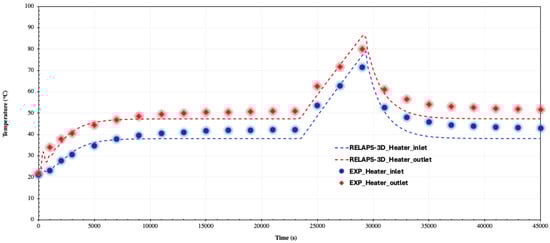
Figure 14.
Heater temperature behavior during LOHS transient at 2000 W.
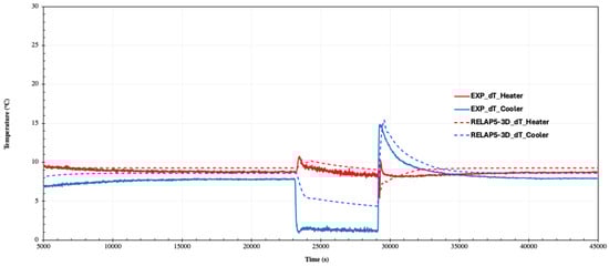
Figure 15.
Temperature difference across the heater and cooler during the LOHS transient.
5.2.2. Power Step Transient
A step power change transient is crucial for observing the system response to rapid power shifts, such as a sudden increase in turbine load, which subsequently alters reactor power. Additionally, in solar power systems, solar rays are concentrated onto the receiver using heliostats, enabling efficient energy capture [46]. In this study, a step increase in power transient was initiated by raising the main heater power from a steady-state condition of 1000 W to 3000 W, while maintaining the secondary-side water flow rate at a constant initial value of 0.126 kg/s. This increase was performed in steps: first by doubling the power to 2000 W, and subsequently increasing it to three times the initial 1000 W in the third step. The impact of this stepped power increase on the main heater is illustrated in Figure 16, showing the corresponding temperature changes. It can be observed that as the power increased from 1000 W to 2000 W and subsequently to 3000 W, the heater inlet and outlet temperatures responded accordingly, rising to reach new steady-state values with each increase in power level. From a quantitative perspective, as shown in Figure 16, the heater inlet temperature rose from an initial steady-state value of 32 °C to approximately 43 °C during the 2000 W step increase, and further to 48.33 °C during the 3000 W transient. Similarly, the heater outlet temperature shifted from 38.79 °C to 51.67 °C during the 2000 W step and reached 58.99 °C during the 3000 W step. Figure 17 presents a comparison between the temperature difference across the heater as predicted by the RELAP5-3D code and the experimental data during the step power transient. The results indicate that the RELAP5-3D code predictions are in good agreement with the experimental data, showing a 9.6% underestimation at 1000 W and overestimation of 6.1% and 9.3% during the 2000 W and 3000 W steps, respectively.
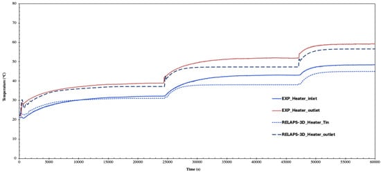
Figure 16.
Heater temperature profile following the step power transient from 1000 to 3000 W.
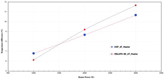
Figure 17.
Steady-state temperature difference across the heater during the step power transient for RELAP5-3D and the experiment.
6. Future Work
The present validation study with water as the working fluid has highlighted several sources of uncertainty that warrant further investigation before extending the analysis to high-viscosity surrogate fluids. First, direct measurement of the loop mass flow rate using an installed flowmeter is strongly recommended, as reliance on energy balance calculations introduces significant uncertainty, particularly under conditions of large heat losses. Second, the local hydraulic losses of the loop should be experimentally quantified rather than estimated from design data to ensure more accurate representation of pressure drop characteristics. Third, the influence of heat losses to the environment must be reduced through increase thermal insulation layer. Furthermore, analyzing the stability of the NCL is essential to establish the stability map and determine the threshold operating limits of the designed system. Finally, upgrading the test loop with a higher-power heater will expand the experimental operating window, allowing systematic investigation of natural circulation behavior under both low and high driving forces. Such an upgrade will not only strengthen the validation basis of RELAP5-3D but also provide critical insights into scaling effects and flow regime transitions that are directly relevant to advanced reactor applications.
7. Conclusions
A single-phase natural circulation loop (SPNCL) has been constructed at the University of Idaho Thermal-Hydraulics Laboratory to investigate natural circulation behavior under various operating conditions. The present analysis not only investigated the natural circulation loop (NCL) behavior with water as the working fluid but also revealed critical weaknesses in both the experimental facility and the model simplifications. Addressing these limitations will pave the way for targeted improvements in both areas, thereby ensuring that future surrogate-fluid studies dedicated to molten salt reactor (MSR) applications can be performed with greater accuracy and reduced uncertainty. As a preliminary phase, experimental studies were performed using water as the working fluid, covering both steady-state and transient conditions, including natural circulation startup, loss of heat sink (LOHS), and step changes in heater power. The RELAP5-3D system code was validated against this experimental data to assess its predictive capability.
The results demonstrate that under steady-state conditions, both loop mass flow rate and temperature rise with increasing heater power. At lower power levels (≤1000 W), the maximum deviation in mass flow rate predictions was less than 6.5%. At higher power levels of 2000 W and 3000 W, the discrepancies increased to 15.5% and 21.6%, respectively. For the temperature differences across the heater and cooler, the maximum errors remained within 13% across all operating powers. During transient tests, including LOHS and step power increases, RELAP5-3D exhibited satisfactory predictive performance, with deviations consistently below 10%.
Although the overall agreement between RELAP5-3D and experimental data is encouraging, several sources of uncertainty were identified. On the modeling side, simplifications such as applying the total thermal power exclusively to the immersed heater may have artificially enhanced buoyancy forces, contributing to flow rate discrepancies. Conversely, sensitivity analysis confirmed that tuning the heat exchanger heat transfer area had minimal influence on predictive accuracy. On the experimental side, uncertainties stem from measurement limitations, the estimation of local hydraulic losses from design data rather than direct measurements, and significant heat losses into the environment due to insufficient loop insulation. These factors are particularly important for mass flow rate predictions, emphasizing the need for direct flow measurement using a dedicated flowmeter.
Since the experimental facility provides the primary reference for RELAP5-3D code validation, it is essential to first improve the fidelity of the NCL and reduce experimental uncertainties before tuning the numerical model. Otherwise, unresolved experimental errors will propagate into the model validation process and compromise predictive reliability. The present analysis not only investigated the NCL behavior for water, but also revealed the key weaknesses of both the experimental loop and the model simplifications, thereby paving the way for targeted improvements in both areas before conducting surrogate-fluid dedicated to studying molten salt reactors (MSRs). Such refinements will help to minimize uncertainties originating from both numerical modeling and experimental measurements. In summary, RELAP5-3D demonstrated strong capabilities in reproducing natural circulation behavior under both steady-state and transient conditions, but addressing the identified uncertainties is crucial before extending this work to surrogate fluid (Therminol-66) with higher viscosity, where environmental heat losses are expected to be more pronounced.
Author Contributions
Conceptualization, H.H.A.; Methodology, H.H.A.; Data analysis, H.H.A.; Visualization, H.H.A.;Writing—original draft preparation, H.H.A.; Resources, J.Y.;Writing—review and editing, J.Y., D.A. and R.C.; Supervision, R.C. and D.A. All authors have read and agreed to the published version of the manuscript.
Funding
This research received no external funding.
Data Availability Statement
The original contributions presented in this study are included in the article. Further inquiries can be directed to the corresponding author.
Acknowledgments
This research made use of Idaho National Laboratory’s High-Performance Computing (HPC) systems located at the Collaborative Computing Center and supported by the Office of Nuclear Energy of the U.S. Department of Energy (DOE) and the Nuclear Science User Facilities (NSUF) under Contract No. DE-AC07-05ID14517.
Conflicts of Interest
Richard Christensen was employed by MicroNuclear LLC. The remaining authors declare that the research was conducted in the absence of any commercial or financial relationships that could be construed as a potential conflict of interest.
Abbreviations
The following abbreviations are used in this manuscript:
| BARC | Bhabha Atomic Research Centre |
| BC | Boundary condition |
| CFD | Computational fluid dynamics |
| CIET | Compact Integral Effects Test |
| CV | Control volume |
| CW | Cooling water |
| GFR | Gas fast reactor |
| GIF | Generation IV international forum |
| GPM | Gallon per minute |
| HPNCL | High-pressure natural circulation loop |
| HS | Heat structure |
| HX | Heat exchanger |
| INL | Idaho National Laboratory |
| LeBENC | Lead bismuth eutectic natural circulation |
| LFR | Lead fast reactor |
| LOHS | Loss of heat sink |
| MFR | Mass flow rate |
| MSBR | Molten salt breeder reactor |
| MSNCL | Molten salt natural circulation loop |
| MSR | Molten salt reactor |
| NC | Natural circulation |
| NCL | Natural circulation loop |
| ORNL | Oak Ridge National Laboratory |
| PCL | Parallel channel loop |
| PG | Pressure gauge |
| P&ID | Piping & instrumentation diagram |
| PT | Pressure transmitter |
| RELAP5 | Reactor excursion and leak analysis program |
| RTD | Resistance temperature detector |
| SAM | System analysis module |
| SCWR | Supercritical water reactor |
| SFR | Sodium fast reactor |
| SPNCL | Single-phase natural circulation loop |
| STH | System thermal hydraulics |
| TC | Thermocouple |
| TMDJ | Time-dependent junction |
| TMDV | Time-dependent volume |
| VHTR | Very-high-temperature reactor |
| VHHC | Vertical heater horizontal cooler |
| VHVC | Vertical heater vertical cooler |
Nomenclature
| A | Cross section area (m2) |
| Specific heat capacity (J/kg·K) | |
| D | Pipe diameter |
| f | Darcy friction factor |
| G | Gravitational acceleration (m/s2) |
| Grashof number | |
| H | Center to center distance between cooler and heater |
| h | Specific enthalpy (J/kg) |
| K | Loss coefficient |
| L | Length (m) |
| Mass flow rate (kg/s) | |
| Nusselt number | |
| Thermal driving head | |
| Heater electrical power (W) | |
| Frictional pressure drop | |
| Local pressure losses | |
| Resistance pressure drop | |
| Q | Heater thermal power (W) |
| Rayleigh number | |
| Reynolds number | |
| T | Temperature (°C) |
| Fluid velocity (m/s) |
Subscripts
| avg | Average |
| c | Cold |
| cl | Cold leg |
| elec | Electrical |
| f | Liquid |
| g | Vapor |
| h | Hot |
| hl | Hot leg |
| i | Inlet |
| o | Outlet |
| t | Thermal |
Greek Symbols
| Density (kg/m3) | |
| Dynamic viscosity (Pa·s) | |
| Void fraction | |
| Thermal expansion coefficient (K−1) | |
| Mass transfer | |
| Heater efficiency | |
| Boundary layer thickness (m) |
References
- GIF Portal—Portal Site Public Home. Available online: https://www.gen-4.org/gif/ (accessed on 25 July 2024).
- Weinberg, A.M. Entire volume on molten salt breeder reactor. Nucl. Appl. Technol. 1970, 8, 105. [Google Scholar]
- LeBlanc, D. Molten salt reactors: A new beginning for an old idea. Nucl. Eng. Des. 2010, 240, 1644–1656. [Google Scholar] [CrossRef]
- Rosenthal, M.W.; Kasten, P.R.; Briggs, R.B. Molten-Salt Reactors—History, Status, and Potential. Nucl. Appl. Technol. 1970, 8, 107–117. [Google Scholar] [CrossRef]
- IAEA. Status of Molten Salt Reactor Technology. Available online: https://www.iaea.org/publications/14998/status-of-molten-salt-reactor-technology (accessed on 1 August 2024).
- Serp, J.; Allibert, M.; Aumeunier, M.-H.; Baudrin, D.; Benes, O.; Delpech, S.; Ghetta, V.; Heuer, D.; Holcomb, D.; Ignatiev, V.; et al. The molten salt reactor (MSR) in Generation IV: Overview and perspectives. Prog. Nucl. Energy 2014, 77, 308–319. [Google Scholar] [CrossRef]
- Abdellatif, H.H. Experimental Validation of Single-Phase Natural Circulation Loop to Support the Development of Molten Salt Reactors. Ph.D. Thesis, University of Idaho, Moscow, ID, USA, 2025. [Google Scholar]
- Abdellatif, H.H.; Arcilesi, D.; Christensen, R.; Iskhakov, A. Similarity Analysis of High-Prandtl Surrogate Fluids for Thermal-Hydraulic Studies of Molten Salt Reactors. Ann. Nucl. Energy 2026, 225, 111757. [Google Scholar] [CrossRef]
- Welander, P. On the oscillatory instability of a differentially heated fluid loop. J. Fluid Mech. 1967, 29, 17–30. [Google Scholar] [CrossRef]
- Yun, E.; Jeon, B.-G.; Park, H.-S. Experimental study on a single-phase natural circulation loop and its steady-state solution. Appl. Therm. Eng. 2020, 173, 115190. [Google Scholar] [CrossRef]
- Abbati, Z.; Chen, J.; Cheng, K.; Zhao, F.; Tan, S. Preliminary experimental validation of multi-loop natural circulation model based on RELAP5/SCDAPSIM/MOD 4.0. Int. J. Adv. Nucl. React. Des. Technol. 2020, 2, 25–33. [Google Scholar] [CrossRef]
- Bello, S.; Gao, P.; Lin, Y. Closed-loop experimental investigation of single-phase natural circulation flow phenomena based on temperature and heating power variations. Ann. Nucl. Energy 2021, 151, 107809. [Google Scholar] [CrossRef]
- Mangal, A.; Jain, V.; Nayak, A. Capability of the RELAP5 code to simulate natural circulation behavior in test facilities. Prog. Nucl. Energy 2012, 61, 1–16. [Google Scholar] [CrossRef]
- De Vaux, R.; Aubert, P.; Grosjean, B.; Rossi, L. Flow reversals in a natural circulation loop at atmospheric pressure. Int. J. Heat Mass Transf. 2024, 235, 126119. [Google Scholar] [CrossRef]
- Vijayan, P.K. Experimental observations on the general trends of the steady state and stability behaviour of single-phase natural circulation loops. Nucl. Eng. Des. 2002, 215, 139–152. [Google Scholar] [CrossRef]
- Swapnalee, B.T.; Vijayan, P.K. A generalized flow equation for single phase natural circulation loops obeying multiple friction laws. Int. J. Heat Mass Transf. 2011, 54, 2618–2629. [Google Scholar] [CrossRef]
- Srivastava, A.K.; Saikrishna, N.; Maheshwari, N.K. Steady state performance of molten salt natural circulation loop with different orientations of heater and cooler. Appl. Therm. Eng. 2023, 218, 119318. [Google Scholar] [CrossRef]
- Vijayan, P.K.; Basak, A.; Dulera, I.V.; Vaze, K.K.; Basu, S.; Sinha, R.K. Conceptual design of Indian molten salt breeder reactor. Pramana 2015, 85, 539–554. [Google Scholar] [CrossRef]
- Srivastava, A.K.; Kudariyawar, J.Y.; Borgohain, A.; Jana, S.S.; Maheshwari, N.K.; Vijayan, P.K. Experimental and theoretical studies on the natural circulation behavior of molten salt loop. Appl. Therm. Eng. 2016, 98, 513–521. [Google Scholar] [CrossRef]
- Zweibaum, N.; Guo, Z.J.; Kendrick, J.C.; Peterson, P.A. Design of the Compact Integral Effects Test Facility and Validation of Best-Estimate Models for Fluoride Salt–Cooled High-Temperature Reactors. Nucl. Technol. 2016, 196, 641–660. [Google Scholar] [CrossRef]
- Zou, L.; Hu, G.; O’Grady, D.; Hu, R. Code validation of SAM using natural-circulation experimental data from the compact integral effects test (CIET) facility. Nucl. Eng. Des. 2021, 377, 111144. [Google Scholar] [CrossRef]
- Pilkhwal, D.S.; Ambrosini, W.; Forgione, N.; Vijayan, P.K.; Saha, D.; Ferreri, J.C. Analysis of the unstable behaviour of a single-phase natural circulation loop with one-dimensional and computational fluid-dynamic models. Ann. Nucl. Energy 2007, 34, 339–355. [Google Scholar] [CrossRef]
- Nakul, S.; Arunachala, U.C. Stability and thermal analysis of a single-phase natural circulation looped parabolic trough receiver. Sustain. Energy Technol. Assess. 2022, 52, 102242. [Google Scholar] [CrossRef]
- Zhang, T.; Brooks, C.S. Stability Tests and Analysis of a Low-Pressure Natural Circulation Loop with Flashing Instability. Nucl. Technol. 2023, 209, 1414–1441. [Google Scholar] [CrossRef]
- Sahu, M.; Sarkar, J.; Chandra, L. Effects of various modeling assumptions on steady-state and transient performances of single-phase natural circulation loop. Int. Commun. Heat Mass Transf. 2021, 124, 105247. [Google Scholar] [CrossRef]
- Abdellatif, H.H.; Young, J.; Arcilesi, D.; Christensen, R. Experimental Validation of Single-Phase Natural Circulation Loop Using Surrogate Fluid for Molten Salt Based on CFD Model to Support R&D of MSRs—Part II: Steady-State Performance of Therminol-66 as Simulant Fluid and Its Similarity Techniques Analysis. Available online: https://ssrn.com/abstract=5325163 (accessed on 11 July 2025).
- Immersion Heaters|Watlow. Available online: https://www.watlow.com/products/heaters/immersion-heaters (accessed on 23 August 2024).
- Richards, J.; Christensen, R. Design and Experimental Analysis of a Large Scale Natural Convection Test Loop. Available online: https://objects.lib.uidaho.edu/etd/pdf/Richards_idaho_0089N_11906.pdf (accessed on 18 August 2024).
- Swagelok Industrial Pressure Transducers 1067. Available online: https://www.swagelok.com/downloads/webcatalogs/en/ms-02-225.pdf (accessed on 15 July 2024).
- Stainless Steel Pressure Transducers. Available online: https://www.omega.com/en-us/pressure-measurement/pressure-transducers/p/PX309 (accessed on 10 October 2024).
- Fluke 917X Series Metrology Well Technical Guide. Available online: https://assets.testequity.com/te1/Documents/pdf/fluke/917x-tg.pdf (accessed on 12 October 2024).
- The RELAP5 Development Team. RELAP5/MOD3 Code Manual. Volume I: Code Structure, System Models and Solution Methods; NUREG/CR-5535; Idaho National Laboratory: Idaho Falls, ID, USA, 1998. [Google Scholar]
- Guillen, D.P.; Mesina, G.L.; Hykes, J.M. Restructuring RELAP5-3D for Next Generation Nuclear Plant Analysis; Transactions of the American Nuclear Society; Idaho National Lab. (INL): Idaho Falls, ID, USA, June 2006; Volume 94. [Google Scholar]
- Holman, J.P. Heat Transfer, 10th ed.; McGraw-Hill Companies Inc.: New York, NY, USA, 2010. [Google Scholar]
- Incropera, F.P. Fundamentals of Heat and Mass Transfer, 5th ed.; John Wiley & Sons: Hoboken, NJ, USA, 2009. [Google Scholar]
- Tetsu, F.; Haruo, U. Laminar natural-convective heat transfer from the outer surface of a vertical cylinder. Int. J. Heat Mass Transf. 1970, 13, 607–615. [Google Scholar] [CrossRef]
- Al-Arabi, M.; Khamis, M. Natural convection heat transfer from inclined cylinders. Int. J. Heat Mass Transf. 1982, 25, 3–15. [Google Scholar] [CrossRef]
- Cebeci, T. Laminar-Free-Convective-Heat Transfer From the Outer Surface of a Vertical Slender Circular Cylinder. In Proceedings of the 5th International Heat Transfer Conference, Tokyo, Japan, 3–7 September 1974; pp. 1–64. [Google Scholar]
- Gori, F.; Serranò, M.G.; Wang, Y. Natural Convection along a Vertical Thin Cylinder with Uniform and Constant Wall Heat Flux. Int. J. Thermophys. 2006, 27, 1527–1538. [Google Scholar] [CrossRef]
- Jarall, S.; Campo, A. Experimental Study of Natural Convection from Electrically Heated Vertical Cylinders Immersed in Air. Exp. Heat Transf. 2005, 18, 127–134. [Google Scholar] [CrossRef]
- Gebhart, B.; Jaluria, Y.; Mahajan, R.L.; Sammakia, B.; Yovanovich, M.M. Buoyancy-Induced Flows and Transport. J. Electron. Packag. 1989, 111, 321. [Google Scholar] [CrossRef]
- Churchill, S.W.; Chu, H.H.S. Correlating equations for laminar and turbulent free convection from a vertical plate. Int. J. Heat Mass Transf. 1975, 18, 1323–1329. [Google Scholar] [CrossRef]
- Churchill, S.W.; Chu, H.H.S. Correlating equations for laminar and turbulent free convection from a horizontal cylinder. Int. J. Heat Mass Transf. 1975, 18, 1049–1053. [Google Scholar] [CrossRef]
- Morgan, V.T. The Overall Convective Heat Transfer from Smooth Circular Cylinders. Adv. Heat Transf. 1975, 11, 199–264. [Google Scholar] [CrossRef]
- Carne, J.B. Heat loss by natural convection from vertical cylinders. Philos. Mag. 1937, 24, 634–653. [Google Scholar] [CrossRef]
- Sharma, A. A comprehensive study of solar power in India and World. Renew. Sustain. Energy Rev. 2011, 15, 1767–1776. [Google Scholar] [CrossRef]
Disclaimer/Publisher’s Note: The statements, opinions and data contained in all publications are solely those of the individual author(s) and contributor(s) and not of MDPI and/or the editor(s). MDPI and/or the editor(s) disclaim responsibility for any injury to people or property resulting from any ideas, methods, instructions or products referred to in the content. |
© 2025 by the authors. Licensee MDPI, Basel, Switzerland. This article is an open access article distributed under the terms and conditions of the Creative Commons Attribution (CC BY) license (https://creativecommons.org/licenses/by/4.0/).