Deterministic Data Assimilation in Thermal-Hydraulic Analysis: Application to Natural Circulation Loops

Abstract

Recent advances in high-fidelity modeling, numerical computing, and data science have spurred interest in model-data integration for nuclear reactor applications. While machine learning often prioritizes data-driven predictions, this study focuses on data assimilation (DA) to synergize physical models with measured data, aiming to enhance predictive accuracy and reduce uncertainties. We implemented deterministic DA methods—Kalman filter (KF) and three-dimensional variational (3D-VAR)—in a one-dimensional single-phase natural circulation loop and extended 3D-VAR to RELAP5, a system code for two-phase loop analysis. Unlike surrogate-based or model-reduction strategies, our approach leverages full-model propagation without relying on computationally intensive sampling. The results demonstrate that KF and 3D-VAR exhibit robustness against varied noise types, intensities, and distributions, achieving significant uncertainty reduction in state variables and parameter estimation. The framework’s adaptability is further validated under oceanic conditions, suggesting its potential to augment baseline models beyond conventional extrapolation boundaries. These findings highlight DA’s capacity to improve model calibration, safety margin quantification, and reactor field reconstruction. By integrating high-fidelity simulations with real-world data corrections, the study establishes a scalable pathway to enhance the reliability of nuclear system predictions, emphasizing DA’s role in bridging theoretical models and operational demands without compromising computational efficiency.

1. Introduction

In thermal-hydraulic analysis, using either models or observational data alone often fails to yield accurate and consistent results. To address this issue, it is necessary to develop an effective technique for integrating mechanistic models with observation, leveraging both advantages to improve the accuracy and precision of state predictions. This approach is commonly referred to as data assimilation. Data assimilation methods have evolved through several stages, including traditional assimilation algorithms, variational algorithms, filtering algorithms, and intelligent algorithms. These methods have been widely applied in numerous non-nuclear fields such as meteorological analysis [1], earth sciences [2], industrial control [3], sensor data fusion [4], economics [5], image processing [6], and computational fluid dynamics [7]. In recent years, data assimilation algorithms have also begun to be increasingly used in nuclear-related fields such as neutron physics [8], thermal-hydraulic analysis [9], and source term analysis [10].

In thermal-hydraulic analysis, three primary data assimilation frameworks are commonly utilized. The first is the BERRU-PM + PAPIRUS/STARU framework, which employs sensitivity-based deterministic methods for (approximately) linear problems and Markov Monte Carlo sampling for nonlinear problems. This framework is primarily used for uncertainty quantification [11], experimental data assimilation [12,13], and reactor design. Jaeseok Heo [9] analyzed whether the system response (i.e., sensor signals) and system attributes (e.g., DNBR) exhibit linear dependencies on parameters. A Bayesian method was employed for mildly nonlinear transients to derive the posterior distributions of parameters under the assumption of Gaussian distributions for input parameters and responses. For strongly nonlinear transient processes, a Markov chain Monte Carlo (MCMC) method based on Bayes’ theorem was utilized to estimate the posterior parameter distributions. Jaeseok Heo and Kyung Doo Kim et al. [14] compared the principles, advantages, and limitations of methodologies/software tools, including DAKOTA, MOSAIQUE, and CIRCE, and introduced a statistical data analysis toolkit, PAPIRUS, designed for model calibration, uncertainty propagation, chi-squared linearity testing, and sensitivity analysis in both linear and nonlinear problems. Dong-Hun Shin and Hae-Yong Jeong et al. [15] applied PAPIRUS to perform safety margin evaluation for loss of condenser vacuum (LOCV) scenarios. Nguyen Huu Tiep, Kyung Doo Kim et al. [16] leveraged the PAPIRUS data assimilation technique to enhance system reliability by adjusting model parameters within uncertainty bounds, thereby improving the prediction accuracy of SPACE code outputs, including cladding temperature, quench time, and steam temperature. Subsequently, Nguyen Huu Tiep, Kyung-Doo Kim, and Jaeseok Heo et al. [17] developed a novel data assimilation framework, STARU, with the primary objectives of reducing computational time and improving acceptance rates in data assimilation processes for complex systems.

The second framework combines Kalman filtering with CFD algorithms or model order reduction. Its objective is to validate the integration of experimental data and numerical models to enhance nuclear reactor analysis. Xiaoyan Yang and Hongyi Yang [18] developed a subchannel analysis data assimilation scheme based on the Ensemble Kalman filter (EnKF), capable of learning from experimental data to improve void fraction estimations by over 30%. Similar work includes the application of EnKF to two-dimensional lid-driven cavities [19], TRIGA MARK II reactors [20], SG [21], and HTR RCCS systems [22]. Carolina Introini, Antonio Cammi et al. [23] integrated a reduced-order model (POD-Galerkin method) with data-driven algorithms (Kalman filter) to create an online control system incorporating real-time experimental data feedback. C. Liu and R. Fu et al. [24] proposed an assimilation framework based on the EnKF and the DDROM model. The capabilities of the data assimilation system were demonstrated through two test cases, including the two-dimensional Burgers equation and the cylindrical flow controlled by the Navier–Stokes equations.

The third framework is mainly based on the generalized empirical interpolation method (GEIM) and the parameterized background data weakening formula (PBDW), aiming to reconstruct the system’s state from local observations or optimize sensor placement. J.-P. Argaud, B. Bouriquet et al. [25] applied GEIM to solve the sensor placement problem in nuclear reactors. Riva Stefano [26] investigated integrating model order reduction (MOR) techniques with GEIM and PBDW data assimilation methods in thermal-hydraulic systems to enable real-time temperature, pressure, and velocity field estimation. Carolina Introini and Stefano Riva et al. [27] proposed a new method based on a two-step approach to study the problem of reconstructing the overall state of a system from local observations. They [28,29] then combined the GEIM, PBDW, and indirect reconstruction (IR) to reconstruct the state from the available measurements/indirect measurements. Studies at the benchmark case (3D backward-facing step) and the DYNASTY experimental facility showed GEIM slightly superior to PBDW. Stefano Riva et al.’s recent work [30] explores the possibility of model bias correction using external data, adopting the methods of GEIM and PBDW. Antonio Cammi et al. [31] used the stable version of the GEIM based on Tikhonov regularization, TR-GEIM, and an indirect reconstruction algorithm in the cyclic fuel reactor (CFR) to determine the optimal sensor placement within the core and to evaluate the feasibility of reconstructing the quantities of interest starting only from transient sparse data of fuel temperature (possibly noisy). The results show that reconstruction is feasible for both the observable and non-observable fields, even when the parameters cannot be accurately estimated.

As mentioned above, the three data assimilation frameworks primarily enhance model predictive capability, support model development, enable accident safety analysis, optimize sensor placement, and facilitate field reconstruction in nuclear thermal-hydraulic systems. Beyond these applications, data assimilation techniques constitute fundamental enablers for constructing digital twins (DTs) to advance full lifecycle management of nuclear power plants. DTs integrate five core elements [32]: physical entities, virtual entities, twin data, services, and interconnecting links. Through their intrinsic capacity to fuse physical measurements with physics-based virtual models, data assimilation generates essential twin data while implementing key services and connectivity. This establishes the foundation for plant-wide DT capabilities spanning continuous monitoring, anomaly diagnosis, predictive maintenance, and operational prognosis—ultimately enhancing safety, reliability, and economics throughout the facility lifecycle from commissioning through decommissioning.

The current data assimilation research in the field of thermal hydraulics still has certain gaps and limitations. Current implementations of the first data assimilation framework predominantly address posterior updates of model parameters (e.g., heat transfer coefficients, discharge coefficients) while neglecting the direct adjustment of field equation variables (e.g., temperature, pressure, which are usually observable variables). The framework typically attributes the difference between the model and the true value to the uncertainty of the model parameters (usually unobserved variables and time-invariant parameters). The reliance on sensitivity matrices or extensive sampling for parameter posterior estimation constrains the real-time applicability of these methods. Sensitivity-based data assimilation methods often require manual derivation or numerical approximation of parameter-response sensitivity matrices. However, the high dimensionality of these matrices (scaling with the parameter × response dimensions) incurs significant computational costs, hindering real-time data assimilation for complex systems like two-phase natural circulation, where uncertain parameters are abundant. Sampling-based methods (e.g., MCMC, particle filtering, or ensemble Kalman filtering) also face limitations due to their reliance on extensive parallel computations, sampling inefficiencies, or particle degradation, further restricting real-time applicability in such systems. The latter two frameworks have primarily been applied to small- and medium-scale single-phase systems (e.g., numerical experiments or molten salt reactors), where governing equations and constitutive relations are simpler, and phenomenological uncertainties are lower than in two-phase systems. Observational data in such systems are also more concentrated, facilitating model reduction, surrogate modeling, or data assimilation while ensuring efficiency and accuracy for real-time applications. However, their applicability to two-phase natural circulation systems in commercial pressurized water reactors (e.g., primary/secondary loops during LOCA accidents or passive safety systems) remains understudied. These systems exhibit larger scales, greater complexity, sparser observations, and higher uncertainties (including flow instabilities), potentially leading to ill-posed governing equations. Such challenges complicate the implementation of data-driven methods and assimilation schemes relying on these frameworks. Furthermore, the assimilative capabilities of safety analysis codes, widely employed in accident simulations and plant licensing, remain inadequately evaluated. This oversight impedes the practical deployment of data assimilation in operational nuclear facilities, given the entrenched reliance on these codes for regulatory and safety-critical analyses.

To address the critical limitations of existing data assimilation methods—including real-time computational constraints, dependency on pre-trained surrogate models, compromised model interpretability/extensibility, and insufficient evaluation in complex two-phase systems—this study develops a deterministic data assimilation framework specifically designed for natural circulation systems in both single-phase and two-phase regimes. The proposed approach employs three-dimensional variational (3DVAR) and Kalman filtering methods to overcome these challenges through three key innovations: (1) By utilizing deterministic assimilation rather than sensitivity-matrix-based or sampling-based methods, it significantly reduces computational costs while maintaining real-time performance, as the required matrix dimensions scale linearly with system responses rather than parameter space. (2) The direct use of the full state transition matrix from the system model eliminates dependence on surrogate models or reduction techniques, preserving the physical interpretability and extensibility crucial for nuclear safety applications. (3) Comprehensive application to two-phase natural circulation systems, including PWR passive safety systems, addresses a significant research gap in previous studies that focused primarily on smaller single-phase systems. This framework enables robust, real-time data assimilation while maintaining compatibility with high-fidelity system analysis codes, representing an advancement for thermal-hydraulic data assimilation and safety analysis in nuclear reactors.

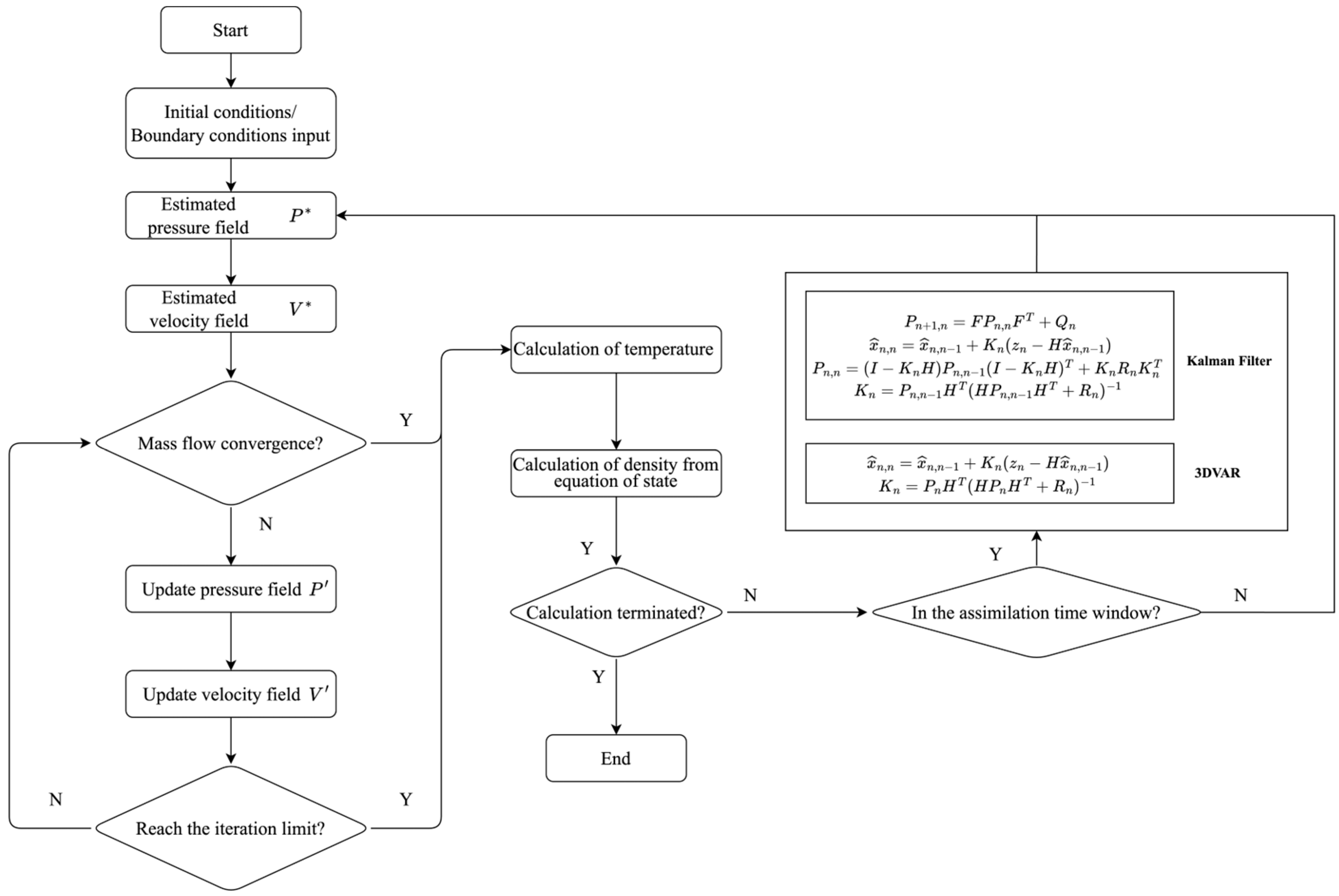
2. Deterministic Data Assimilation Methods

Data assimilation in thermal hydraulics involves three fundamental components: the base model, observations, and the assimilation technique. Current best practices indicate that one-dimensional two-phase models, despite their inherent uncertainties, are sufficiently advanced for most safety analysis requirements of thermal-hydraulic phenomena in reactors, driven by mass/heat source and sink terms. Observational data in thermal-hydraulic systems—distributed across primary/secondary loops and containment—comprise continuously sampled physical variables (e.g., temperature, pressure, water level). While these measurements offer high temporal resolution, their spatial coverage is inherently limited to discrete sensor locations. This contrasts with reactor physics measurements, which typically focus on localized regions (e.g., core instrumentation). The GEIM/PBDW methods employed in reactor physics rely on spatially concentrated observations and may not be fully suitable for thermal-hydraulic systems. Conversely, classical data assimilation techniques such as Kalman filtering and three-dimensional variational methods can effectively integrate these spatially discretized thermal-hydraulic observations to dynamically adjust model outputs, thereby reducing uncertainties in state and parameter estimations.

2.1. Kalman Filter

The Kalman filter can be used for state estimation of (nearly) linear systems. It can achieve posterior state estimation based on the model-based prior state estimates and observations. The Kalman filter [33] is based on minimizing the posterior state estimation error covariance and includes two stages: prediction and update.

In the case of the linear system, its state-space model can be written in the form of a state transition equation,

$${\widehat{\mathit{x}}}_{n+1,n}=\mathit{F}{\widehat{\mathit{x}}}_{n,n}+\mathit{G}{\mathit{u}}_n+{\mathit{w}}_n,$$

(1)

where ${\widehat{\mathit{x}}}_{n,n}$ is the estimate of the system vector at time step $n$. The estimate is made after taking measurement ${\mathit{z}}_n$at time step $n$. ${\widehat{\mathit{x}}}_{n+1,n}$ is the estimate of the future state (time step $n+1$). The estimate is made at the time step $n$. In other words, ${\widehat{\mathit{x}}}_{n+1,n}$ is a predicted state or extrapolated state. ${\mathit{u}}_n$ is a control or input variable (such as core power, pump speed). $\mathit{F}$ is a state transition matrix. $\mathit{G}$ is a control or input transition matrix (mapping control to state variables). ${\mathit{w}}_n$ is a process noise or disturbance that can be explained as an unmeasurable input that affects the state. Measurement equations link observed variables with state variables,

$${\mathit{z}}_n=\mathit{H}{\mathit{x}}_n+{\mathit{v}}_n,$$

(2)

where ${\mathit{z}}_n$ is a measurement vector (such as water level), $\mathit{H}$ is an observation matrix, ${\mathit{x}}_n$ is an actual system state, and ${\mathit{v}}_n$ is a random noise vector.

Model and observational uncertainties are typically represented in the form of covariance matrices, where estimated covariance ${\mathit{P}}_{n,n}$, process noise covariance ${\mathit{Q}}_n$, and measurement covariance ${\mathit{R}}_n$ are defined as

$${\mathit{P}}_{n,n}=E\left({\mathit{e}}_n{\mathit{e}}_n^T\right)=E\left(({\mathit{x}}_n-{\widehat{\mathit{x}}}_{n,n}){\left({\mathit{x}}_n-{\widehat{\mathit{x}}}_{n,n}\right)}^T\right),$$

(3)

$${\mathit{Q}}_n=E\left({\mathit{w}}_n{\mathit{w}}_n^T\right),$$

(4)

$${\mathit{R}}_n=E\left({\mathit{v}}_n{\mathit{v}}_n^T\right),$$

(5)

where $E$ represents the mathematical expectation and $T$ stands for transpose. Because of the unavailability of actual states, the covariance matrix is often based on prior information from statistics and is propagated using the formula

$${\mathit{P}}_{n+1,n}=\mathit{F}{\mathit{P}}_{n,n}{\mathit{F}}^T+{\mathit{Q}}_n,$$

(6)

where ${\mathit{P}}_{n+1,n}$ is the covariance matrix of the subsequent state estimation. Equation (1) and Equation (6) are used at the prediction stage. The following equations are used in the update stage:

$$\begin{array}{c}{\widehat{\mathit{x}}}_{n,n}={\widehat{\mathit{x}}}_{n,n-1}+{\mathit{K}}_n({\mathit{z}}_n-\mathit{H}{\widehat{\mathit{x}}}_{n,n-1})\end{array},$$

(7)

$$\begin{array}{c}{\mathit{P}}_{n,n}=\left(\mathit{I}-{\mathit{K}}_n\mathit{H}\right){\mathit{P}}_{n,n-1}{\left(\mathit{I}-{\mathit{K}}_n\mathit{H}\right)}^T+{\mathit{K}}_n{\mathit{R}}_n{\mathit{K}}_n^T\end{array},$$

(8)

$$\begin{array}{c}{\mathit{K}}_n={\mathit{P}}_{n,n-1}{\mathit{H}}^T{\left(\mathit{H}{\mathit{P}}_{n,n-1}{\mathit{H}}^T+{\mathit{R}}_n\right)}^{-1}\end{array},$$

(9)

where ${\mathit{K}}_n$ is the Kalman gain, ${\mathit{z}}_n$ is the measurement, and $\mathit{I}$ is the identity matrix. Kalman gain reflects the assimilation correction of observational data and the model. It should be noted that some literature uses the expression ${\mathit{P}}_{n,n}=\left(\mathit{I}-{\mathit{K}}_n\mathit{H}\right){\mathit{P}}_{n,n-1}$ to update the covariance, but due to rounding errors, minor errors in calculating the Kalman gain can lead to significant computational errors. The subtraction $\left(\mathit{I}-{\mathit{K}}_n\mathit{H}\right)$ may result in a non-symmetric matrix due to floating-point errors, which ultimately leads to numerical instability.

2.2. Three-Dimensional Variational Data Assimilation

The three-dimensional variational data assimilation (3DVAR) algorithm [34] is a data assimilation algorithm that solves the optimal solution of an analytical field parameter in three dimensions, converting the problem of solving for parameter $\mathit{x}$ to be assimilated into a problem of solving for the minimal value of the objective function $J\left(\mathit{x}\right)$. The 3D variational algorithm defines the objective function as the distance between a state vector and an observation. The state vector that minimizes this objective function is the optimal value of the state quantity. The objective function is usually defined as

$$J(\mathit{x})={\displaystyle \frac{1}{2}}(\mathit{z}-\mathit{h}(\mathit{x}){)}^T{\mathit{R}}^{-1}(\mathit{z}-\mathit{h}(\mathit{x}))+{\displaystyle \frac{1}{2}}(\mathit{x}-{\mathit{x}}_{\mathit{b}}{)}^T{\mathit{P}}^{-1}(\mathit{x}-{\mathit{x}}_{\mathit{b}}),$$

(10)

where $\mathit{z}$ is an observation vector, $\mathit{h}$ is a nonlinear mapping for observation, $\mathit{R}$ and $\mathit{P}$ are the measurement noise covariance and the model (background) covariance, respectively, and ${\mathit{x}}_{\mathit{b}}$ is the model (background) vector. The minimizer of $J\left(\mathit{x}\right)$ (i.e., the analysis) can be obtained by setting the gradient of the cost functional to zero as follows:

$$\nabla J\left(\mathit{x}\right)=-{\mathit{D}}_h^T\left({\mathit{x}}_a\right){\mathit{R}}^{-1}(\mathit{z}-\mathit{h}({\mathit{x}}_a\left)\right)+{\mathit{P}}^{-1}({\mathit{x}}_a-{\mathit{x}}_b)=0,$$

(11)

where ${\mathit{D}}_h^T$ is the transpose Jacobian matrix of the operator $\mathit{h}\left(\mathit{x}\right)$ and ${\mathit{x}}_a$ is the result of the assimilation adjustment, usually referred to as the analytical vector.

For linear case (i.e., $\mathit{h}\left(\mathit{x}\right)=\mathit{H}\mathit{x},{\mathit{D}}_h^T={\mathit{H}}^{\mathit{T}}$), ${\mathit{x}}_a$ can be derived as follows:

$${\mathit{x}}_a={\mathit{x}}_b+{\mathit{P}\mathit{H}}^T(\mathit{R}+{\mathit{H}\mathit{P}\mathit{H}}^T{)}^{-1}\left(\mathit{z}-{\mathit{H}\mathit{x}}_b\right).$$

(12)

It should be noted that the background covariance of 3DVAR usually remains unchanged compared with Kalman filter which updates the background covariance by state transition matrix continuously. Hence, it is a relatively static method. At the same time, since all terms of the cost function are evaluated simultaneously, 3DVAR can be called a stationary case.

3. Case Study of Natural Circulation Loops

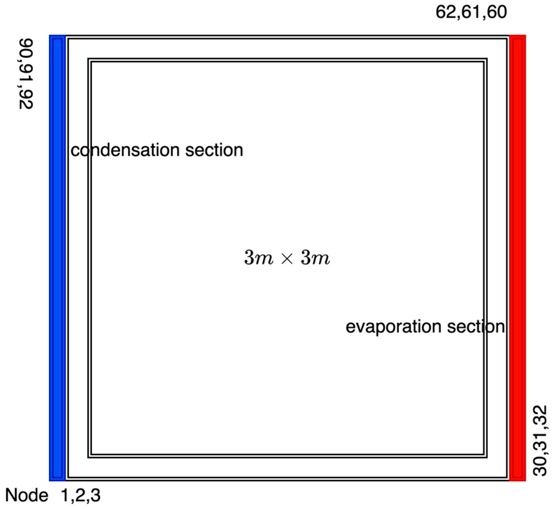
3.1. One-Dimensional Single-Phase Natural Circulation Loop

3.1.1. Model Description

A natural circulation loop serves as a fundamental component in passive system designs. Consider a square loop configuration with 3 m × 3 m dimensions, constructed using pipes with an 8 mm internal diameter. The loop consists of two primary sections: a heated zone along the right vertical segment and a condenser zone along the left vertical segment. Both zones operate under specified temperature boundary conditions that may remain constant or vary with time. This configuration is particularly suitable for integration into residual heat removal systems or emergency cooling systems of containment.

For analytical purposes, the loop structure is discretized into 120 nodes, as illustrated in Figure 1.

The single-phase natural loop control equation is as follows:

$${\displaystyle \frac{\partial \rho }{\partial t}}+{\displaystyle \frac{\partial \left(\rho u\right)}{\partial x}}=0,$$

(13)

$${\displaystyle \frac{\partial \left(\rho u\right)}{\partial t}}+{\displaystyle \frac{\partial \left(\rho uu\right)}{\partial x}}=-{\displaystyle \frac{\partial p}{\partial x}}+\rho g\mathrm{s}\mathrm{i}\mathrm{n}\theta -f{\displaystyle \frac{\Delta x}{D}}\left({\displaystyle \frac{1}{2}}\rho u^2\right),$$

(14)

$${\displaystyle \frac{\partial h}{\partial t}}={\dot{h}}_{in}-{\dot{h}}_{out}+\dot{q},$$

(15)

where $t$ stands for time, $x$ stands for distance, $\rho$ is the density, $u$ is the velocity, $p$ represents pressure, $g$ is the gravitational acceleration, $\theta$ is the vertical inclination angle (90 degrees for the ascending segment and −90 degrees for the descending segment), $f$ is the friction factor, $\Delta x$ is the length of a node, $D$ is the diameter of the pipe, $h$ represents the enthalpy, ${\dot{h}}_{in}$ and ${\dot{h}}_{out}$ are the rates of enthalpy change due to the inflow and outflow of fluid into and out of a section, respectively, and $\dot{q}$ is the wall heat transfer power.

The governing Equations (13)–(15) constitute the fundamental conservation laws for single-phase natural circulation systems. Equation (13) enforces mass conservation through continuity constraints, maintaining fluid mass balance within control volumes. Equation (14) governs momentum conservation, incorporating pressure gradients (${\displaystyle \frac{\partial p}{\partial x}}$), buoyancy forces ($\rho g\mathrm{s}\mathrm{i}\mathrm{n}\theta$), and friction losses ($f{\displaystyle \frac{\Delta x}{D}}({\displaystyle \frac{1}{2}}\rho u^2)$), thereby explicitly modeling self-sustained circulation driven by thermally induced density gradients. Equation (15) describes energy conservation via enthalpy transport and wall heat transfer power; this formulation captures essential thermal-hydraulic coupling. These first-principles equations provide physics-constrained foundations for data assimilation, ensuring strict adherence to conservation laws. Their discretized implementation enables direct integration of 3D-Var/Kalman filtering without surrogate approximations. Crucially, key uncertain parameters—particularly the friction factor $f$ in Equation (14) and the heat transfer coefficient embedded in $\dot{q}$ in Equation (15)—are implicitly targeted by our assimilation scheme to enhance robustness in complex two-phase systems.

A numerical solution program has been developed. A pressure–velocity coupling is adopted for the mass and momentum equations, and the pressure Poisson equation is solved through iteration. The pressure gradient is implicitly treated, and the convection and friction terms are explicitly treated, with the convection term using an upwind scheme and the pressure gradient using a central difference. The energy equation is based on finite differences and explicit time advancement. The program is based on the Courant condition overall and adjusts the time step based on residual convergence. The solution process is shown in Figure 2. The solver implements a projection method for incompressible natural circulation flows. Within each time step, it first computes the source term for the pressure Poisson equation (representing mass conservation residual) by discretizing the continuity equation using previous density and velocity fields, with periodic boundary conditions enforcing closed-loop behavior. The pressure field is then solved implicitly via Jacobi iteration until convergence or a maximum iteration. Subsequently, the aggregated momentum source term—incorporating discretized convection (with velocity magnitude ensuring directional correctness), buoyancy effects, and frictional losses—is explicitly evaluated. The updated velocity field is explicitly derived using the pressure gradient and source terms, followed by numerical truncation of near-zero velocities for stabilization. Finally, friction factors, heat transfer coefficient, and enthalpy (temperature and density can be calculated according to the physical properties of the fluid) are updated before advancing to the next step, completing the tightly coupled solution sequence for field variables. For the convenience of the numerical solution and easy integration with the assimilation program, a deterministic assimilation program is added after solving the variables at the current time step $n$ for the next time step $n+1$. In the deterministic program module, the presence of observations at the current moment is checked, and assimilation corrections are performed only if they lie in the assimilation time window. The program is recursive in time until the computation is terminated upon reaching a given time.

To conduct the twin experiments, we assume that the following equations calculate the friction factor used in the model (background):

$$f={\displaystyle \frac{64}{Re}},Re<2300,$$

(16)

$$f=8.0(({\displaystyle \frac{8}{Re}}{)}^{12.0}+(a+b{)}^{-1.5}{)}^{0.083},Re\ge 2300,$$

(17)

where $Re$ is the Reynolds number, $a={\left\{2.47\times \mathrm{l}\mathrm{o}\mathrm{g}\left[1.0/\left({\left(7.0/Re\right)}^{0.9}+0.27\times {10}^{-5}\right)\right]\right\}}^{16}$, and $b=(3.75\times {10}^4/Re{)}^{16}$. We assume that the true (or referred to as a reference, which is used to generate actual states and observations) expression of the coefficient of friction is

$$f={\displaystyle \frac{64}{Re}},Re<1502,$$

(18)

$$f={\displaystyle \frac{0.184}{R{e}^{0.2}}},1502\le Re\le 500000,$$

(19)

$$f=0.11\times ({10}^{-5}+{\displaystyle \frac{68}{Re}}{)}^{0.25},Re>500000.$$

(20)

The heat transfer coefficients [35] used in the model (background) calculations are

$$Nu=6.3+0.0167P{e}^{0.827}P{r}^{0.08},$$

(21)

where $Nu$ is the Nusselt number, $Pr$ is the Prandtl number (properties evaluated at fluid and wall average temperature), and $Pe$ is the Peclet number. The accurate (reference) calculation expressions of the heat transfer coefficient [36] are

$$Nu=A+0.018Pe, A=\left\{\begin{array}{c}4.5, Pe\le 1000\\ 5.4-9\times {10}^{-4}Pe,1000<Pe<2000\\ 3.6, Pe\ge 2000\end{array}\right..$$

(22)

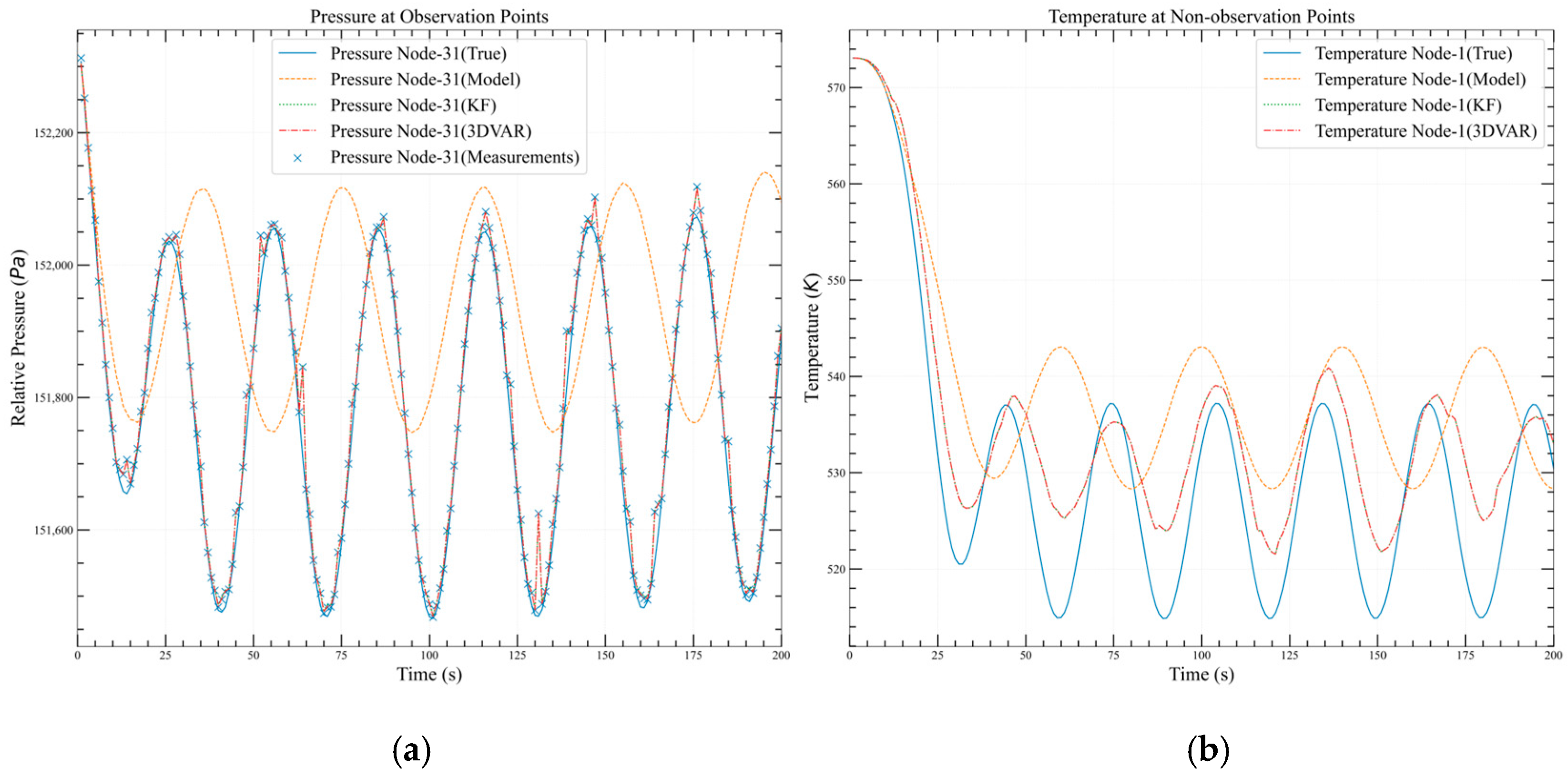
3.1.2. Fixed Wall Temperature Case

For the case where the temperature of the condensing and evaporating section is fixed, we consider that the observed data are generated by the actual state, superimposed on the Gaussian distribution noise. The frequency of the observed data is once per second; the specific observation positions are nodes 16, 31, 60, 91, 105, and 120. The observed variables are pressure, temperature, and velocity. The background covariance and measurement noise covariance matrices retain only diagonal elements representing the independence between the variables, the exact values of which can be set based on a priori information or manually adjusted by experience.

We conducted a series of numerical experiments to test the accuracy prediction ability of the assimilation algorithm under different noise levels, and the results are shown in

Table 1. Relative deviation of the baseline model, 3DVAR, and KF from the actual state under low observation noise and high observation noise. Evaporation section temperature.$T_{eva}=$ 623.16 K, condensation section temperature $T_{conden}$ = 523.16 K.

Noise	Models	Pressure	Temperature	Velocity
$\mathrm{Pressure} \mathrm{observation} \mathrm{noise} \mathrm{amplitude} A_{pressure}=5$$\mathrm{Pa}, \mathrm{observation} \mathrm{standard} \mathrm{deviation} {\sigma }_{pressure}=1$$\mathrm{Pa}. \mathrm{Temperature} \mathrm{observation} \mathrm{noise} \mathrm{amplitude} A_{temperature}=1$$\mathrm{K}, \mathrm{observation} \mathrm{standard} \mathrm{deviation} {\sigma }_{temperature}=0.5$ K	Model (Frobenius)	$1.0000$	1.0000	1.0000
	3DVAR (Frobenius)	$0.6975$	0.6298	0.6660
	KF (Frobenius)	$0.6898$	0.6298	0.6660
	Model (DTW)	$1.0000$	$1.0000$	1.0000
	3DVAR (DTW)	$0.6570$	$0.6972$	0.5894
	KF (DTW)	$0.6649$	$0.6972$	0.5895
$\mathrm{Pressure} \mathrm{observation} \mathrm{noise} \mathrm{amplitude} A_{pressure}=20$$\mathrm{Pa}, \mathrm{observation} \mathrm{standard} \mathrm{deviation} {\sigma }_{pressure}=5$$\mathrm{Pa}. \mathrm{Temperature} \mathrm{observation} \mathrm{noise} \mathrm{amplitude} A_{temperature}=5$$\mathrm{K}, \mathrm{observation} \mathrm{standard} \mathrm{deviation} {\sigma }_{temperature}=2.5$ K	Model (Frobenius)	$1.0000$	1.0000	1.0000
	3DVAR (Frobenius)	$1.2938$	0.8153	0.7329
	KF (Frobenius)	$1.3390$	0.8153	0.7334
	Model (DTW)	$1.0000$	$1.0000$	1.0000
	3DVAR (DTW)	$0.9647$	$1.2883$	0.6543
	KF (DTW)	$1.0311$	$1.2883$	0.6545

. The Frobenius norm presented in the tables represents the Difference In The state values at all the grid points over all the time steps of the computations, defined as follows:

$$L=\parallel A{\parallel }_F\equiv \sqrt{\sum _{i=1}^m\sum _{j=1}^{120}{\left|a_{ij}\right|}^2}=\sqrt{\sum _{i=1}^m\sum _{j=1}^{120}{\left|x_{ij}-{\widehat{x}}_{ij}\right|}^2},$$

(23)

where $x_{ij}$ represents the actual state (pressure, temperature, velocity, etc.) of the $j$-th node at the $i$-th moment, and ${\widehat{x}}_{ij}$ represents the estimated (model estimated or assimilation adjusted) state of the $j$-th node at the $i$-th moment. Meanwhile, the DTW (Dynamic Time Warping) distance [37] measures the temporal similarity between the predicted states and the actual values at all grid points. These two metrics can be used to assess the difference between the model or assimilation results and the actual results; the smaller the value of the metric, the closer the model/assimilation results are to the actual results, and the less uncertainty there is.

The results indicate that the 3DVAR and KF methods perform similarly under varying noise levels. Both methods can significantly enhance the accuracy of state predictions under low noise conditions. Under high noise conditions, while there is a slight reduction in pressure prediction accuracy due to substantial deviations in observation data, the temperature prediction during the ascent and descent sections and the velocity prediction still show improvements, demonstrating strong robustness. As shown in Figure 3, the Kalman filtering results closely match those of 3DVAR. Both methods exhibit comparable performance in the steady state case (t = 500 s). This is due to the fact that the Kalman filter in the steady state case can be degenerated to a three-dimensional variational one, since the state transfer matrix is a unitary matrix. The similarity between the 3DVAR assimilation predictions and the model values in this scenario arises because the deviations between the model and true state are small, while the observation noise is high. Consequently, the Kalman gain becomes sufficiently small, causing the assimilation procedure to weight the model predictions more heavily—though not exclusively—than the noisy observations. The velocity improvement at unobserved nodes in Figure 3 stems from propagated corrections originating from observed nodes. Figure 4 demonstrates pressure and temperature improvements under transient conditions. During transients, significant deviations exist between model predictions and true values. The larger background covariance yields higher Kalman gain, biasing assimilation results toward observations. Meanwhile, increased velocity-pressure iterations ensure mass convergence in transient cases. Corrections from observed nodes propagate to non-assimilated nodes, preventing substantial deviation from true values caused by excessive observation noise.

On an Intel i9-10900 CPU, for a typical single-phase natural circulation case with a problem time of 500 s, the baseline model computation time is 398 s, 3DVAR requires 430 s, and KF takes 459 s. Both the baseline model and assimilation algorithms are capable of faster-than-real-time prediction, with 3DVAR slightly outperforming KF as it avoids computing covariance update equations. Computation speed depends on numerous factors, including problem type, computational settings (convergence criteria, iteration limits, etc.), observation frequency, and noise. Therefore, appropriate configuration is essential in practical applications.

3.1.3. Time-Varying Wall Temperature Case

Consider the buoyancy-driven flow motion induced by temperature on the wall with spatial cosine and time sinusoidal variations. The following equation defines the temperatures in the evaporation ($T_{eva}$) and condensation sections ($T_{cond}$):

$$T_{eva}=T_{evainit}+A_1\mathit{cos}x+A_3\mathit{sin}2\pi t/T$$

(24)

$$T_{cond}=T_{condinit}+A_2\mathit{cos}x+A_3\mathit{sin}2\pi t/T,$$

(25)

where $t$ stands for time and $x$ represents distance. For the actual working condition, we assume that $T_{evainit}=623.16K,{T_{condinit}=523.16K,A}_1=10,A_2=15,A_3=20, \mathrm{a}\mathrm{n}\mathrm{d} T=30s$. For model calculation, $T_{evainit}=613.16K,{T_{condinit}=533.16K,A}_1=5, \mathrm{a}\mathrm{n}\mathrm{d} A_2=10,A_3=15,T=40s$. The difference between the actual state and the model reflects the measurement and cognitive uncertainty about the working conditions. The observation node locations and frequency are consistent with the previous setup. The observed variables are limited to temperature and pressure.

Table 2. Relative deviation of the baseline model, 3DVAR, and KF from the actual state under Gauss and Lognormal observation noise.

Noise	Models	Pressure	Temperature	Velocity
$\mathrm{Pressure} \mathrm{observation} \mathrm{noise} \mathrm{amplitude} A_{pressure}=10$$\mathrm{Pa}, \mathrm{observation} \mathrm{standard} \mathrm{deviation} {\sigma }_{pressure}=1$$\mathrm{Pa}. \mathrm{Temperature} \mathrm{observation} \mathrm{noise} \mathrm{amplitude} A_{temperature}=2$$\mathrm{K}, \mathrm{observation} \mathrm{standard} \mathrm{deviation} {\sigma }_{temperature}=1$ K. (Gauss)	Model (Frobenius)	$1.0000$	$1.0000$	1.0000
	3DVAR (Frobenius)	$0.9337$	$0.8323$	0.9141
	KF (Frobenius)	$0.9371$	$0.8323$	0.9141
	Model (DTW)	$1.0000$	$1.0000$	$1.0000$
	3DVAR (DTW)	$0.9764$	$0.5864$	$0.9235$
	KF (DTW)	$0.9917$	$0.5864$	$0.3295$
$\mathrm{Pressure} \mathrm{observation} \mathrm{noise} \mathrm{amplitude} A_{pressure}=10$$\mathrm{Pa}, \mathrm{observation} \mathrm{standard} \mathrm{deviation} {\sigma }_{pressure}=1$$\mathrm{Pa}. \mathrm{Temperature} \mathrm{observation} \mathrm{noise} \mathrm{amplitude} A_{temperature}=2$$\mathrm{K}, \mathrm{observation} \mathrm{standard} \mathrm{deviation} {\sigma }_{temperature}=1$ K. (Lognormal)	Model (Frobenius)	$1.0000$	$1.0000$	$1.0000$
	3DVAR (Frobenius)	$0.9337$	$0.8399$	0.9222
	KF (Frobenius)	$0.9446$	$0.8399$	0.9222
	Model (DTW)	$1.0000$	$1.0000$	$1.0000$
	3DVAR (DTW)	$0.9842$	$0.6010$	$0.9341$
	KF (DTW)	$1.0219$	$0.6010$	$0.9341$

demonstrates assimilation results under Gaussian noise and Lognormal distribution, indicating that 3DVAR and KF effectively compensate for state prediction inaccuracies under dynamic responses. Moreover, these methods exhibit robust assimilation performance, even when dealing with lognormal distribution noise. Even in the absence of speed observations, the accuracy of speed predictions has been improved due to precision corrections for temperature and pressure. At the same time, due to the non-reliance on sampling, the computational speed of the assimilation program is roughly consistent with that of the benchmark model.

Figure 5 shows the predicted temperature and velocity under quasi-steady-state conditions. The predictions from the Kalman filter and 3DVAR are very similar. Temperature predictions show significant accuracy improvements near observation points, with these improvements diminishing with increasing distance from the points, gradually converging toward the baseline model. Velocity predictions, on the other hand, remain close to the model overall, as the nodes lack direct observational information and rely on propagation from other nodes. Figure 6 demonstrates that when both model and process covariance parameters are set to larger values, the Kalman gain approaches unity, leading to assimilation results that exhibit a stronger reliance on measurements. Concurrently, due to phase discrepancies between the true states and model predictions across temporal cycles, the assimilated outputs manifest distinct time-varying characteristics while achieving smoothed transitions between observational data and modeled values. This behavior highlights the system’s adaptive balancing mechanism under high covariance configurations, where measurement trustworthiness dominates while preserving dynamical consistency through transitional smoothing.

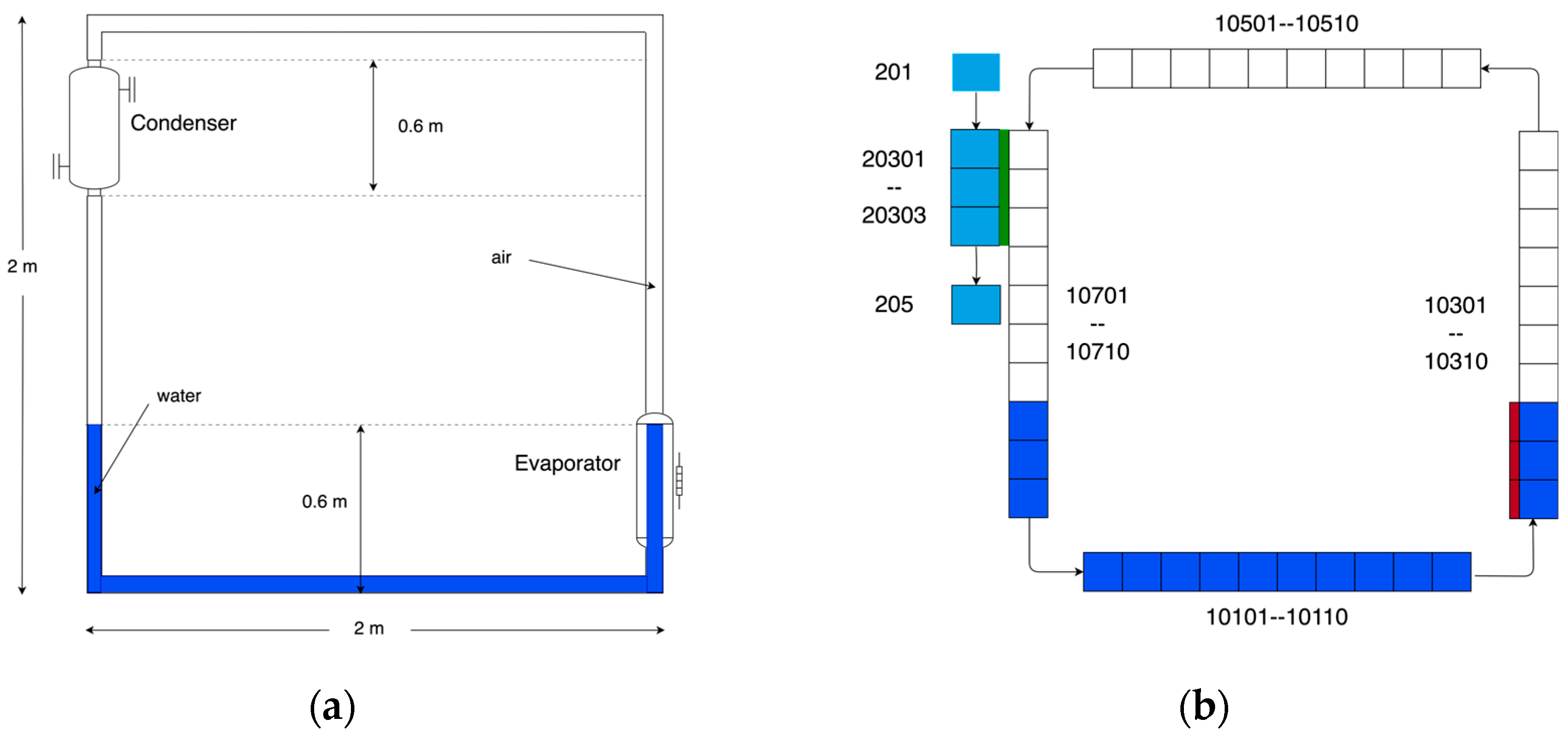
3.2. One-Dimensional Two-Phase Natural Circulation Loop

Two-phase natural circulation loops are widely employed in waste heat removal systems of nuclear reactors, particularly in pressurized water reactors, owing to their advantages, such as efficient heat transfer and structural simplicity. However, phase change introduces uncertainties and complexities, making the thermal-hydraulic analysis more challenging.

To verify the precision compensation capability of assimilation technology for two-phase natural circulation, a natural circulation loop, as depicted in Figure 7, was modeled. The loop [38] consists of four round pipes, each with a diameter of 1 cm and a length of 2 m. The lower part of the pipe is filled with liquid water, while the upper part contains air. At the bottom of the loop, an evaporation section is electrically heated with a 2000 W heat source and has a thickness of 2 mm. At the top of the loop, a cooling section uses a convective cooling jacket. This jacket features a pipe wall thickness of 2 mm and an outer diameter of 2.4 cm. The liquid water in the condensing jacket is circulated by a pump operating at a speed of 1 m/s.

The natural circulation loop was simulated through the MELCOR system code, the standard RELAP5 thermal-hydraulic code, and an enhanced RELAP5-3DVAR variant. The latter constitutes a modified RELAP5-based benchmark framework incorporating a three-dimensional variational (3DVAR) data assimilation module. The numerical procedure follows a sequential prediction-correction scheme: Following the advancement of the thermal-hydraulic solution to time step n, state variable predictions for n + 1 are generated through conventional RELAP5 calculations, subsequently refined via the variational optimization formulation described in Equation (12).

MELCOR simulation outputs served as the reference dataset (“truth system”) for assimilating RELAP5 predictions within this validation paradigm. The MELCOR code was specifically selected to provide thermal-hydraulic modeling capabilities while maintaining differences from RELAP5 in modeling resolution, field equations, solution strategies, and constitutive models. This tests the robustness of the RELAP5-3DVAR assimilation code in absorbing data from different source codes. Observational constraints comprised synchronized pressure and temperature measurements sampled at 1 Hz frequency from mid-section monitoring points. As evidenced in Figure 8, the RELAP5-3DVAR implementation demonstrates marked enhancement in predicting both the evaporative heat structure temperature profile and condensation heat transfer coefficients—improvements attributable to the framework’s enhanced fidelity in predicting critical system state variables (particularly fluid temperature and pressure fields). These enhancements persist despite the absence of direct empirical measurements, indicating successful propagation of observational information through coupled thermofluidic interactions.

3.3. One-Dimensional Two-Phase Natural Circulation Loop Under Ocean Conditions

The case above demonstrates data assimilation’s precision compensation capability for model correction. We designed a numerical case to illustrate the potential of data assimilation in model extension prediction. Consider a two-phase natural circulation loop deployed on a floating platform, where the actual state is derived from superimposed heaving and rolling motions, calculated using RELAP5 with an added ocean model [39].

The nodalization of the circulation loop is illustrated in Figure 9, with control volumes 112 and 122 representing the evaporator and 302 denoting the condenser. The loop undergoes sinusoidal heave motion along the z-axis (amplitude: 3.0 m/s², period: 10.0 s, initiated at t = 20.0 s), coupled with rotational oscillation about the (0,1,0)-aligned axis (angular amplitude: 15°, period: 15.0 s, initiated at t = 40.0 s). The rotation axis is spatially referenced to control volume 100,010,000 at coordinates (0.0,0.0,1.0), corresponding to a position 1.0 m downward along the z-axis relative to the control volume’s local coordinate system.

The baseline model calculation uses RELAP5 without the ocean model. Observation data are directly taken from the actual state, including temperature, pressure, and void fraction at specific nodes in the evaporation, condensation, and transport sections. The observation frequency is once per second. The assimilation results (Figure 10) below indicate that the RELAP5-3DVAR can enhance system state prediction without the ocean model, demonstrating a specific capability for model extension prediction. It aligns with previous single-phase and two-phase natural circulation cases. The robust performance of 3D-Var stems from its objective function design, which minimizes discrepancies between model-corrected predictions, observations, and baseline models. This approach ensures corrected predictions strike a balance between baseline models and observations.

Given the potential marine deployment of future small modular reactors, the two-phase natural circulation loops configured on floating nuclear power platforms are inevitably influenced by ocean waves, leading to fluctuations and sway. Current models often rely on assumed fluctuation accelerations and sway periods, which may not accurately reflect the sea conditions at deployment sites. This discrepancy challenges floating nuclear power plants’ safety analysis, design, and operation. The model correction and extrapolation capabilities provided by assimilation codes effectively address these discrepancies, reducing the conservatism in design imposed by uncertainties.

4. Conclusions

We have developed benchmark solvers and integrated versions with the Kalman filter and three-dimensional variational data assimilation for a one-dimensional single-phase natural circulation loop. The results demonstrate that the Kalman filter and the three-dimensional variational data assimilation are effective in making correct model predictions with minimal data for cases with fixed temperature boundaries and time-varying boundary conditions. These methods perform robustly under varying noise intensity and distributions. A three-dimensional variational assimilation code was developed based on RELAP5 for one-dimensional two-phase natural circulation loops. The results show that integrating observational data from the MELCOR and RELAP5-ocean models significantly improves state predictions, including model parameter estimation. This highlights the potential of the assimilation procedure not only for model correction but also for reliable extrapolation.

Future work will focus more on studying the experimental and plant real-time data, which will provide insight into efficiency, accuracy, and robustness.

References

1. Lorenc, A.; Bell, R.; Macpherson, B. The Meteorological Office analysis correction data assimilation scheme. Q. J. R. Meteorol. Soc. 1991, 117, 59–89. [Google Scholar] [CrossRef]
2. Carrassi, A.; Bocquet, M.; Bertino, L.; Evensen, G. Data assimilation in the geosciences: An overview of methods, issues, and perspectives. Wiley Interdiscip. Rev. Clim. Change 2018, 9, e535. [Google Scholar] [CrossRef]
3. Chenyu, J.; Jun, Y.; Ke, X.; Zhanyu, H.; Ming, Y. Coupling of adjoint-based Markov/CCMT predictive analytics with data assimilation for real-time risk scenario forecasting of industrial digital process control systems. Process Saf. Environ. Prot. 2023, 171, 951–974. [Google Scholar] [CrossRef]
4. Jahja, M.; Farrow, D.; Rosenfeld, R.; Tibshirani, R.J. Kalman filter, sensor fusion, and constrained regression: Equivalences and insights. Adv. Neural Inf. Process. Syst. 2019, 32. [Google Scholar] [CrossRef]
5. Nadler, P.; Arcucci, R.; Guo, Y.-K. Data assimilation for parameter estimation in economic modelling. In Proceedings of the 2019 15th International Conference on Signal-Image Technology & Internet-Based Systems (SITIS), Sorrento, Italy, 26–29 November 2019. [Google Scholar] [CrossRef]
6. Beyou, S.; Cuzol, A.; Gorthi, S.S.; Mémin, E. Weighted ensemble transform Kalman filter for image assimilation. Tellus A Dyn. Meteorol. Oceanogr. 2013, 65, 18803. [Google Scholar] [CrossRef]
7. Mons, V.; Chassaing, J.-C.; Gomez, T.; Sagaut, P. Reconstruction of unsteady viscous flows using data assimilation schemes. J. Comput. Phys. 2016, 316, 255–280. [Google Scholar] [CrossRef]
8. Gong, H. Data Assimilation with Reduced Basis and Noisy Measurement: Applications to Nuclear Reactor Cores. Doctoral Dissertation, Sorbonne Université, Paris, France, 2018. [Google Scholar]
9. Heo, J. Optimization of Design for SMR via Data Assimilation and Uncertainty Quantification; NC State University: Raleigh, NC, USA, 2011. [Google Scholar]
10. Li, K.; Chen, W.; Liang, M.; Zhou, J.; Wang, Y.; He, S.; Yang, J.; Yang, D.; Shen, H.; Wang, X. A simple data assimilation method to improve atmospheric dispersion based on Lagrangian puff model. Nucl. Eng. Technol. 2021, 53, 2377–2386. [Google Scholar] [CrossRef]
11. Cacuci, D.G.; Ionescu-Bujor, M. Best-Estimate Model Calibration and Prediction through Experimental Data Assimilation—I: Mathematical Framework. Nucl. Sci. Eng. 2010, 165, 18–44. [Google Scholar] [CrossRef]
12. Petruzzi, A.; Cacuci, D.G.; D’Auria, F. Best-Estimate Model Calibration and Prediction through Experimental Data Assimilation—II: Application to a Blowdown Benchmark Experiment. Nucl. Sci. Eng. 2010, 165, 45–100. [Google Scholar] [CrossRef]
13. Cacuci, D.G.; Arslan, E. Reducing Uncertainties via Predictive Modeling: FLICA4 Calibration Using BFBT Benchmarks. Nucl. Sci. Eng. 2014, 176, 339–349. [Google Scholar] [CrossRef]
14. Heo, J.; Kim, K.D. PAPIRUS, a parallel computing framework for sensitivity analysis, uncertainty propagation, and estimation of parameter distribution. Nucl. Eng. Des. 2015, 292, 237–247. [Google Scholar] [CrossRef]
15. Shin, D.-H.; Jeong, H.-Y.; Park, M.-G.; Sohn, J.-U. Application of a combined safety approach for the evaluation of safety margin during a Loss of Condenser Vacuum event. Nucl. Eng. Technol. 2022, 54, 1698–1711. [Google Scholar] [CrossRef]
16. Tiep, N.H.; Kim, K.D.; Heo, J. Improvement in the accuracy of SPACE prediction for the unblocked FLECHT SEASET reflood tests by data assimilation. Ann. Nucl. Energy 2021, 161, 108462. [Google Scholar] [CrossRef]
17. Tiep, N.H.; Kim, K.-D.; Heo, J.; Choi, C.-W.; Jeong, H.-Y. A newly proposed data assimilation framework to enhance predictions for reflood tests. Nucl. Eng. Des. 2022, 390, 111724. [Google Scholar] [CrossRef]
18. Yang, X.; Yang, H. Data Assimilation in Sub-Channel Analysis Model Based on Ensemble Kalman Filter. In Proceedings of the International Conference on Nuclear Engineering, Online, 8–12 August 2022. [Google Scholar] [CrossRef]
19. Introini, C.; Lorenzi, S.; Cammi, A.; Baroli, D.; Peters, B.; Bordas, S. A Mass Conservative Kalman Filter Algorithm for Computational Thermo-Fluid Dynamics. Materials 2018, 11, 2222. [Google Scholar] [CrossRef]
20. Introini, C.; Chiesa, D.; Lorenzi, S.; Nastasi, M.; Previtali, E.; Salvini, A.; Sisti, M.; Snoj, L.; Antonio, C. Assessment of the integrated mass conservative Kalman filter algorithm for Computational Thermo-Fluid Dynamics on the TRIGA Mark II reactor. Nucl. Eng. Des. 2021, 384, 111431. [Google Scholar] [CrossRef]
21. Fang, P.; He, C.; Wang, P.; Xu, S.; Liu, Y. Data Assimilation of Steam Flow Through a Control Valve Using Ensemble Kalman Filter. J. Fluids Eng. 2021, 143, 091201. [Google Scholar] [CrossRef]
22. Liu, S.; Zhang, H.; Wu, Y.; Lang, M.; Dong, Y.; Li, F. Improving the Accuracy of RCCS Simulator Based on Ensemble Kalman Filter Algorithm. In Proceedings of the 2024 31st International Conference on Nuclear Engineering, Prague, Czech Republic, 4–8 August 2024. [Google Scholar] [CrossRef]
23. Introini, C.; Lorenzi, S.; Cammi, A.; Baroli, D. A Reduced Order Kalman Filter for Computational Fluid-Dynamics Applications. Sci. Posters 2018. [Google Scholar] [CrossRef]
24. Liu, C.; Fu, R.; Xiao, D.; Stefanescu, R.; Sharma, P.; Zhu, C.; Sun, S.; Wang, C. EnKF data-driven reduced order assimilation system. Eng. Anal. Bound. Elem. 2022, 139, 46–55. [Google Scholar] [CrossRef]
25. Argaud, J.-P.; Bouriquet, B.; De Caso, F.; Gong, H.; Maday, Y.; Mula, O. Sensor placement in nuclear reactors based on the generalized empirical interpolation method. J. Comput. Phys. 2018, 363, 354–370. [Google Scholar] [CrossRef]
26. Riva, S. Reduced Basis Methods for Data Assimilation in Real Thermal Hydraulics Systems; Polytechnic University of Milan: Milan, Italy, 2020. [Google Scholar]
27. Introini, C.; Riva, S.; Lorenzi, S.; Cavalleri, S.; Cammi, A. Non-intrusive system state reconstruction from indirect measurements: A novel approach based on Hybrid Data Assimilation methods. Ann. Nucl. Energy 2023, 182, 109538. [Google Scholar] [CrossRef]
28. Riva, S.; Introini, C.; Lorenzi, S.; Cammi, A. Hybrid data assimilation methods, Part I: Numerical comparison between GEIM and PBDW. Ann. Nucl. Energy 2023, 190, 109864. [Google Scholar] [CrossRef]
29. Riva, S.; Introini, C.; Lorenzi, S.; Cammi, A. Hybrid Data Assimilation methods, Part II: Application to the DYNASTY experimental facility. Ann. Nucl. Energy 2023, 190, 109863. [Google Scholar] [CrossRef]
30. Riva, S.; Introini, C.; Cammi, A. Multi-physics model bias correction with data-driven reduced order techniques: Application to nuclear case studies. Appl. Math. Model. 2024, 135, 243–268. [Google Scholar] [CrossRef]
31. Cammi, A.; Riva, S.; Introini, C.; Loi, L.; Padovani, E. Data-driven model order reduction for sensor positioning and indirect reconstruction with noisy data: Application to a Circulating Fuel Reactor. Nucl. Eng. Des. 2024, 421, 113105. [Google Scholar] [CrossRef]
32. Tao, F.; Zhang, M.; Liu, Y.; Nee, A.Y.C. Digital twin driven prognostics and health management for complex equipment. CIRP Ann. 2018, 67, 169–172. [Google Scholar] [CrossRef]
33. Becker, A. Kalman Filter from the Ground Up. KilmanFilter.NET. 2023. Available online: https://www.kalmanfilter.net (accessed on 6 May 2025).
34. Ahmed, S.E.; Pawar, S.; San, O. PyDA: A Hands-On Introduction to Dynamical Data Assimilation with Python. Fluids 2020, 5, 225. [Google Scholar] [CrossRef]
35. Sleicher, C.A.; Awad, A.S.; Notter, R.H. Temperature and eddy diffusivity profiles in NaK. Int. J. Heat Mass Transf. 1973, 16, 1565–1575. [Google Scholar] [CrossRef]
36. Cheng, X.; Tak, N.-I. Investigation on turbulent heat transfer to lead–bismuth eutectic flows in circular tubes for nuclear applications. Nucl. Eng. Des. 2006, 236, 385–393. [Google Scholar] [CrossRef]
37. Giorgino, T. Computing and Visualizing Dynamic Time Warping Alignments in R: The dtw Package. J. Stat. Softw. 2009, 31, 1–24. [Google Scholar] [CrossRef]
38. Gong, L.; Peng, C. Analysis of the heat-carrying performance of natural circulation loop using modified RELAP5/MOD3.4. Case Stud. Therm. Eng. 2022, 39, 102387. [Google Scholar] [CrossRef]
39. Bai, T.-Z.; Peng, C.-H. Thermal hydraulic characteristics of helical coil once-through steam generator under ocean conditions. Nucl. Sci. Tech. 2022, 33, 134. [Google Scholar] [CrossRef]
Figure 1. Diagram of a single-phase natural circulation loop. (The red area represents the evaporation section, and the blue area represents the condensation section).
Jne 06 00023 g001
Figure 2. Flow chart of single-phase natural circulation loop analysis program. (* represents the estimated values of pressure and velocity).
Jne 06 00023 g002
Figure 3. State assimilation results under high measurement noise (fixed wall temperature case). The figure shows (a) temperature distribution of the tube wall at t = 500 s and (b) velocity versus time curve for non-observed points.
Jne 06 00023 g003
Figure 4. State assimilation results under high measurement noise (fixed wall temperature case). Comparison of (a) pressure and (b) temperature changes over time under real, model, and assimilation programs. Measurements are based on real data with noise added.
Jne 06 00023 g004
Figure 5. State assimilation results under high measurement noise (time-varying wall temperature case). The figure shows (a) temperature distribution of the tube wall at t = 500 s and (b) velocity versus time curve for non-observed points.
Jne 06 00023 g005
Figure 6. State assimilation under log-normal distribution observation noise with time-varying boundary conditions. Comparison of (a) pressure and (b) temperature changes over time under real, model, and assimilation programs. Measurements are based on real data with noise added.
Jne 06 00023 g006
Figure 7. (a) Schematic of a two-phase natural circulation loop; (b) RELAP5 modeling node diagram. (Blue represents water, red represents the heating section, and green represents the condensation section).
Jne 06 00023 g007
Figure 8. Two-phase natural circulation loop state prediction and parameter estimation based on 3DVAR. The figure shows (a) the assimilation result of evaporator temperature and (b) the condenser heat transfer coefficient.
Jne 06 00023 g008
Figure 9. RELAP5 nodalization of a two-phase natural circulation loop deployed on a floating platform.
Jne 06 00023 g009
Figure 10. 3DVAR-based prediction of the state of a two-phase natural circulation loop under oceanic conditions. The figure shows (a) the assimilation results of the evaporator pressure and (b) the temperature assimilation results.
Jne 06 00023 g010