Hydrogen Production Using PVs with MPPT Optimization

Abstract

This article examines hydrogen production using Proton Exchange Membrane Electrolyzers (PEMELs) and photovoltaic (PV) panels using Maximum Power Point Tracking (MPPT). This method has great potential to maximize the production of pure hydrogen, making it possible to reduce and potentially eliminate the difficulties associated with sudden drops and interruptions in output power. The use of MPPT algorithms in conjunction with Direct Current to Direct Current (DC/DC) converters helps improve the energy efficiency of systems. This study aims to enhance green hydrogen production by optimizing PV-PEMEL performance using commercial power electronics, while improving energy storage and reducing costs for sustainable hydrogen generation.

1. Introduction

Recent advances in the utilization of PV panels and PEMELs for hydrogen generation have garnered significant academic interest due to their potential to enhance sustainable energy output. This method leverages solar energy as a renewable source to power water electrolysis, producing hydrogen and oxygen in an environmentally friendly manner. PEMELs are becoming a highly promising option for renewable hydrogen generation due to their ability to operate efficiently under variable loads. This characteristic is particularly beneficial for direct coupling with intermittent renewable energy sources like PV systems. Control strategies are essential to balance the input from PVs with the internal electrochemical processes in the electrolyzers, thereby optimizing hydrogen production.

The integration of PV systems with PEMELs presents several key technological challenges and research objectives. The development of MPPT algorithms is crucial in this field, as they ensure that PV panels operate optimally under varying irradiance and temperature conditions. Furthermore, improving energy conversion efficiency within the coupled system and developing advanced control strategies are essential for maximizing hydrogen production rates.

1.1. System Integration

The intermittency of solar energy leads to fluctuating power supplies, which diminishes the efficacy of electrolysis. Some studies recommend mitigating this instability with advanced power electronics or energy storage technologies. Conversely, direct coupling of PV modules to PEM electrolyzers is feasible only if their current–voltage characteristic curves match. Hirokazu et al. [1] also stated that direct connection was possible, but it resulted in variable hydrogen production rates due to changing solar irradiation.

Fluctuations in solar power could be stabilized using power conditioning devices, such as DC/DC converters, which optimize input power to the electrolyzer for high efficiency [2].

Efficiency values for PEM electrolyzers typically range from 60% to 70%. Further improvements are possible through advancements in membrane materials and catalysts, as noted by Ayers et al. [3]. The efficiency of PV panels directly impacts the amount of electricity available for the electrolysis process. State-of-the-art silicon-based PV cells can achieve efficiencies of 20% to 25%, and emerging perovskite or tandem cell technologies could potentially drive this above 30% [4].

PV-PEMELs face a major challenge: the periodicity of solar energy. Current integration efforts aim at developing integrated hydrogen storage solutions, whereby excess hydrogen produced during peak solar hours can be stored and subsequently used when solar radiation is unavailable. Many researchers also advocate hybrid systems that combine PVs with other renewable sources, such as wind or biomass, to smooth out the energy input to the electrolyzer. Alternatively, batteries can be used. Nevertheless, the most significant step towards mass commercialization is cost reduction. While the costs of PV panels have dropped significantly over the past 10 years, the costs of electrolyzers remain very high. Long-term studies are investigating economies of scale and cost-reduction strategies [4,5,6].

1.2. Photovoltaic Operating Point Optimization Using MPPT

PV panels are inherently nonlinear devices, with their power output dependent on both temperature and irradiance. MPPT algorithms are employed to track the maximum power as environmental conditions fluctuate. These algorithms are crucial for optimizing power transfer from the PV system to the electrolyzer, thereby maximizing hydrogen production. Among the various MPPT algorithms, Perturb and Observe (P&O), incremental Conductance (IC), fuzzy logic, neural network techniques, and particle swarm optimization are notable examples. These methods continuously adjust the operating voltage or current to track the maximum power point.

A comparative survey by Devarakonda et al. [7] has provided insights into various MPPT algorithms used to maintain optimal output power. The authors highlighted that those conventional methods, such as P&O and IC, are simple and cost-effective, whereas advanced methods like particle swarm optimization (PSO) and genetic algorithms demonstrate superior performance under rapid irradiance changes, leading to increased hydrogen yield. Kang et al. [8] also discussed adaptive MPPT strategies for dynamic solar conditions, which could be particularly effective in decentralized hydrogen production using PEMELs.

1.3. Energy Efficiency and Power Management

For effective hydrogen production, it is not only important to track the maximum power point but also to deliver optimized power to the PEMELs. In general, the overall efficiency of the system depends on efficiently transferring energy from the PV array to the electrolyzer. Direct coupling of the PV systems and low-pressure PEMELs represents a simple and low-cost solution, but does not operate at the optimal efficiency of an electrolyzer.

The need to match the characteristics of the PV output to the power input requirements of the electrolyzer has led to research into power electronics-based interfacing systems, including DC/DC converters. Clarke et al. [9], in their work, explored direct coupling versus converter-based approaches for hydrogen production. They also proved that power electronic interfacing enhances the overall system efficiency due to the fact that an electrolyzer works closer to its ideal voltage under variable solar input conditions.

In one of their works, Dahbi et al. [10] showed the usage of DC/DC converters to optimize the input voltage to an electrolyzer for its most efficient operation. The authors believed that such converters, combined with advanced MPPT, can yield an efficiency gain of as much as 15 to 20% in the production of hydrogen.

A key research area is dynamic load matching, where control systems modulate fluctuating power from PV panels to optimize electrolyzer operation. This can be achieved by varying operating parameters, such as temperature, pressure, and input current. Flamm et al. [11] suggested that optimal control strategies and dynamic load adjustments in PEMELs can maximize hydrogen production while minimizing energy loss. Models from this study comparing different control strategies showed that a real-time adjustment system increased hydrogen output by up to 10% compared to static control systems.

Yuong Wong et al. [12] discussed various artificial intelligence (AI)-based control strategies for the real-time operation of PEMELs powered by PV systems. These methodologies have proven effective in optimizing electrolyzer operation, particularly in addressing the nonlinearities inherent in the dynamic nature of both PV systems and electrolyzers.

The goal of optimizing PV-PEMEL systems is to maximize hydrogen production, which is influenced by both PV efficiency and the operational characteristics of the electrolyzer. Sahin [13] researched the efficiency of PV-powered PEMEL systems in hydrogen production, focusing on the conversion efficiency from electrical energy to hydrogen (electrolysis efficiency) and the overall system efficiency (from solar energy to hydrogen). Their findings indicate that these systems can exhibit extremely high efficiency, primarily due to MPPT performance and advanced power electronic integration.

The sizing of the PV array and the electrolyzer is also crucial. In their optimization study, Khalilnejad et al. [14] investigated the optimal sizing of PV-PEMEL systems based on solar irradiance patterns and hydrogen demand. This feasibility study uses simulation models to identify optimal capacities (PV array size, storage capacities, and electrolyzer capacities) to minimize total cost and maximize hydrogen production.

Significantly, extensive research has been conducted to develop models of PV systems with PEMELs for hydrogen production. This research aims to optimize the operating point of the panels using MPPT techniques, improve energy transfer through power electronics, and implement control strategies for electrolyzer operation. Various advanced MPPT algorithms, integrated with power electronics and dynamic load-matching strategies, have demonstrated notable improvements in efficiency and hydrogen production.

1.4. Methodology

In our research, we focus on designing a 100 kWp hydrogen production system powered by renewable energy sources for a specific application. Our goal is to develop an efficient and sustainable system that maximizes energy utilization while ensuring the reliability and longevity of its components. This involves detailed analysis, simulation, and optimization of PV panels, energy storage, and electrolysis processes to achieve optimal performance under varying conditions.

This publication presents the procedures and results of implementing power output control algorithms for a PV system to enhance the overall efficiency of the proposed 100 kWp renewable energy-powered hydrogen production system. This study focuses on optimizing energy conversion processes, integrating MPPT algorithms, and ensuring stable system operation under varying environmental conditions. Experimental validation and simulation results demonstrate the effectiveness of the proposed approach in maximizing energy yield and improving system sustainability.

Initially, we created a small 80 W model simulation in the Matlab Simulink-Simscape environment. The primary purpose of this simulation was to verify the feasibility of creating a physical model and to provide a basis for component selection and optimization for the real system. These components included batteries, converters, controllers, and protective circuits, which play crucial roles in the efficiency and reliability of the entire energy system.

After developing the initial simulation, we focused on creating a scaled-down model, which allowed us to conduct measurements and verify the real-world performance of individual components, specifically the PV panels, the batteries, and the PEMEL electrolyzer. This step was essential in identifying the actual parameters of each element and their behavior under different operating conditions, which is key for subsequent system optimization.

Based on the collected experimental data, we implemented MPPT algorithms into the scaled-down simulation model within the Matlab Simulink-Simscape environment. These algorithms are essential for efficiently managing PV panels and ensuring their optimal performance under variable sunlight conditions. The MPPT algorithms enabled the maximum utilization of available solar energy and its efficient conversion into electrical energy for subsequent use in the system.

Furthermore, the results of the simulations and measurements aided us in designing a 100 kWp photovoltaic-powered hydrogen production system. This design included a detailed analysis and dimensioning of individual components, as well as their interaction and control. The outcome was a comprehensive simulation and optimization of the system, providing a foundation for the future real-world design and implementation of a renewable energy-powered hydrogen production system.

2. PEMEL Modeling Using Equivalent Electrical Circuits

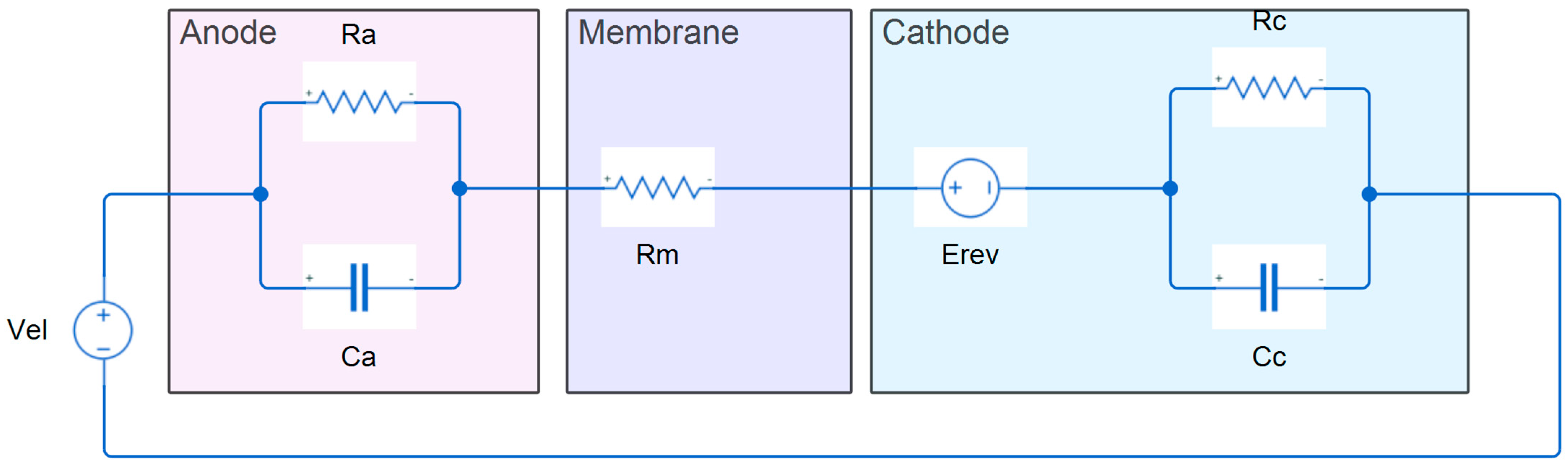
Previous research on PEMELs has shown that electrochemical processes within the internal structure exhibit both dynamic (dynamic operation) and static (steady-state operation) characteristics. This phenomenon of differing operational modes is known as the “double-layer charge” effect. A charge layer, capable of storing charge or energy, exists between the electrodes and the electrolyte. This “double-layer charge” behaves like a capacitor. The accumulation of charges creates an electric voltage corresponding to the activation voltage of the anode and cathode. Consequently, when the PEMEL current changes abruptly, there is a delay before the change manifests due to the activation voltage. Conversely, the ohmic voltage responds immediately to current changes. Based on this behavioral analysis, it is possible to develop an equivalent electric circuit that describes the activation voltage at the cathode and anode.

The model comprises two parallel connections, R_a/C_a and R_c/C_c, representing the anode and cathode, respectively. When a step current is applied to the PEMEL input, the cell voltage, V_el, exhibits primary and secondary transient states. The primary state originates in the anode, where water is supplied. In this state, rapid dynamic changes occur, specifically a rapid increase in the electrolyzer voltage, V_el, caused by an increase in the anode activation voltage, V_aa.

Ra models the Gibbs energy and losses at the anode. The secondary state arising at the cathode (R_c/C_c) is slower, which corresponds to electrochemical reactions. The values of C_c and C_a are approximately the same, but the values of R_a and R_c correspond to the necessary reactions at the anode and cathode. The transition resistances are also included in R_a/R_c. Furthermore, Rm represents the transition resistance of the membrane, and the voltage E_rev models the conversion of energy to hydrogen. Then, based on Figure 1, the PEMEL voltage V_el [15,16] is expressed as follows:

V_el = E_rev + V_aa + V_ac + V_m

(1)

The dynamics of the activation voltage of the anode Vaa and the cathode +Vac are described as [16]:

$${\displaystyle \frac{{dV}_{aa}}{dt}}={\displaystyle \frac{1}{C_a}}·i_{el}-{\displaystyle \frac{V_{aa}}{R_a·C_a}}$$

(2)

$${\displaystyle \frac{{dV}_{ac}}{dt}}={\displaystyle \frac{1}{C_c}}·i_{el}-{\displaystyle \frac{V_{ac}}{R_c·C_c}}$$

(3)

where the parameters C_a, C_c, R_a, and R_c correspond to the elements of the equivalent electrical circuit and i_el is the current in the equivalent electrical circuit.

The time constants that represent the dynamics at both the anode and cathode are given by the following relations [16]:

$${\tau }_{akt,a}=R_a·C_a=C_a\left({\displaystyle \frac{V_{akt,a}}{i_{el}}}\right)$$

(4)

$${\tau }_{akt,c}=R_c·C_c=C_c\left({\displaystyle \frac{V_{akt,c}}{i_{el}}}\right)$$

(5)

The voltages caused by ohmic losses in the membrane [16] are expressed as:

$$V_m=R_m·i_{el}$$

(6)

The energy efficiency is expressed as [16]:

$${\eta }_{el}={\displaystyle \frac{P_{rev}}{P_{el}}}={\displaystyle \frac{E_{rev}·i_{el}}{E_{rev}·i_{el}+(R_c+R_a+R_m)}}$$

(7)

In addition to the conversion of energy into hydrogen, the E_rev voltage also expresses the reverse potential (voltage), i.e., the minimum amount of energy that must be supplied to start the chemical reaction in the electrolyzer cell (this is related to the minimum energy for water dissipation).

The reverse voltage E_rev, depending on temperature (T) and pressure (P), is expressed as [16]:

$$E_{rev(T,P)}=E_{rev\left(STC\right)}+{\displaystyle \frac{R·(273.15+T)}{2·F}}·\ln \left({\displaystyle \frac{P}{P_{STC}}}\right)$$

(8)

where E_rev(STC), P_STC = 1 is the reverse voltage and pressure at Standard Testing Conditions. R is the universal gas constant, and F is the Faraday constant.

At STC, the approximate value of the ideal voltage Vi = 1.233 V. Then the hydrogen production rate V_h, as a function of the equivalent circuit current I_EQ(T,P), is defined as [16]:

$$V_h={\displaystyle \frac{6\times {10}^4·I_{EQ(T,P)}·V_m}{2·F}}$$

(9)

$$V_m={\displaystyle \frac{R·(273.15+T)}{P}}$$

(10)

For a multi-cell PEMEL, with series and parallel connected cells n_s and n_p, the equation of the input voltage V_el is defined as [16]:

$$V_{el\left(T,P\right)}={\displaystyle \frac{n_s}{n_p}}·I_{EQ(T,P)}·R_{i(T,P)}+n_s·E_{rev(T,P)}$$

(11)

R_i(T,P) can be empirically expressed as the total internal resistance of the PEMEL, taking into account the increase in contact resistance due to changes in temperature and pressure [16]:

$$R_{i(T,P)}=R_0+k·\ln \left({\displaystyle \frac{P}{P_{STC}}}\right)+{dR}_t·(T-T_0)$$

(12)

where R_o is the PEMEL resistance at STC, k = 0.0395 is the coefficient obtained from the slope of the V-A characteristic in the linear region, dR_t = 3.182 × 10⁻³ is the coefficient of resistance dependence on temperature, and T₀ is ambient temperature [16].

Identification of the Parameters of the Equivalent Electrical Circuit PEMEL

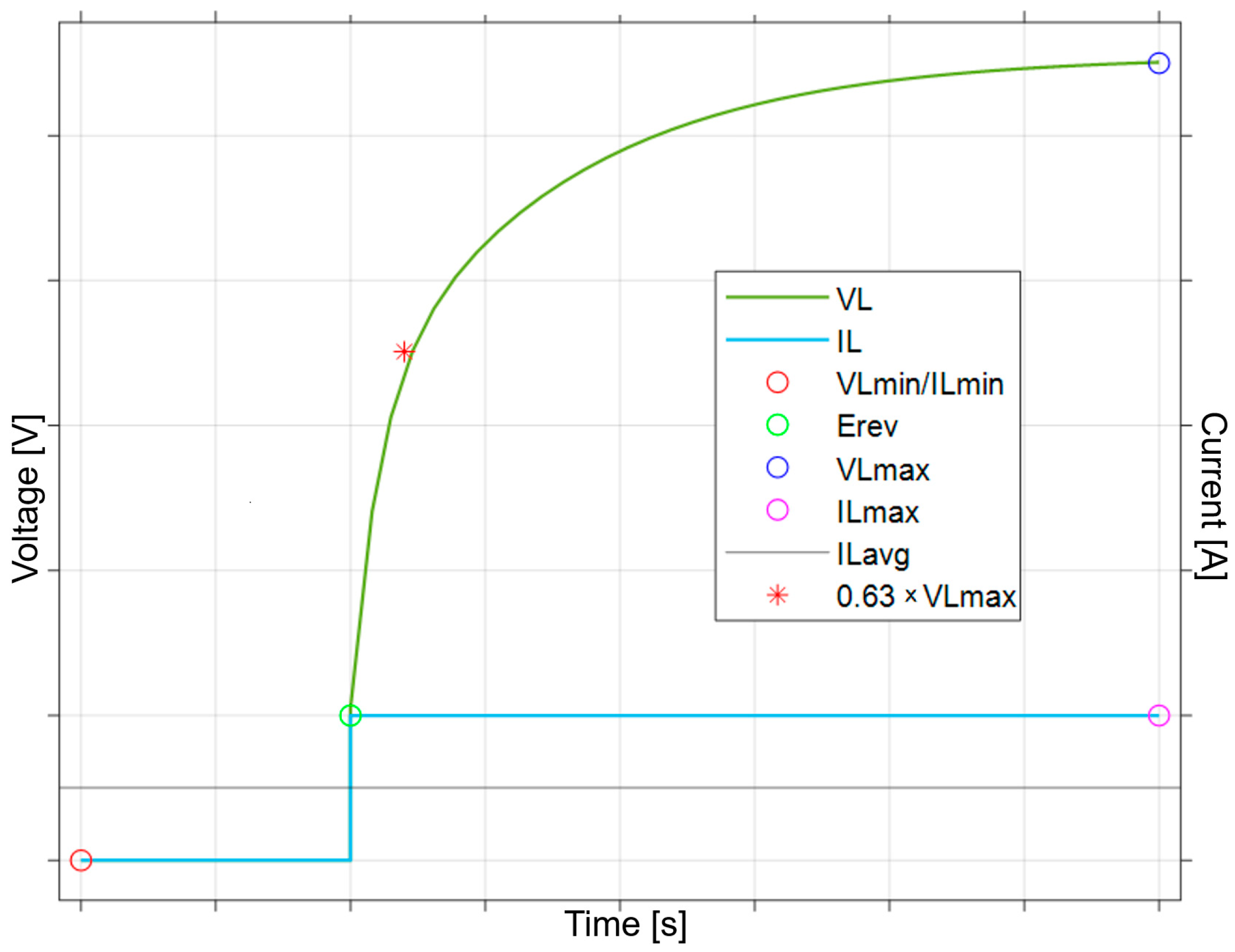
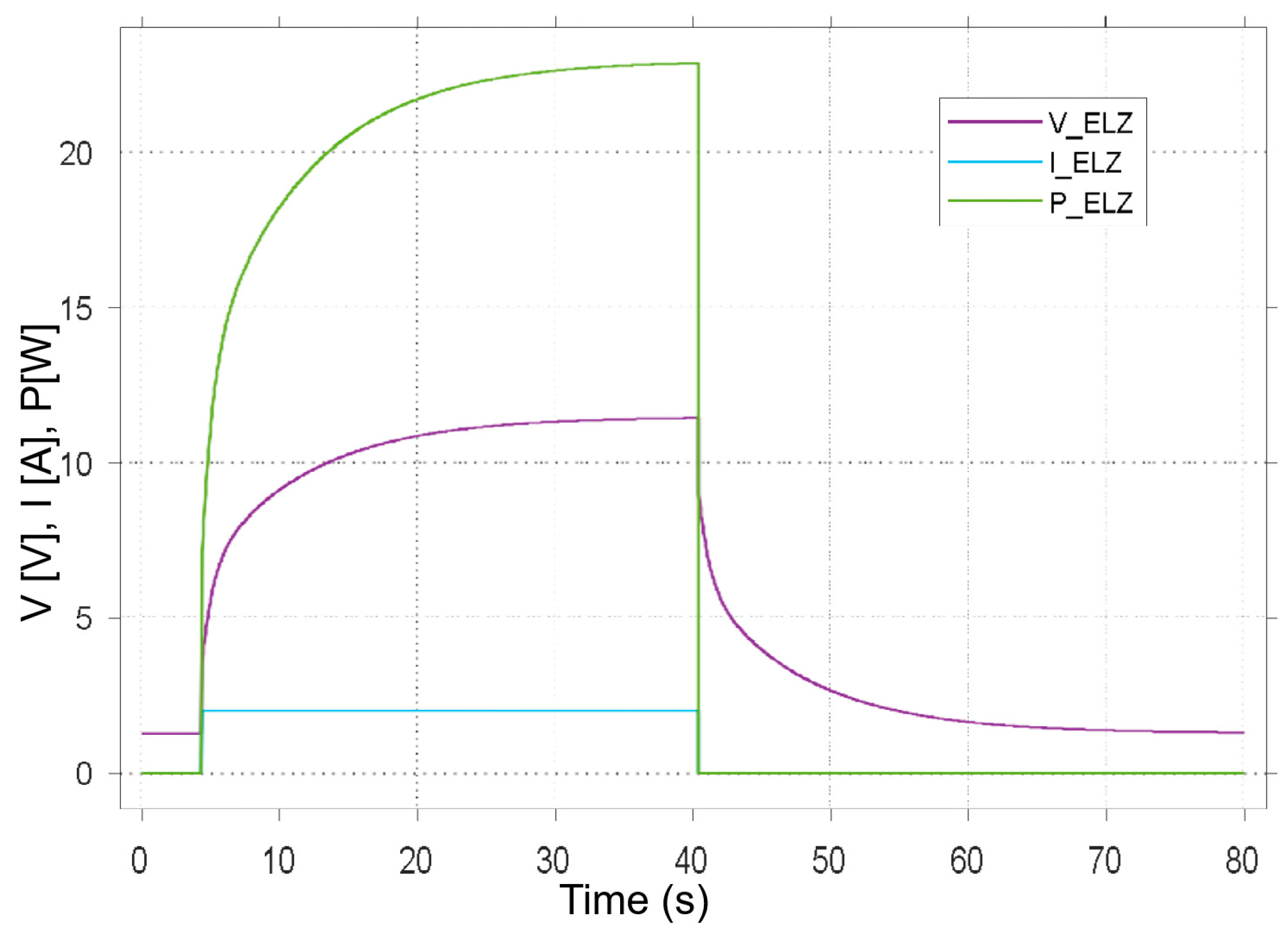
The dynamics, power ramp-up time, and hydrogen production are defined in the equivalent circuit by the parameters R_a, R_c, C_a, C_c, and E_rev. The activation voltage E_rev is a physical parameter of a particular PEMEL. In order for the equivalent circuit to match the real PEMEL, it is necessary to identify the dynamics of the real system. This identification consists of applying a current pulse I_L to the input of the real PEMEL system. As a result of its construction and internal processes, the input voltage V_L gradually increases to its maximum value. Subsequently, the parameters of the equivalent circuit elements are identified from the transient characteristic [16,17].

The total internal resistance of the PEMEL is given by the transient response of the real model [16]:

$$R_{tot}=R_a+R_m+R_c={\displaystyle \frac{V_{L,max}-V_{L,min}}{I_{L,max}-I_{L,min}}}$$

(13)

Then the internal resistance of the membrane [16] is expressed as follows:

$$R_m={\displaystyle \frac{V_{L,min}-V_i}{I_{L,min}}}$$

(14)

where V_i = 1.233V is the minimum Gibbs voltage for water dissipation in PEMELs.

The capacitor value C_a models the fast transients at the anode, while C_c models the slow events at the cathode, which are expressed by the time constants [16]:

$${\tau }_a=R_a·C_a$$

(15)

$${\tau }_c=R_c·C_c$$

(16)

The time constants are subtracted from the transient characteristic (Figure 2) [16]:

$${\tau }_a=0.63·t_{V(L,max)}$$

(17)

$${\tau }_c=t_{V(L,max)}-0.63·t_{V(L,max)}$$

(18)

where t_V(L,max) is the time for which the maximum voltage PEMEL V_L,max is reached, and 0.63 × t_V(L,max) expresses the time for which 63% of the maximum voltage V_L,max is reached after the current pulse. By dividing the total resistance R_tot between the membrane, anode, and cathode, the corresponding values of the capacitances C_a, C_c, determining the dynamics of the PEMEL system, are calculated [16,17].

3. Modeling of Clustered PV Panels

The cells are connected in series to elevate the voltage output. Subsequently, these series strings are connected in parallel to attain the desired current level. The interconnected cells, along with their electrical connections, are then sandwiched between a transparent top layer, typically glass or clear plastic, and a durable bottom layer, such as plastic or metal. An external frame is incorporated to enhance the mechanical integrity of the assembly. This structure is referred to as a PV module or panel, which serves as the foundational component of PV systems. Partial shading can drastically diminish the power output of a PV system built from these panels. Therefore, diverse arrangement and reconfiguration strategies have been introduced to lessen the impact of partial shading. The aim is to identify a connection topology that effectively compensates for variations in light intensity and maximizes system suitability.

Basic ways of configuring PV panels, considering the influence of different solar radiation, include the following:

• Series–Parallel connection (Ser-Par)
• Total-Cross-Tied (TCT)
• Total-Cross-Tied with Current Compensation (TCT-CC)
• Master–Slave connection
• Bridge linked
• Honeycomb

To verify the behavior of the above-mentioned topologies in poor lighting conditions, a simulation scheme consisting of 25 panels was compiled in the Matlab-Simulink simulation environment. Connecting multiple panels is necessary to verify the effect of different radiation on the system. The panels were arranged in a 5 × 5 pattern.

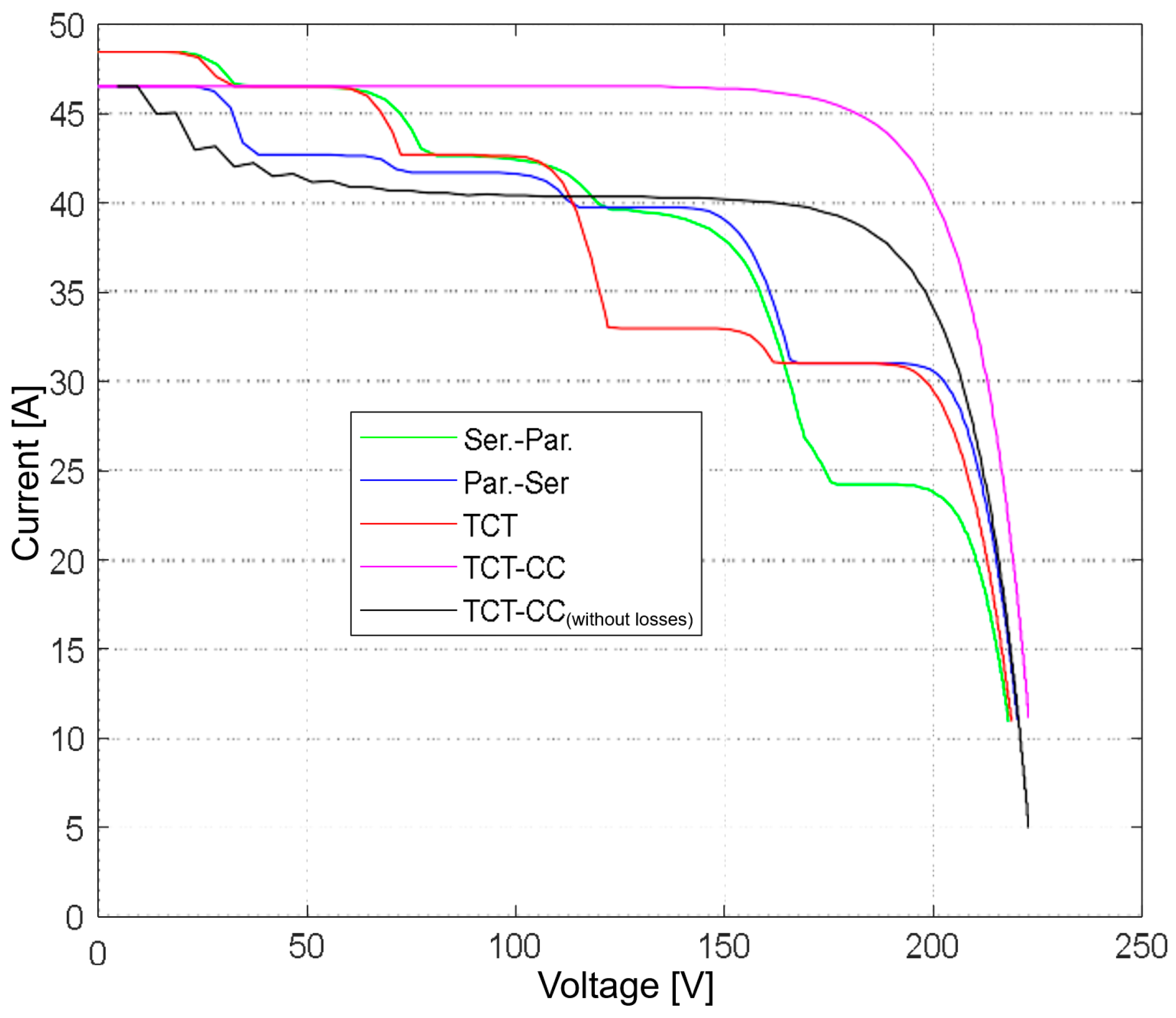
The solar radiation was different on each of the panels in the range of 200–1000 W/m², which, in a real system, can simulate the effect of weather (passing clouds) or shading caused by other objects. Figure 3, below, shows the V-A characteristics of the simulation system of 25 panels. In the first two connection cases, Ser.-Par. and Par.-Ser., we see that the V-A curve has a “cascade” character, which is caused by the different radiation.

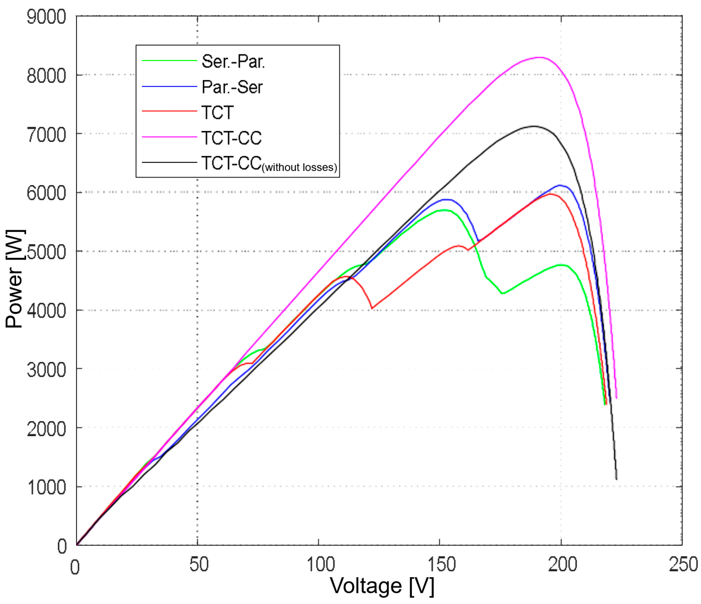
The five “cascades” represent five parallel connections of five panels in series. Due to varying irradiance, these cascades produce differing current values. Even with a TCT (Total-Cross-Tied) topology, current drops occur. However, the TCT-CC (Total-Cross-Tied with Current Compensation) topology eliminates cascade drops by compensating for these current discrepancies. After accounting for the power required by the system, this topology demonstrates superior energy yield. The P-V characteristic shown in Figure 4 validates these results. The area under the P-V curve serves as the primary optimization criterion; a larger area indicates greater energy output and overall system efficiency. Furthermore, current or power discontinuities adversely affect MPPT. MPPT algorithms often converge on local maxima of the P-V curve, necessitating advanced techniques to identify the global maximum.

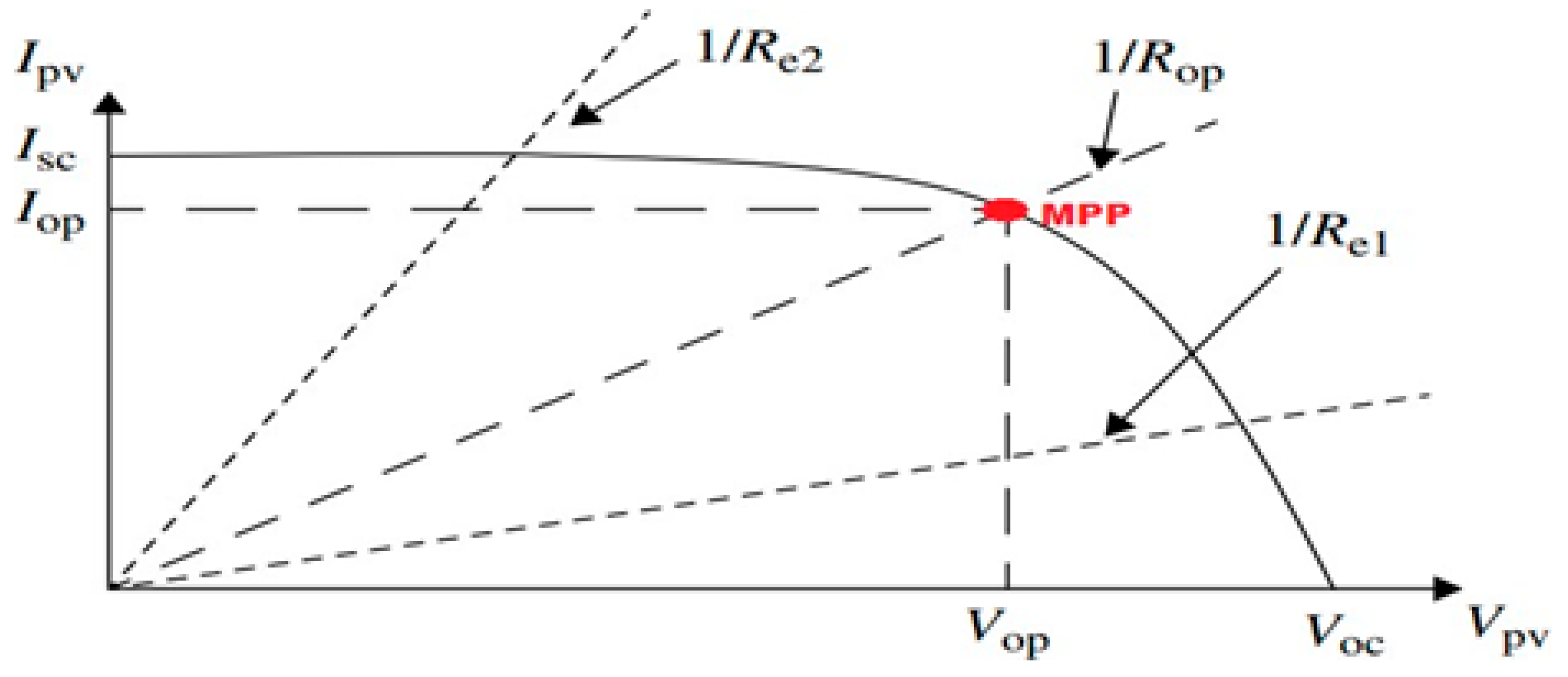
PV systems utilize DC/DC converters for both voltage transformation and MPPT. The output current and voltage of a PV panel are dependent on the duty cycle of the DC/DC converter. If a PV system is directly connected to a load, such as a battery, the operating point is established at the intersection of the PV panel’s voltage–current (V-I) curve and the load’s V-I curve. This operating point may be considerably distant from the maximum power point (MPP) where the PV panel delivers its peak power. Consequently, MPPT optimization methods are implemented to adapt the load characteristics to changing environmental conditions by modulating the converter’s duty cycle, which directly influences the PV panel’s output voltage. Temperature variations primarily affect the output voltage, whereas solar irradiance fluctuations primarily affect the output current. To ensure optimal performance, PV systems must be designed to consistently operate at the MPP across a wide range of temperatures and irradiance levels. Additionally, the load resistance, which is typically not constant, plays a crucial role in determining the PV output power. The maximum power transfer is achieved when the load resistance equals the PV panel’s internal resistance.

To determine the optimal operating point of voltage and current I_op and V_op, a DC/DC converter is inserted between the PV array and the load. A controller is also connected to the DC/DC converter, which, by implementing the MPPT algorithm, ensures the operation of the PV array at its MPP. The controller has the task of calculating the inverter duty cycle, i.e., the ratio of the inverter output voltage to the input voltage. The location of the MPP (Figure 5) is not known a priori, but it can be traced using MPPT algorithms [18,19,20,21].

3.1. Direct Methods

Direct methods use real measured quantities on the PV panel to estimate the MPPT, i.e., voltage, current, and temperature. Direct methods have the advantage that they are independent of the characteristics of the PV panel, so it is not necessary to know the exact parameters of the PV panel or the current state of degradation. Direct techniques include differentiation, feedback voltage, disturbance and observation (P&O), incremental conductance (IC), fuzzy logic, and artificial neural networks.

3.2. Indirect Methods

Indirect methods are based on the use of a parameter database that includes data on the V-A characteristics of the PV panel at different radiation and temperature, or are based on the use of mathematical functions obtained from empirical data. In most cases, mathematical relationships obtained from empirical data are used.

4. Scaled-Down Model

The following sections summarize the information on the design and assembly of a scaled-down model of the system, which will be able to direct energy from 4 PV panels to a Li-ion battery storage, and then directly to a separate Horizon Hydrofil Pro electrolyzer system. The scaled-down model serves to collect data on the principle of operation and control method. The measured data is then used for the simulation design of a system with PV panels with a power of 100 kWp, a battery storage with a capacity of 660 kWh, and an electrolyzer, enabling hydrogen production with energy consumption ranging from 33 to 100 kW.

The scaled-down system consists of an Arduino Mega 2560 control unit, XL6009 power converters, ACS712 current sensors, voltage sensors, temperature sensors, switching relay elements, protective diodes, and fuses. The battery storage contains 8 Panasonic 18650GA cells with a total nominal capacity of 27.6 Ah (100 Wh) and an output voltage range of 5 to 8.4 V. The PV source consists of 4 monocrystalline Cellevia PV panels with a nominal power of 20 W and a total power of 80 W. Furthermore, the system includes preparation for connecting a fuel cell via Arduino Uno.

The aim of the design in the next steps is also the possibility of autonomous operation; therefore, the system is equipped with a NodeMCU communication unit, which allows the system to connect to the Internet via WiFi and share information about the system status.

4.1. Electrolyzer

The simulation model of the electrolyzer is based on a real device for hydrogen production using PEM electrolysis, designated as the Horizon Hydrofil Pro FCH-020. The input to the system is deionized water and electricity. PEMELs can be operated on energy produced from renewable energy sources. The produced hydrogen is stored in a metal hydride tank AB5 with a capacity of 10 L at a working pressure of 3 MPa and a temperature of 0 to 55 °C.

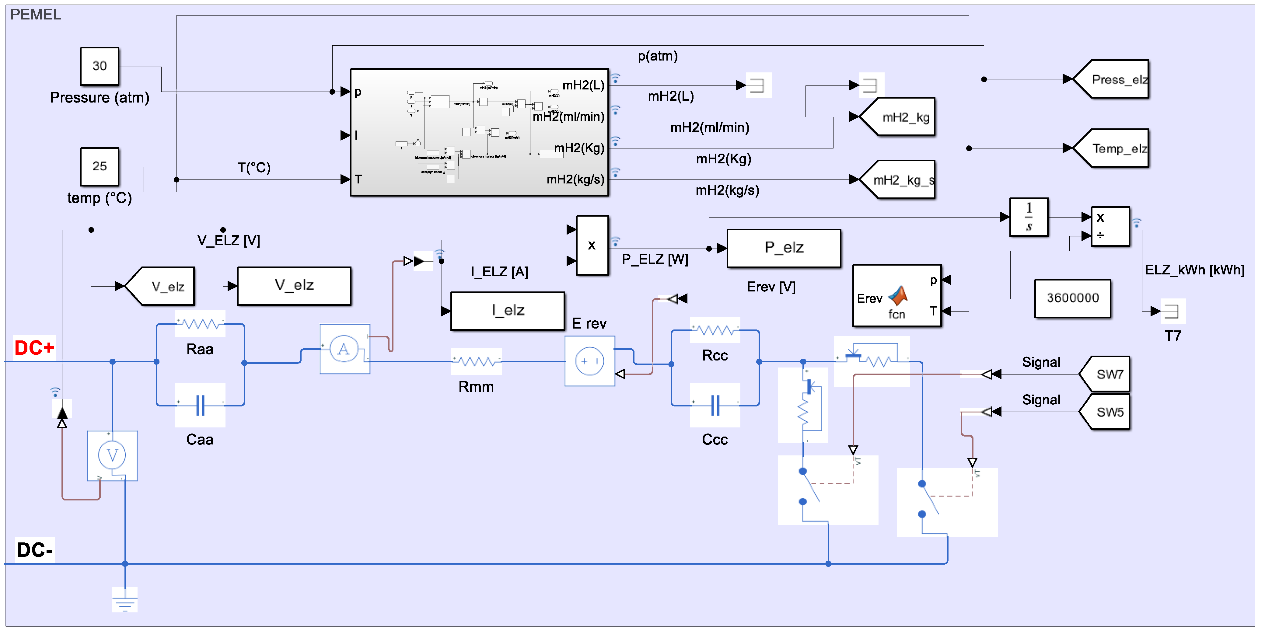
PEMELs represent a system where chemical reactions also take place, which do not need to be modeled for energy analysis. The complex PEMEL FCH-020, which also includes a system for flushing, preheating, humidifying, and dosing water into the membrane, is replaced by a model based on an equivalent electrical circuit (Figure 6).

4.2. PV Panel

The voltage and current at Pmax determine the operating point at which the PV panel produces the highest power (Figure 7). This point does not change only with changes in radiation but also depending on temperature. The increase in the operating temperature of the PV panel is caused by the course of the photoelectric effect on the diode and the increase in external temperature. The dependence of the increase in the internal temperature of the PV panel on the ambient temperature and radiation is linear and depends on the thermal coefficients V_oc, I_sc, and P_PV. The better the material from which the PV cell is made, the smaller the coefficient, and the PV produces higher and more stable amounts of energy. The NOCTs (normal operation testing conditions) express the operating temperature at the STC (Standard Testing Condition).

4.3. Controlling a PV System Using a Mathematical Model: Look-Up Table

The proposed PV system operates in a defined range of input radiation (0 to 1000 W/m²), temperature (−10 to 80 °C), and output voltage (0 to 23 V), and based on this, a mathematical model was created, which is used to calculate the voltage and current values at which either the highest power or the power required for the load will be produced.

The input to the controller is the average value of the radiation and temperature at which the PV system operates. Using the n-dimensional lookup table POWER, a 2-dimensional P-V characteristic is selected for the current radiation and temperature. The ideal PV characteristic has only one global maximum, i.e., one max. power value. This value is indexed with the current value from the CURRENT table, which contains V-A characteristics calculated based on radiation, temperature, and voltage range. The optimal value of the output voltage of the PV system for the given conditions is calculated as a ratio of the maximum power and the corresponding current. Subsequently, the duty cycle for the buck–boost converter is calculated. The duty cycle is controlled by the pulse width modulation (PWM) modulator, whose output is the control signal of the switching elements of the main DC/DC converter.

The Look-Up tables contain, in this case, a 4-dimensional data matrix [V, P/A, G, T] and, in addition to selecting a specific value at the position [x, y, z, k], they allow linear, Lagrange, cubic, and Akima interpolation. This control method is easy to design, and in the case of interpolation, the table does not have to be large in size to maintain the required control quality. The controller defines the exact value of the input voltage of the inverter, which does not oscillate around the desired value, as in the case of digital controllers. The quality of the control is how accurately the mathematical model of the PV panels is built and how accurately the input values of the radiation and temperature are measured.

4.4. Optimizing Energy Production of PV Panels Using MPPT Algorithms

In the simulation model, optimizers are used to connect the PV panels. The optimizer consists of a DC/DC converter that is adapted to the power of the PV panel. The optimizer contains switching elements that disconnect the PV panel when it is shaded or damaged, thereby increasing the efficiency of the entire system, since in a series connection, the current in the chain has the same value as the PV panel with the lowest current production. Unlike the main DC/DC converter, which optimizes the power of the entire PV system, the duty cycle of the DC/DC converter in the optimizer is controlled by optimization MPPT algorithms that increase the efficiency of each panel individually. The optimizer, therefore, contains control circuits and optimization algorithms that evaluate the duty cycle of the DC/DC converter implemented in the optimizer based on continuous measurement. In this work, two MPPT algorithms were used, which are based on the numerical principle. The Perturb and Observe (P&O) and incremental conductance (IC) algorithms are actually used in control controllers, as they are designed to be computationally inexpensive.

P&O is implemented in the Matlab-Simulink environment as a Matlab function script. The input is the voltage V(k) and the current I(k), from which the power P(k) is calculated and then compared with the previous value P(k − 1). Then, the difference between the voltage ΔV and the power ΔP is calculated. Then, it is decided whether the point with the maximum power is to the left or to the right of the current point of the P-V characteristic. The duty cycle value is increased by ΔD, and the value of the current I(k + 1) and the voltage V(k + 1) are measured again. The P&O flow chart is supplemented with hysteresis in the simulation environment to prevent oscillations around the MPP.

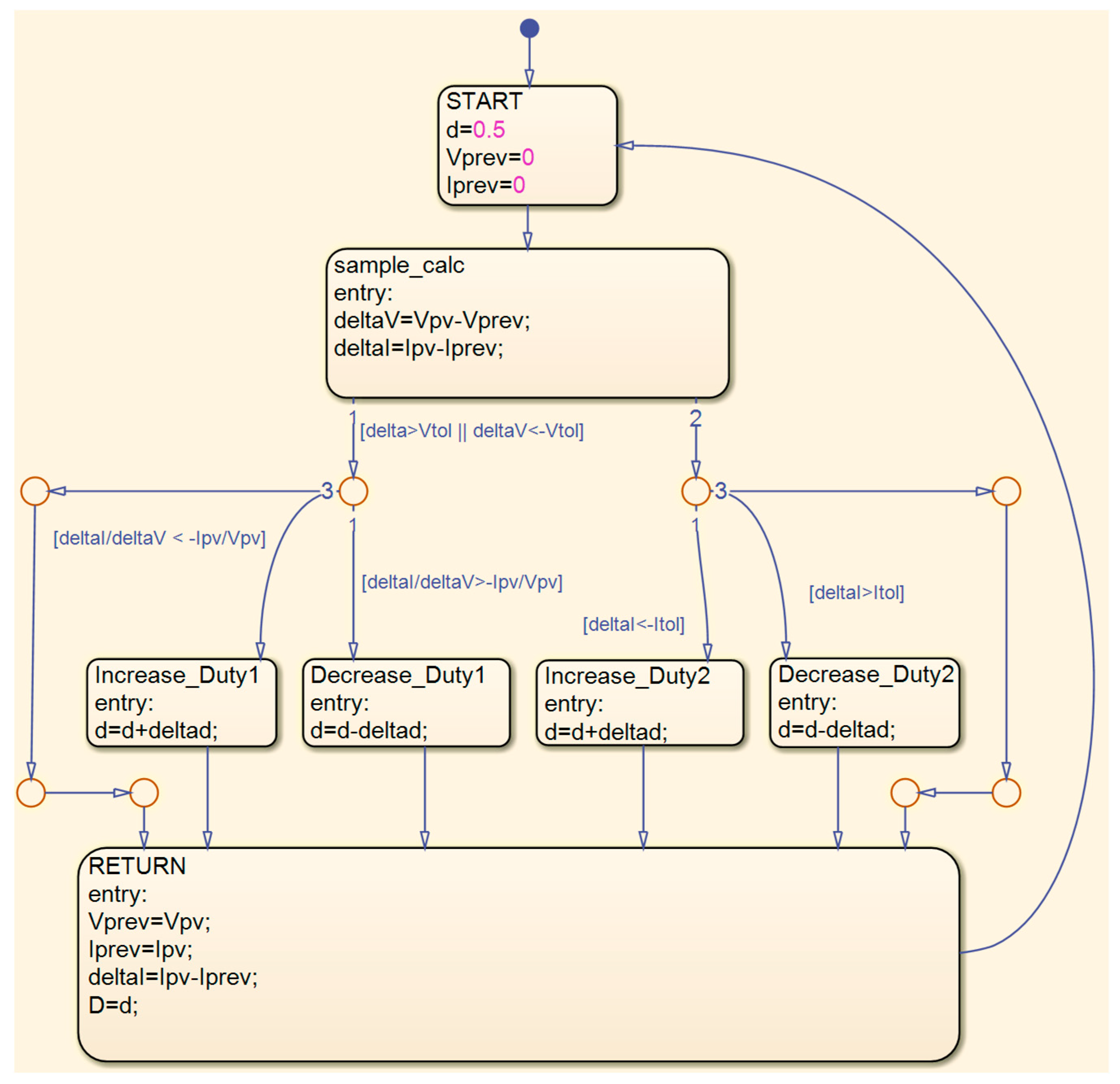
The IC is implemented in the Matlab-Simulink environment as a flow chart in the graphical language Stateflow (Figure 8). Stateflow allows for control design, task planning, and combinatorial and sequential logic that can be simulated as an object. The advantage is the graphic and tabular animation of state changes during the control process, which facilitates the implementation of the control algorithm.

In the first step, the difference between the current ΔI and the voltage ΔV is calculated. Hysteresis, i.e., the tolerance value of the voltage V_tol, is included here. If the voltage increase/decrease is less than this value, the duty cycle D does not change. Otherwise, the duty cycle D changes according to conditions, based on the ratios of the differences to the measured values.

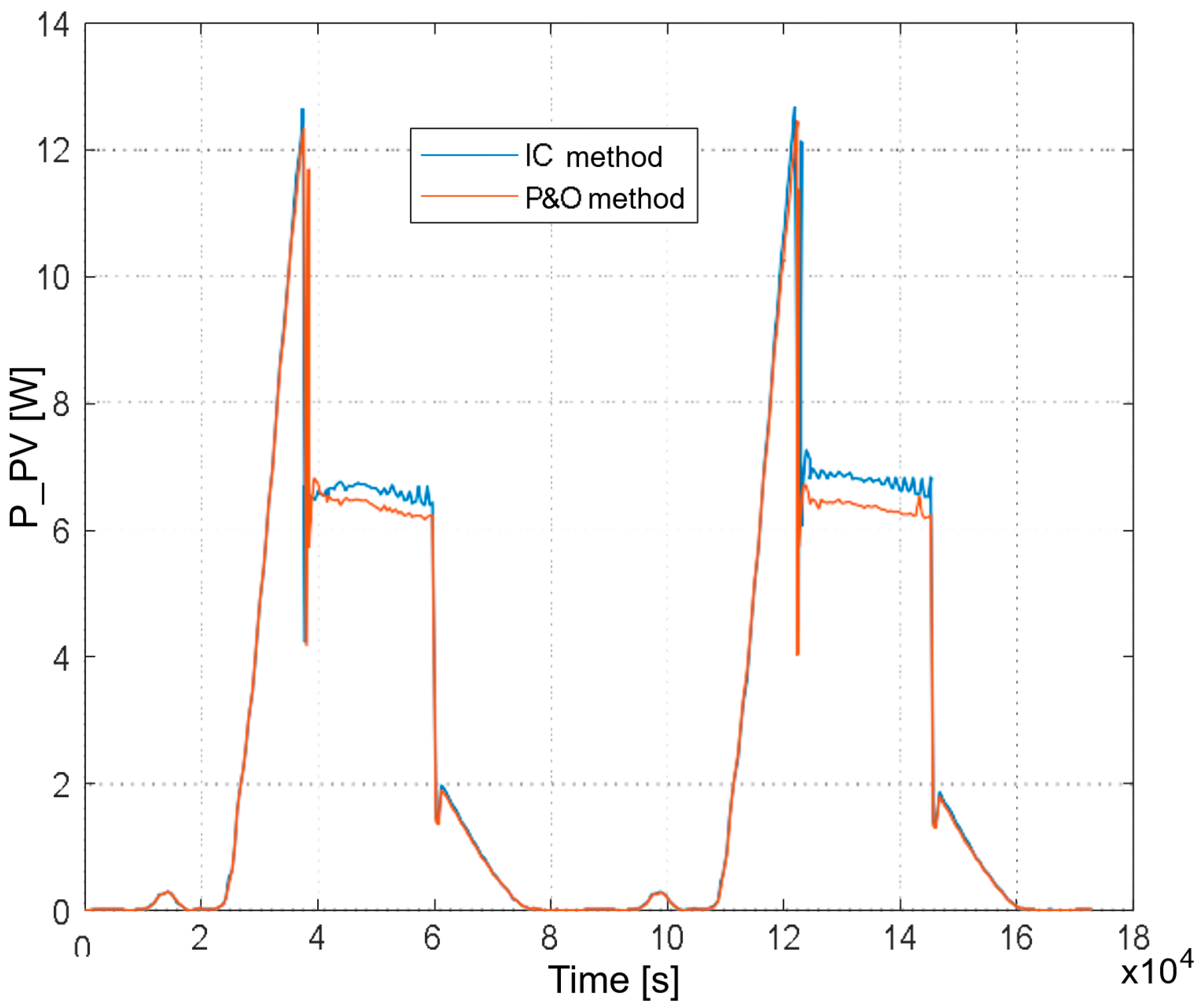
Figure 9 shows the effect of using an optimizer with the IC and P&O control algorithms on the performance of one CL-SM20M panel in a simulation model of an 80 W system. The curve simulates the system’s operating cycle for 2 days. After the battery is charged, the load (battery–electrolyzer) changes. This is where the IC method responds better to the change, unlike the P&O method, where convergence occurs later. Also, at higher powers, the P&O method oscillates around the operating point P_PVmax = 15 W, and the IC method converges to the operating point and P_max = 17 W.

4.5. Controlling the Power of PV Panels When Powering the Electrolyzer

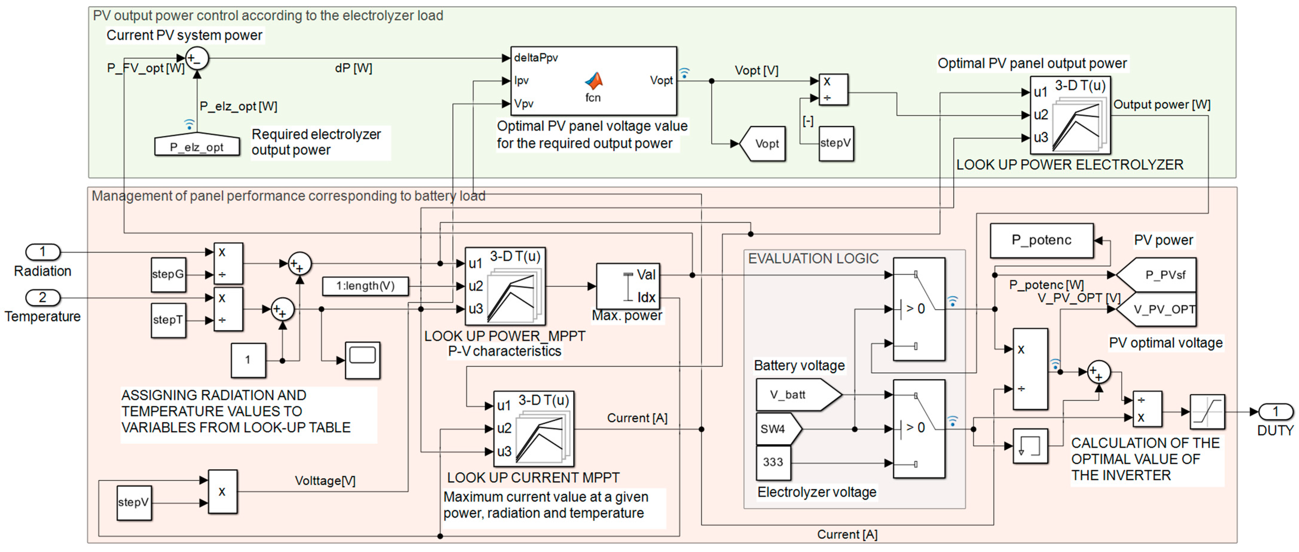
When the electrolyzer is powered only from the battery, the inverter duty cycle is calculated based on the voltage of the electrolyzer and the battery, and the total power drawn from the battery is limited by the current consumption of the electrolyzer. When powered purely from PV panels, their output voltage is unstable and it is necessary to limit the produced power, since the PV produces a maximum of 80 W and the electrolyzer consumption is 23 W. The limitation is implemented by shifting the operating point of the PV system’s P-V characteristics to the value of the required power. The control circuit uses a Look-Up Table (Figure 10). The required electrolyzer power is subtracted from the current PV system power, and the difference, together with the current voltage V_PV and current I_PV, enters the function where the optimal voltage value V_opt of the PV system is calculated from the power difference ΔP_PV. This value is assigned the optimal PV power value based on the current radiation and temperature. The power is further converted to the voltage and duty cycle of the inverter D. This control ensures that even with a potential PV system power of 80 W, the maximum output power will be 23 W. This control is only allowed if the produced PV power does not fall below the required electrolyzer power limit.

4.6. Decision Logic for Energy Flow Management

The PDU (Power Distribution Unit) provides the energy flow from the PV system to the battery and the electrolyzer. The PDU contains three relays in the case of the 80 W simulation model.

The relays are connected to enable all possible combinations of the system’s operating cycle:

• Battery charging from the PV system.
• Battery charging and electrolyzer power supply from the PV system, simultaneously.
• Electrolyzer power supply from the PV system.
• Electrolyzer power supply from the PV system and the battery, simultaneously.
• Electrolyzer power supply from the battery.

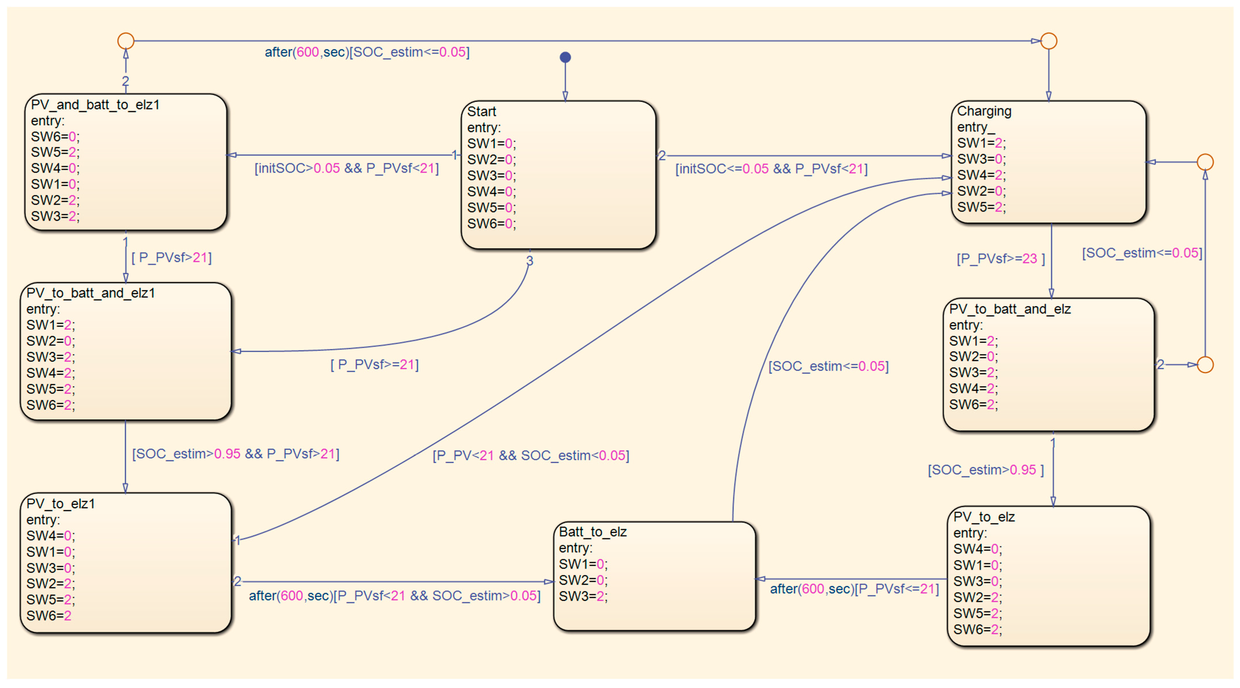
The control signal for controlling the relay will be implemented in the simulation model as in the real system, namely by the voltage threshold value V_thld 0–5 V. The signal is generated in the control unit. The evaluation logic in the simulation model is implemented by the graphical language Stateflow. In the real model, the control system in Simulink will be transformed using Matlab Simulink Coder and Embedded Coder into C, which allows for high interoperability between the control development and implementation in microcomputer control systems. The input variables to Stateflow are the initial battery State Of Charge (initSOC), the optimal PV system power value (P_PVsf), and the calculated battery State Of Charge (SOC_estim).

The control process initiates at the Start block (Figure 11), setting all control voltage values for switching elements SW1 through SW7 to zero. The system is designed to operate regardless of the battery’s initial state, whether fully discharged or partially charged. In the event of a fully discharged battery and insufficient PV power to activate the electrolyzer, a battery charging cycle is initiated. During this phase, energy from both the battery and the PV array is directed to the electrolyzer. When PV power exceeds the electrolyzer’s power consumption, the surplus energy is used to charge the battery while simultaneously supplying power to the electrolyzer. Upon reaching a full battery charge, and with adequate PV power available, the electrolyzer is powered directly. Conversely, if the PV’s power drops below the electrolyzer’s minimum operating level, the fully charged battery supplies the required power. This control logic is also implemented when the battery is partially discharged. The complexity of the system, with its numerous variables, makes it difficult to account for every possible operational scenario. Nevertheless, the overarching control priority is to ensure continuous operation of the electrolyzer, thereby guaranteeing a stable hydrogen production rate.

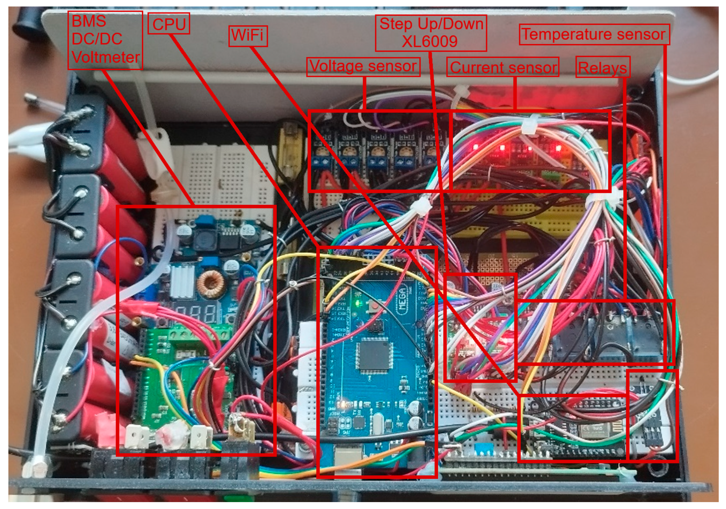
4.7. Testing the Built Model

Figure 12 shows the system set up during testing. PC is used for control and graphical evaluation, instead of autonomous operation. Four PV panels are connected to the system.

The waveform in Figure 13 shows the performance of the battery, electrolyzer, and PV system. The PV system’s performance is not optimal due to the absence of an MPPT algorithm. Despite this, the system is able to deliver 17 W of power to the battery and electrolyzer. It is important to note that this scaled-down model served primarily to verify the behavior of the PV panels. An MPPT algorithm would optimize the PV system’s performance by tracking the maximum power point, resulting in higher efficiency.

Figure 14 shows the performance of the PV system when powering the electrolyzer without a battery. A perfectly stable PV system performance was achieved, with zero shading of the PV panels and a clear sky.

4.8. Implementation of the MPPT Optimization Algorithm into the Scaled-Down Model

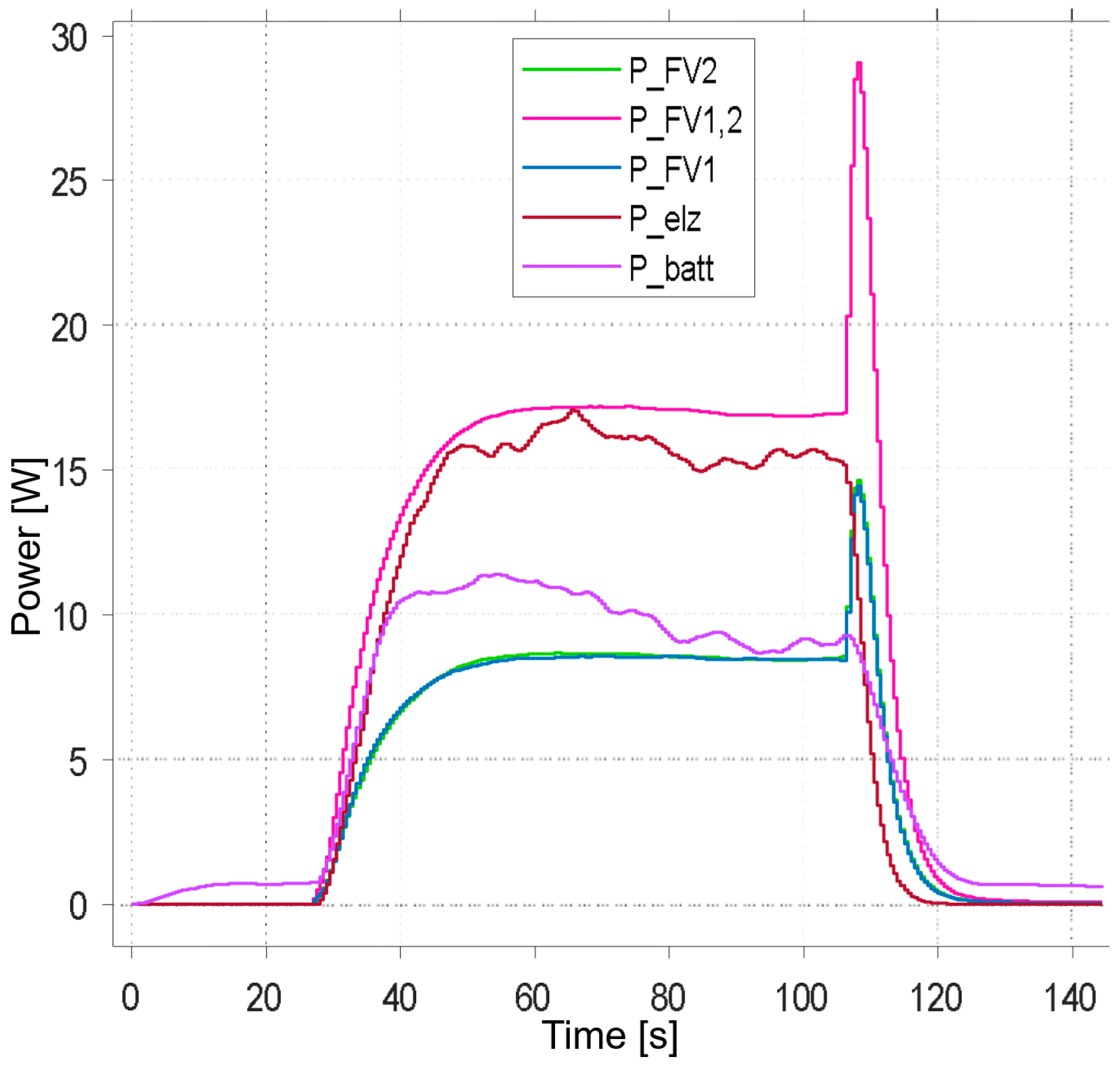
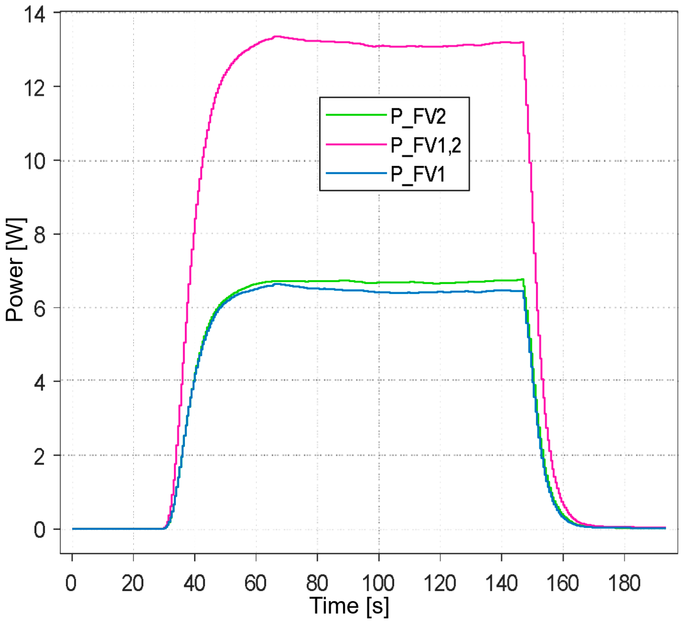
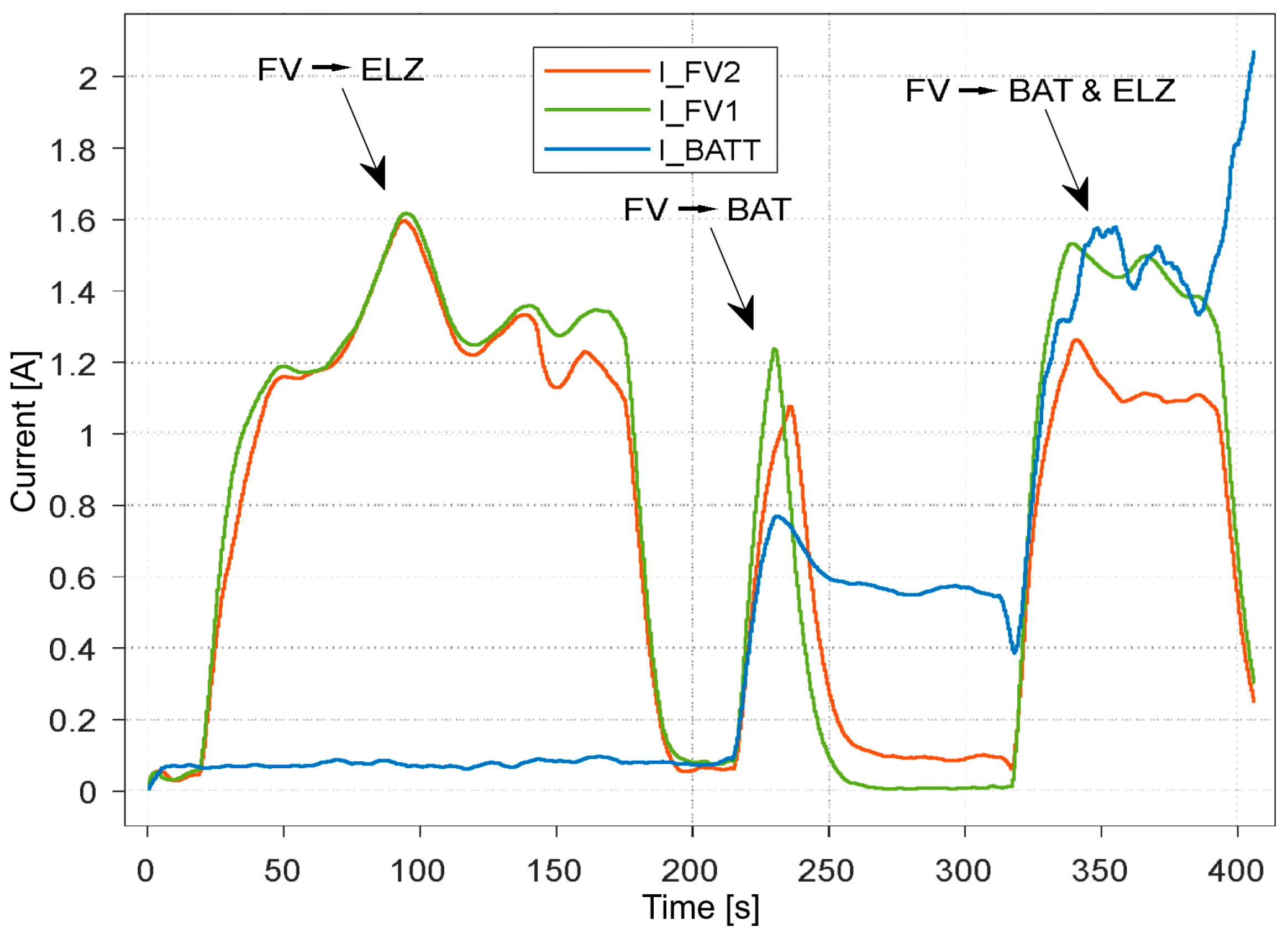
For testing purposes, the PEMEL was replaced by a programmable power load, simulating the transfer of the produced PV power. In Figure 15, the power load (PEMEL) from the PV system is supplied in the first part. Four panels were divided into two parallel connections, i.e., one panel produced an average of 0.6 out of 1.12 A (at full radiation of 1000 W/m²). Since the relationship between the current and radiation is linear, according to the V-A characteristics of the panel, the value of the produced current corresponds to radiation of 530 W/m², which almost coincides with the NREL radiation data for the month of September.

Furthermore, in the case of battery powering from PVs, the operating point of the PV system will shift to the right. Subsequently, when the battery and the electrolyzer are connected, the voltage ratios at the inverter output will change, and the operating point will shift to another area.

The result is that the produced currents are sufficient, but the PV panel voltage needs to be maintained at an optimal level using the MPPT algorithm and the inverter.

5. Design of a Hydrogen Production System for a Specific Application with a Power of 100 kWp

This section details the design procedure for an energy system featuring a 100 kWp maximum output PV system, a 660 kWh battery storage, and an electrolyzer enabling hydrogen production, with an energy consumption ranging from 33 to 100 kW. The design utilizes real-world components and considers their physical properties.

The PV panel selected is the TALESUN TP7F78M, a monocrystalline, half-cell module designed to minimize the impact of varying irradiance across the panel surface. The PV array consists of 8 parallel strings, each comprising 21 panels connected in a series. This configuration yields a maximum voltage of 950 V and a current of 13 A per string. The total array generates 105 A, 950 V, and 100 kWp of power. In addition to the internal diodes in the PV panels, bypass diodes are implemented to mitigate string failures due to shading on individual panels, preventing the “hotspot” effect (where a shaded panel acts as a load). The string energy is then directed to optimizers, where the power output is maximized using the MPPT. Blocking diodes ensure unidirectional current flow from the individual strings to the main inverter.

The simulation design incorporates the real NEL C SERIES C20 PEM electrolyzer system (Figure 16). Beyond the PEM cell, the actual system includes a heat exchanger, a gas detector, a separator, and hydrogen and oxygen phase dryers. At an electrolyzer operating power of P_EL = 120 kW, 43.3 kg of hydrogen (H₂) is produced per 24 h. Given hydrogen’s energy density of 33.3 kWh/kg, this equates to 1441.89 kWh of stored energy in the form of hydrogen. The production consumes 2880 kWh of electrical energy, confirming an electrical-to-hydrogen conversion efficiency of 50%. The remaining thermal power (P_heat) is dissipated through cooling in the heat exchanger.

The requirement for the storage design is to ensure the operation of the PEMEL at a third of the power, i.e., 33.3 kW for 10 h, so that the battery capacity does not fall below 50%, or the operation of the PEMEL for 20 h when the storage is completely discharged, which corresponds to a capacity of 660 kWh. The power of the PEMEL is limited to a third in the simulation scheme when powered by batteries, which extends their service life, as the current requirements are reduced. Thus, in addition to the capacity, the battery storage must be at a similar voltage and current level as the energy source and consumer, i.e., the PV system and the PEMEL. Based on previous knowledge, we will choose a LiFePO₄ battery for storage instead of Li-ion cells, which would have to be in large numbers to achieve the necessary capacity, which increases the failure rate and space and weight requirements, since the Li-on connection system makes up a part of the weight of the entire battery.

LiFePO₄ has a large capacity, sufficient charging and discharging currents, and a voltage range similar to other Li-ion cells. Since it is used in stationary applications, weight is not a limiting parameter, and the shape allows for compact grouping into units.

5.1. Total Annual Energy Input of the PV System

The amount of energy produced by the PV system in the compiled simulation design was compared with available software that is used for the design of PV systems for commercial purposes. Specifically, the OpenSolar software (version OS 2.8.0) was used. In this software, a model was created consisting of 168 pcs of the same TALESUN TP7F78M panels. The total energy produced by the design in Matlab-Simulink is 122.69 MWh/year, and is 115.82 MWh/year using OpenSolar software. The difference between the different design methods is 5.6%. The overall difference, but also in the distribution of production by months, is caused by the fact that approximate data are used in the calculation in Matlab-Simulink, unlike OpenSolar, where databases with measured radiation values for a given geographical location are used. However, the difference is negligible, which confirms the correctness of the design.

5.2. Principle of Operation During Periods of Maximum Radiation

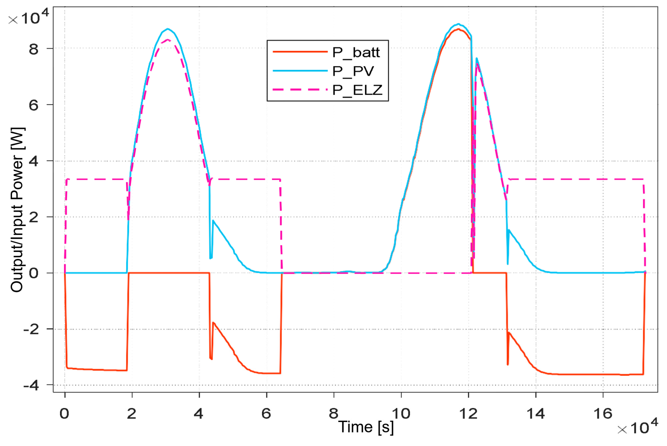
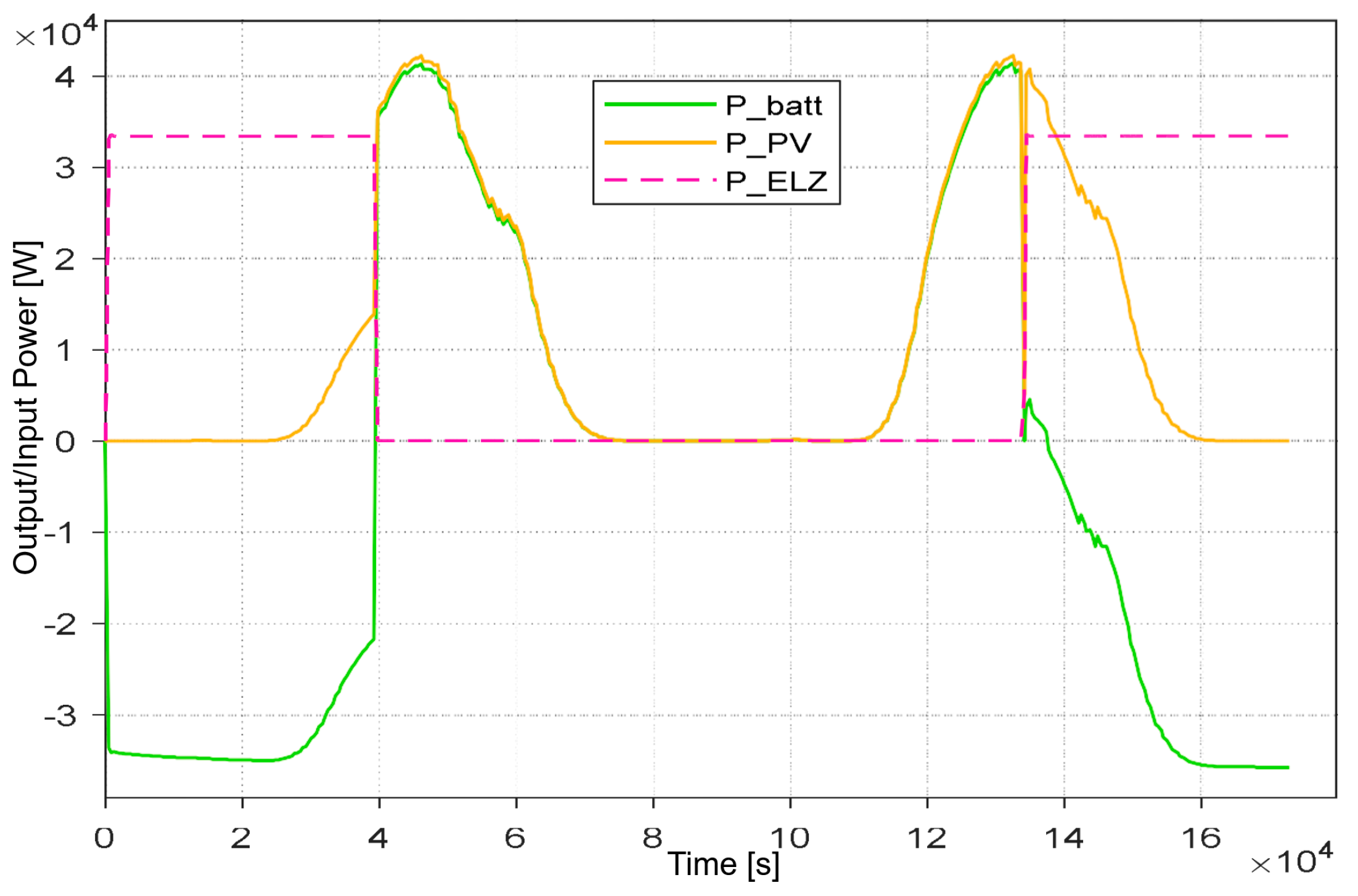
The current of the PEMEL’s power, the PV system’s power, and battery storage for 48 h are shown in Figure 17. Although the potential PV power at 1000 W/m² radiation was 100 kWp, taking into account the ambient temperature and the dependence of the PV panel temperature on the generated energy, the real maximum power was 87 kW at the same radiation on all panels.

At the initial SOC = 100%, the battery first powered the PEMEL for 5.2 h, then, after reaching a PV power > 33 kW, it was disconnected, and the PEMEL power increased, depending on the PV system’s production. At time 6.5 × 10⁴ s, the SOC was <50%, which stopped the hydrogen production. Subsequently, recharging took place. At 12.1 × 10⁴ s, the PV system load changed from the battery to the PEMEL, which caused energy losses; therefore, these changes are not suitable for performing at maximum PV system power. The simulation design takes into account the efficiency of DC/DC converters in the range of 95–98%. The battery power during the PEMEL power supply process increased slightly (from 34.5 to 36.7 kW), even though the PEMEL power input was the same. This is due to the compressor power consumption, which depends on the pressure to which the produced hydrogen is compressed.

5.3. Principle of Operation in the Period of Average Radiation

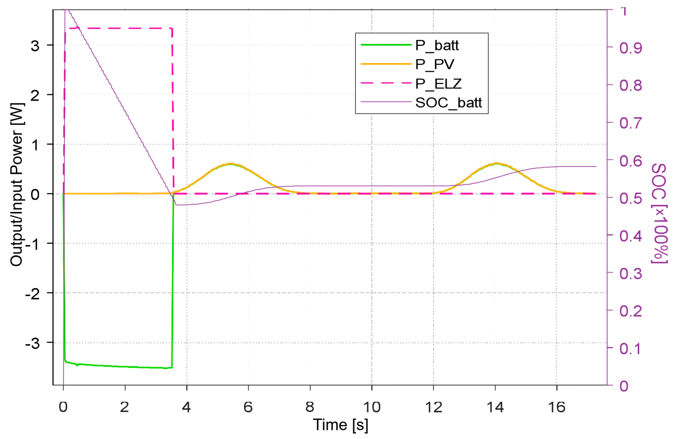
Although the average radiation reaches 500 W/m², the PV system’s performance is not reduced by half compared to the previous test. The maximum PV system’s performance at average radiation is 42 kW. The nonlinear relationship between the output power and radiation is caused by the reduced ambient temperature, which reduces the output voltage (Temperature coefficient V_oc = −(0.26 ± 0.05)%/°C).

The battery in the PV system supplies energy to the PEMEL until the SOC < 50%, i.e., for a period of 4 × 10⁴ s (~11 h), then the battery is recharged to the reference level and, thus, the system can produce hydrogen hybridly. The reduction in the PV system’s performance is supplemented by the battery, which is one of the design goals. The PEMEL operation is optimized to ensure the specified battery charge.

As can be seen in Figure 18, in the first part, the full potential of the PV system is not utilized, as this is due to a partial divergence in the control algorithms and, thus, the PV system does not operate at the maximum power point.

5.4. Principle of Operation During Periods of Minimum Radiation

In winter, radiation is achieved at a level of 140 W/m², i.e., 14% of the maximum radiation in the summer. The maximum power at a minimum radiation of 6 kW, however, is only 6.9% of the power achieved at the maximum radiation, i.e., 87 kW. This is caused by both the negative temperature during the entire test and the lower efficiency of the PV system at a low input radiation.

The system, again, initially produced hydrogen for 3.6 × 10⁴ s (~10 h) and then the battery was recharged for 38 h. Figure 19 shows the performance curve together with the current SOC of the battery. The energy input in the PV system is low for both hydrogen production and battery charging. After the initial discharge to the level of SOC = 47%, only 10% of the obtained energy was charged, i.e., SOC = 57%, i.e., 66 kWh.

In winter, the storage capacity is, therefore, unused, and the hydrogen production is limited to only one source—the battery. In island operation, it is necessary to maintain the battery temperature in an acceptable operating temperature range between 10 and 60 °C and to take into account self-discharge. After taking these parameters into account, the difference between the obtained and stored energy could be negative.

6. Economic and Ecological Comparison of the Simulation

For reference, in the simulation results, we compared the economic and ecological impact of transportation. Hydrogen production, using our simulated system, which utilizes PV panels with a capacity of 100 kWp, was compared to conventional energy sources currently used in urban public transport across Europe.

For the calculations, we used a real model of the Solbus SM12H2F hydrogen-powered bus, which is in operation in various European cities. This allows us to directly compare the simulation results with real-world operation. The bus is equipped with a 37.8 kWh battery; however, this battery does not influence the calculation, as it serves only as a temporary storage to balance power peaks.

The technical specifications of the selected vehicle are presented in

Table 1. Technical specifications of Solbus SM12H2F.

Parameters	Solbus SM12H2F
Range	450 km
Hydrogen refueling time	15 min
Hydrogen tank pressure	350 bar
Hydrogen capacity	30 kg
Fuel cell	HyMove Fuel Cell System 60 kW
Nominal power	226 kW
Maximum power	364 kW
Drag coefficient	0.4
Dimensions	12,000 × 2500 × 3100 mm
Weight	12,550 kg

.

The input to the simulation consists of defined relations for calculating the resistances acting against the movement of the vehicle. The simulation then calculates the bus consumption per 100 km for a specified driving cycle. The consumption is reduced by the value of the recuperated energy, i.e., during braking, the fuel cell is idle, and the recuperated energy is stored in the battery. The consumption of the Solbus bus during the UDDS cycle is 120.8 kWh.

Various driving cycles are used to calculate standardized consumption. The differences are mostly in the average speed, distance, acceleration, and stopping time. The cycles are further divided based on the type of tested vehicle (van, passenger car, and truck) and driving profile (city, highway…).

Table 2. Overview of Solbus SM12H2F consumption during driving cycles.

Driving Cycle	Electric Energy Consumption kWh/100 km	Hydrogen Consumption kg/100 km
NEDC	137.20	8.24
ECE R15	130.83	7.85
EUDC	140.92	8.46
ArtUrban	166.83	10.02
ArtRoad	128.61	7.72
ArtMw130	139.55	8.38
ArtMw150	143.38	8.61
WLTP	115.30	6.92
UDDS (HHDDT)	120.80	7.25
FTP	121.00	7.26
HWFET	91.95	5.52

provides an overview of the most commonly used driving cycles and the simulated consumption of the vehicle with the above-defined parameters. The consumption of el. energy includes losses caused by components of the electric drive, such as converters, engine control units, and motors. The hydrogen consumption is obtained by simulation calculation from the efficiency of the HyMove Fuel cell system at 60 kW, and the standard energy density of hydrogen as 33.3 kW/kg.

Balance of Produced, Consumed, and Stored Energy During System Testing

In

Table 3. Summary of the simulation results for the 100 kWp model.

System Setting	PV	PEMEL	Batt IN	Batt OUT	Batt DIFER	mH2	H2 Energy	Consump. Coverage
Max. rad. SOC = 95%	782	1039	395	−714.7	−319	17	566.1	30.9
Avg. rad. SOC = 95%	504	691	377	−610	−233	11.2	372.9	20.3
Min. rad. SOC = 95%	70.8	335.6	69.3	−350	−281.4	5.1	169.8	9.2
Max. rad. SOC = 5%	1242	832.3	712.7	−356	356.7	14	466.2	25.4
Avg. rad. SOC = 5%	575	0	563.5	0	563.5	0	0	0
Min. rad. SOC = 5%	70.8	0	69.4	0	69.4	0	0	0
Units	kWh	kWh	kWh	kWh	kWh	kg	kWh	%

, the PV column records the PV energy produced values depending on the state of the entire system for 48 h. At maximum radiation and an SOC = 5%, 1242 kWh was produced, but at an SOC = 95%, only 782 kWh, i.e., the full PV potential, was not used, since the battery was full and there was nowhere to store the energy. With predictive control and radiation estimation, the battery could supply the PEMEL until discharged during the night, which could increase the accumulated battery energy during the day. The parameters in the Batt IN/OUT column express the amount of energy input/output. The parameter DIFER expresses the final energy difference in the batteries at the end of the simulation. The parameter PEMEL is the amount of energy supplied to the electrolyzer, mH₂ is the amount of hydrogen produced, and H₂ energy is the amount of energy stored in the form of hydrogen. In the last two cases, no hydrogen was produced. The best results were achieved at maximum radiation and an initially discharged battery, when 466.2 kWh was finally stored in the form of hydrogen, with 356.7 kWh in the battery.

According to the simulation results and OpenSolar software, the assembled PV subsystem will produce approximately 115,820 kWh of electricity per calendar year. From this energy, it is possible to produce 1694 kg of hydrogen using the PEMEL subsystem and battery storage.

This amount is sufficient for the selected bus to travel 20,810 km during a real driving cycle. The annual distance covered by the bus during working days is 87,750 km, so the filling station will cover 23.7% of consumption. Based on this, the standardized amount of gray hydrogen that would need to be provided from an external source will drop from 8.14 to 6.21 kg/100 km.

Table 4. Comparison of the fuel consumption and the energy and emission production of the selected bus.

Drive Type	Fuel Consump.	Energy Consump.	Fuel Price Per 100 km	Fuel Price Per 1 Day	CO2 Emisions	CO2 Emisions Per 1 Day
Electrical	145 kWh	522.106	29–72	97–243	43	97–155
Diesel (EuroV)	35 L	136.107	52	175	190	641
H2-EXT	8.14 kg	975.106	65–84	219–283	75	253
H2-GREEN	6.21 kg	975.106	47–62	165–209	57	192
Units	per 100 km	J	€/100 km	€/337 km	kg/100 km	kg/337 km

provides an overview of the economic and ecological parameters for the operation of various types of buses. The parameter H₂-EXT describes operation on gray hydrogen from an external source. The parameter H₂-GREEN describes a simulated local filling station with green hydrogen. This entails a higher cost of operation and emissions, since it is not produced from renewable sources. When supplementing the proposed system with a filling station, the amount of grey hydrogen consumed will decrease, which will reduce operating costs to the level of a diesel bus. However, the emissions produced are four times lower.

The most effective way is an electric bus, as it has the highest energy conversion efficiency (95%), i.e., it consumes 522.106 J of energy, but ensuring a daily range of 337 km is complicated and difficult to implement in some European metropolises and public transport settings. A solution that includes the local production of green hydrogen is feasible, and by increasing the share of hydrogen from RES to grey, it is possible to reduce the cost of operation below 50 EUR/100 km and reduce emissions by a factor of many, given the current energy prices on the market. Emissions for diesel consider fuel production and combustion, while for electricity and hydrogen, they only take into account production.

7. Conclusions

This work discusses a system that combines a renewable source of electrical energy, an energy storage facility, and a PEM electrolyzer, converting electrical energy into energy in the form of a carbon-free chemical substance. Since similar systems are not widely used, there is a minimum of studies, feasibility analyses, and descriptions of how similar devices work.

The task of the scaled-down model with a power of P_FV = 80 W was to verify, firstly, whether the created model was physically feasible, and we also used the simulation results in the Matlab Simulink-Simscape environment in the selection and optimization of components of the real system, such as batteries, converters, and control and protection circuits. The compiled simulation scheme can approximate the state of the system and its components in different periods of the year, and we found that a system set up and controlled in this way can be implemented even at larger power levels in the order of tens of kilowatts.

Based on the knowledge of the simulation runs for individual system state variables, such as battery charge status, produced power, load power requirements, etc., a real model was built. The model achieved average results in terms of produced energy, mainly due to the absence of an optimization MPPT algorithm applied in the voltage converters. However, the model allows for the distribution of energy flows between components (PV–battery–electrolyzer). The model can be controlled by the created interface in Matlab or autonomously, when data is sent and represented in cloud storage. The reduced system serves as a model example of the feasibility of a real device with a power of 100 kWp.

The simulation was designed with an output power of 100 kWp for the system and was parameterized based on real hardware components, such as PV panels, batteries, converters, and PEMELs. Since most commercial simulation tools focus only on individual subsystems separately, the advantage of the design is that it accurately describes the behavior of the system as a whole. This can be used for the implementation of the system in practice, when it is important to know the individual energy flows and, therefore, the behavior of the system in the planning process.