
Dominant Species-Physiognomy-Ecological (DSPE) System for the Classification of Plant Ecological Communities from Remote Sensing Images


Department of Informatics, Tokyo University of Information Sciences, 4-1 Onaridai, Wakaba-ku, Chiba 265-8501, Japan
Ecologies 2022, 3(3), 323-335; https://doi.org/10.3390/ecologies3030025
Submission received: 24 May 2022
/
Revised: 4 August 2022
/
Accepted: 10 August 2022
/
Published: 12 August 2022
(This article belongs to the Special Issue Feature Papers of Ecologies 2022)
Abstract
:This paper presents the Dominant Species-Physiognomy-Ecological (DSPE) classification system developed for large-scale differentiation of plant ecological communities from high-spatial resolution remote sensing images. In this system, the plant ecological communities are defined with the inference of dominant species, physiognomy, and shared ecological settings by incorporating multiple strata. The DSPE system was implemented in a cool-temperate climate zone at a regional scale. The deep recurrent neural networks with bootstrap resampling method were employed for evaluating performance of the DSPE classification using Sentinel-2 images at 10 m spatial resolution. The performance of differentiating DSPE communities was compared with the differentiation of higher, Dominant Genus-Physiognomy-Ecological (DGPE) communities. Overall, there was a small difference in the classification between 58 DSPE communities (F1-score = 85.5%, Kappa coefficient = 84.7%) and 45 DGPE communities (F1-score = 86.5%, Kappa coefficient = 85.7%). However, the class wise accuracy analysis showed that all 58 DSPE communities were differentiated with more than 60% accuracy, whereas more than 70% accuracy was obtained for the classification of all 45 DGPE communities. Since all 58 DSPE communities were classified with more than 60% accuracy, the DSPE classification system was still effective for the differentiation of plant ecological communities from satellite images at a regional scale, indicating its applications in other regions in the world.
1. Introduction
Vegetation mapping is the procedure of organization and delineation of geographical distribution of plant ecological communities in a given area of interest [1,2]. Vegetation mapping is important for gaining the quantitative information required for conservation and management of ecosystems and biodiversity [3,4].
Contrary to the individualistic concept of vegetation continuum theory, which describes continuous formation and replacement of communities as the mixture of plant individuals coexisting on the same site as the result of migration and environmental selection [5,6,7], vegetation mapping mostly relies on community-unit hypothesis, which states that ecological communities are homogeneous, discrete, and recognizable entities of plant species with clear boundaries coevolved through the interaction of biotic and abiotic factors [8,9,10,11]. The community-unit hypothesis offers an opportunity for defining and mapping of plant communities with the concept of homogeneity into discrete units, and thus it is useful to the conservation and management applications [12,13,14,15].
Some extant criteria for the organization and differentiation of vegetation include bioclimatic, physiognomic, phytosociological association, and dominant species. The bioclimatic variables mainly describe ecosystems, with the effects of temperature and precipitation arising from latitude and altitudinal variations [16,17,18]. For example, Tropical rain forests, Temperate marshlands, Boreal forests, Arctic meadows, Alpine herbaceous, Wetland vegetation. Due to coarse-scale climate data, it is applicable to estimate distribution of vegetation types only at coarse scales. The physiognomic approach is based on the dominant growth forms that creates the physical appearance and structure (needle-leaved or broad-leaved), phenology (deciduous or evergreen), and life form (tree, shrub, or herb) [19,20]. For example, Evergreen broadleaf forest (Ebf), Deciduous broadleaf forest (Dbf), Deciduous conifer forest (Dcf), Evergreen conifer forest (Ecf), Shrub (Sb), and Herbaceous (Hb), etc. This approach is unable to inform the floristic composition of the communities. The phytosociological association approach is based on certain diagnostic species which are better indicators of ecological relationships [21,22], for example, Saso kurilensis-Fagetum crenatae. This approach is difficult to apply with high-spatial resolution remote sensing images, since remote sensing signals are sensitive to the dominant species-coverage rather than to the characteristic species. The dominant species-based approach depends on community dominance in terms of coverage and biomass [23]. For example, Abies mariesii, Fagus crenata, Quercus crispula, Quercus serrata, Sasa kurilensis, etc. However, it is difficult to identify all dominant species in species-rich areas such as Laurel forests.
Sharma [24] developed the dominant Genus-Physiognomy-Ecosystem (GPE) classification system for community-level vegetation classification at a large scale from high-spatial resolution remote sensing images. In this system, plant communities were defined for the first time with the inference of Dominant Genus, Physiognomy, and shared Ecological settings (Ecosystem). For example, Quercus Ebf, Quercus Dbf, Quercus Sb, Larix Dcf, Fagus Dbf, Alpine Hb, Wetland Hb, etc. More recently, this classification system has been redefined as Dominant Genus-Physiognomy-Ecological (DGPE) classification system [25]. In the current research, the DGPE classification system has been improved by including plant communities at a dominant species level, to the extent that they can be distinguished satisfactorily from remote sensing images, for example Abies firma Ecf, Betula ermanii Dbf, Pinus densiflora Ecf, Pinus pumila Esb. Furthermore, incorporating the understory stratum into the system as far as they have separable physiognomy-spectral variations, for instance, Fagus spp. Dbf-Sasa spp. Esb community composed of Evergreen shrub (Sasa spp. Esb) under the Deciduous broadleaf forest (Fagus spp. Dbf). This classification system is hereafter called Dominant Species-Physiognomy-Ecological (DSPE) classification system with the incorporation of multiple strata, and the resulting plant (ecological) community-units are referred to as the DSPE communities.
The major objective of the research is to introduce the Dominant Species-Physiognomy-Ecological (DSPE) classification system developed for the differentiation of plant ecological communities at a large scale from high-spatial resolution remote sensing images. This research compares the performance of differentiating DSPE communities using multi-temporal and multi-spectral satellite images and deep recurrent learning with the differentiation of higher DGPE communities.
2. Materials and Methods
2.1. Study Area
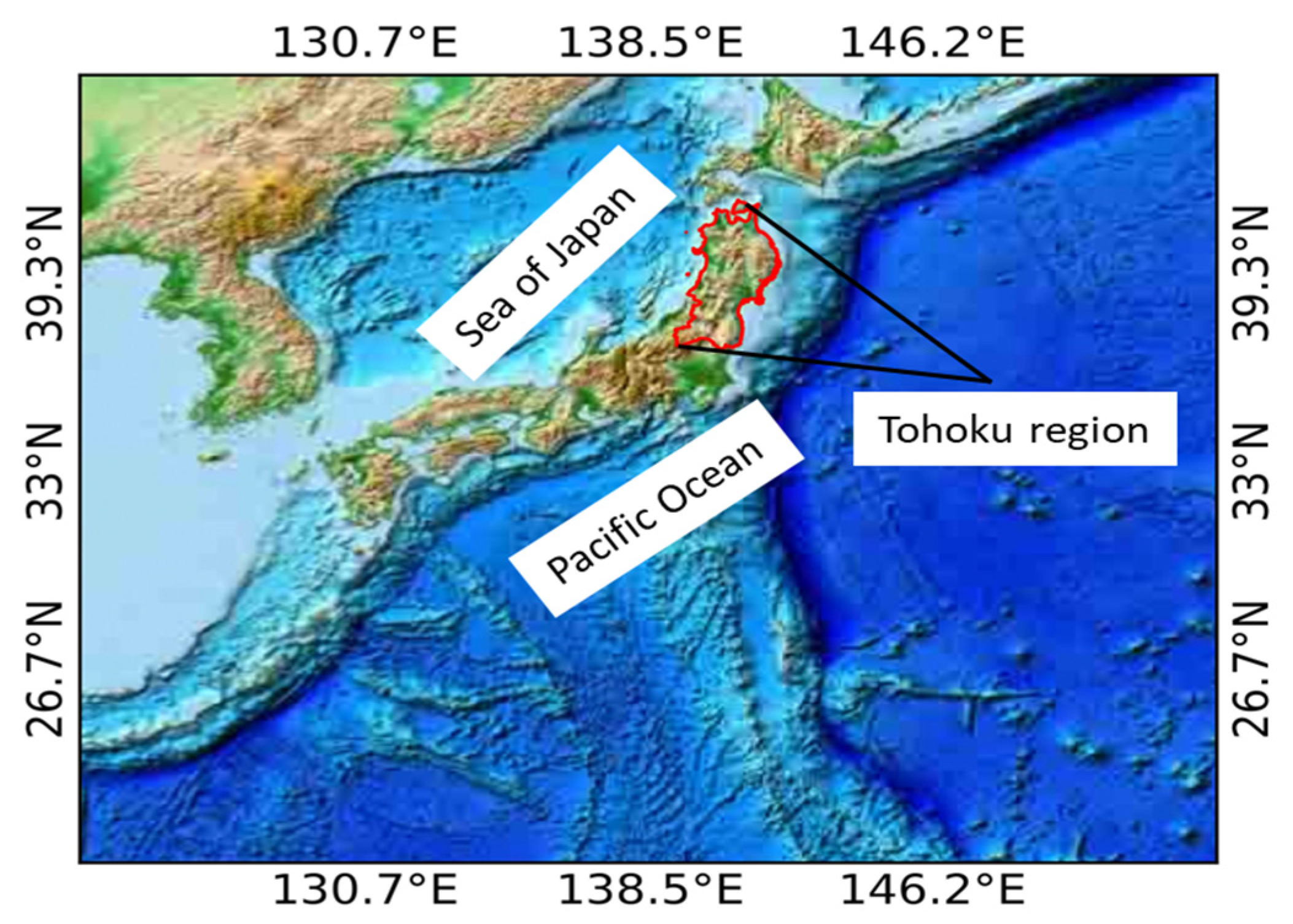
This research was implemented in the Tohoku region of Japan. The Ōu Mountains run through north to south in the middle of the region separating eastern (Pacific Ocean) and the western (Sea of Japan) sides of the region. Under the Köppen climate classification system, this region falls in a humid continental climate (Dfa) characterized by warm, short summers and long, cold winters; and a humid subtropical climate (Cfa) characterized by warm, wet summers, and cool, dry winters. The location map of the study area is shown in Figure 1.
It is a suitable area for the implementation of community-level vegetation classification systems because of the diversity of plant communities occurring in the region characterized by wider variations of both altitudinal and latitudinal ranges. The altitudinal variations differ from seashore to alpine regions, constituting three typical forest zones corresponding to temperature gradients, evergreen broad-leaved forests (Camellia japonica, Quercus glauca, etc.) distributed in the lower belt of warm temperate zone, deciduous broad-leaved forests (Fagus crenata, Quercus serrata, etc.) distributed in the cool temperate zone, and evergreen coniferous forests (Tsuga diversifolia, Thujopsis dolabrata, etc.) distributed in the subalpine zone.
2.2. DSPE Classification System
In the Dominant Species-Physiognomy-Ecological (DSPE) classification system, plant ecological communities are defined with the inference of Dominant Species, Physiognomy and shared Ecological conditions. The criteria of patch size have been used to standardize the selection of DSPE communities in the current research. The plant ecological communities usually forming larger than 100 × 100 m patch size for matrix patches (e.g., Abies firma Ecf, Fagus crenata Dbf, Betula ermanii Dbf) or larger than 30 × 100 m patch size for linear patches (e.g., Salix spp. Dbf, Pterocarya rhoifolia Dbf, Juglans mandshurica Dbf) were extracted as the dominant communities. In contrast to the minimum patch size of 30 × 30 m used in the previous analysis [24], the communities with smaller than 100 × 100 m or 30 × 100 m patch sizes were excluded in the current research. The criteria of minimum patch size determine the number of dominant plant communities enumerated and analyzed in the given area of interest. The list of DSPE communities enumerated and standardized for the current research has been shown in Table 1. The inferences used for defining the DSPE communities along with higher DGPE communities have also been described in Table 1.
As shown in Table 1, in the DSPE system, all forest communities have been classified into dominant species-physiognomy level. However, most of the herbaceous communities have been classified into physiognomy-ecological level. It is difficult to identify well-formed patches of the herbaceous communities at dominant species level. Rather, they can be identified effortlessly at physiognomy-ecological levels such as Coastal Hb, Open-space Hb, and Alpine Hb. Therefore, almost all herbaceous communities were classified into physiognomy-ecological level except the Miscanthus sinensis Dhb community forming distinct patches. Similarly, some shrub communities have been aggregated into dominant physiognomy-ecological level, such as Alpine Sb and Coastal Sb. However, most of the shrub communities have been classified into species-physiognomy level, such as Rhododendron spp. Esb, Salix spp. Dsb, and Sasa spp. Esb.
In the DSPE system, several species (spp.) of the same genus have been combined together for some forest communities. The combination of several species together depends on two criteria. First, whether the community forms a large enough patch (100 × 100 m for matrix patches or 30 × 100 for linear patches) at dominant species level or when several species (spp.) within the same genus are mixed together. For example, Salix spp. Dbf community, consisting of several Salix species in cool temperate ecosystems, or Quercus spp. Ebf community, consisting of several Quercus species in warm temperate ecosystems. Second, whether all species-level patches formed at distant places can be differentiated from satellite images satisfactorily or not. In the current research, several species were combined together if all species-level communities could not be classified with more than 50% kappa coefficient. For example, some Acer Dbf species could not be classified with more than 50% kappa coefficient due to similar phenology-spectral signatures. Therefore, several Acer species were combined together as Acer spp. Dbf community. Similarly, the same criteria were used to define shrub communities, for example Sasa spp. Esb and Rhododendron spp. Esb communities. In the DSPE system, mixed communities in ecotones with more than one dominant species can be combined together, such as the Abies sachalinensis Ecf–Quercus crispula Dbf community. In addition, different communities with similar phenology-spectral signatures can be combined together, such as Cryptomeria japonica Ecf–Chamaecyparis obtusa Ecf to minimize misclassification across similar dominant species. In the current research, multiple strata are incorporated for the communities, having distinct phenology-spectral signatures due to physiognomic variations between upper deciduous broadleaf trees and lower evergreen species. For example, Fagus spp. Dbf–Sasa spp. Esb. In the DGPE system, although plant communities with a single dominant species were also designated into genus-level only, these communities can be identified obviously into the species-level. For example, Pinus Sb (in the DGPE system) means Pinus pumila Esb because of the lack of other shrubby Pinus species in the given study area. The usage of physiognomy symbol (e.g., Dbf, Dsb, Ebf) aids to distinguish same species with a different physiognomy, such as distinguishing Quercus crispula Dbf from Quercus crispula Dsb and Quercus spp. Ebf.
It should be noted that the DSPE system is a flexible classification system in which expansion of the physiognomic-ecological communities into species level, combination of several species (spp.) of the same genus together, or inclusion of lower-stratum species can be adjusted within the framework of the DSPE system developed in the current research based on prior knowledge of the plant ecological communities of the study area and types and characteristics of the available remote sensing images for the classification.
2.3. Preparation of Ground Truth Data
The phytosociological units of the study area available from the extant vegetation survey maps (http://gis.biodic.go.jp/webgis, accessed on 25 May 2017) and associated database were initially utilized for enumerating dominant plant species of the study area. With reference to extant vegetation survey maps and Google Earth images, ground truth data (geo-location points) belonging to dominant plant species were collected by local flora experts in the previous study [24]. Based on this ground truth data, more than 125 dominant plant species of the study area were classified from multi-temporal and multi-spectral satellite images [24]. Another study [26] further increased the ground truth data for community-level mapping of plant communities in the study area. The current research utilized the ground truth data collected in the previous studies [24,26] after standardizing the working definition of the DSPE communities, and some additions with reference to extant vegetation survey maps and Google Earth images. The ground truth data size varied from 600–2400 for each DSPE community, depending on its proportional aerial coverage.
2.4. Processing of Satellite Data
All Level-2A product images collected by Sentinel-2 mission satellites (Sentinel-2A and 2B) for the whole study area between 2019–2021 were acquired and processed. The Sentinel-2 mission satellites acquire optical imagery at high-spatial resolution (10–60 m) in visible, near infrared, and short-wave wavelengths [27]. The Level-2A product provides Bottom of Atmosphere reflectance images after atmospheric and topographic correction [28,29]. The Sentinel-2 images were processed for cloud masking and ten spectral bands (blue, green, red, red edge 1–3, near infrared, mid infrared, and shortwave infrared 1–2) were extracted. The satellite-based spectral data were composited by computing half-monthly median values, and 240 features were generated in total for the recurrent deep learning.
2.5. Deep Recurrent Learning
Deep recurrent learning based on the Long Short-Term Memory (LSTM) networks [30] was employed for the classification of plant (ecological) communities using multi-temporal Sentinel-2 images. The LSTM can learn tasks that require memories of a time series of events that happened earlier, and it has proven to be effective for modeling complex non-linear relationships [31]. The model architecture was composed of four LSTM layers with tanh activations followed by two fully connected (dense) layers, one with relu activation and another final layer with softmax activation to collect classifications. The bootstrap resampling method was implemented to report the confidence interval of the classification [32]. The bootstrap resampling was done 1000 times with 75% training and 25% testing data. The parameters and hyper-parameters of the model including number of layers, number of neurons, learning rate, number of epochs, and batch size were fine-tuned with reference to the accuracy metrics (F1-score and Kappa coefficient) calculated with test data. The accuracy obtained with 25% test data was collected for each bootstrap resampling, and the frequency of model runs yielding the test accuracies was reported.
3. Results
3.1. Performance of DSPE Classification
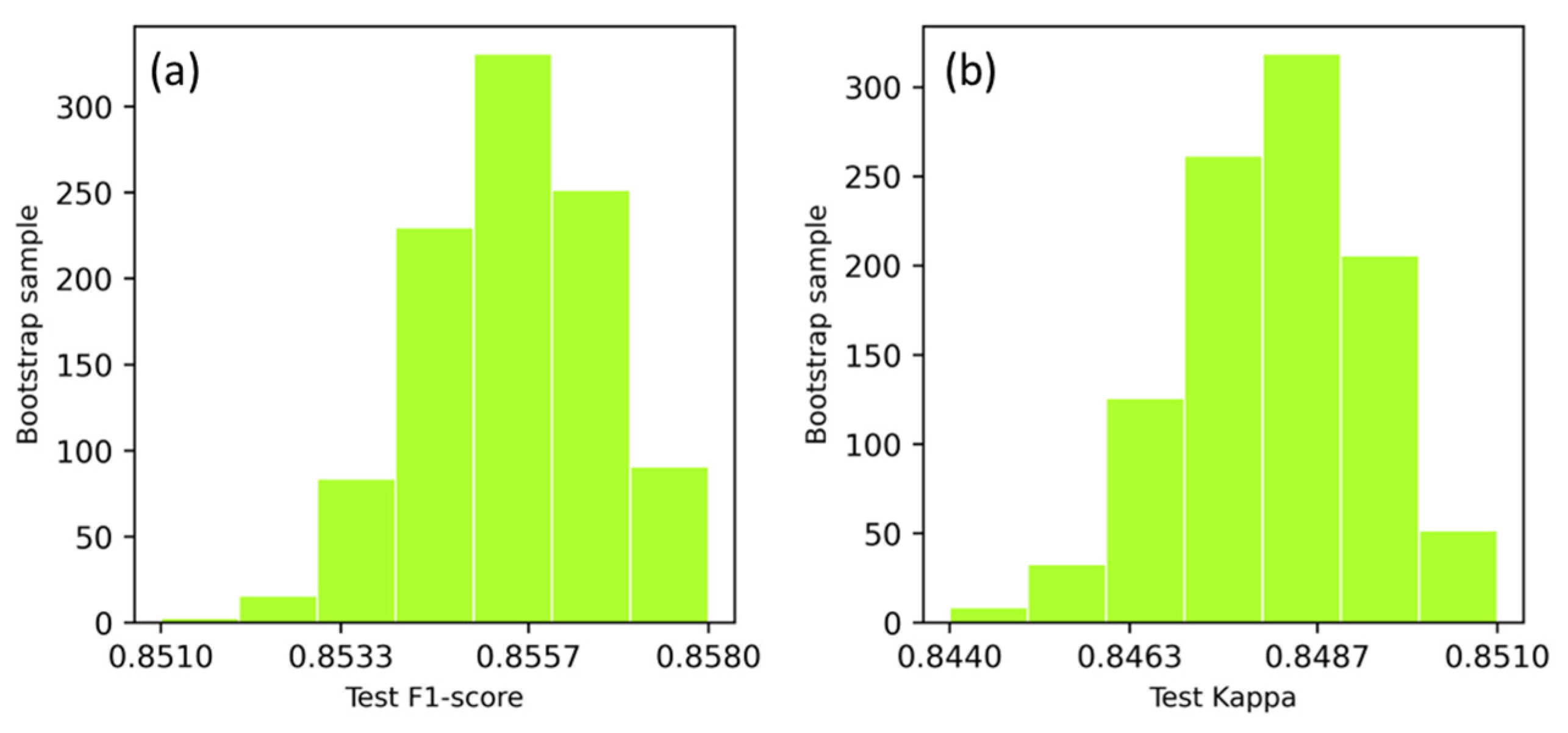
The DSPE classification accuracy in terms of F1-score and Kappa coefficient, obtained with 25% test data, was collected from 1000-run of bootstrap resampling, and the frequency of model runs resulting in test accuracies has been plotted in Figure 2. The test F1-score varied between 85.3–85.7% per 95% confidence interval, with an overall mean F1-score of 85.5%. The test Kappa coefficient varied between 84.5–85.0% per 95% confidence interval, with overall mean Kappa coefficient of 84.7%.
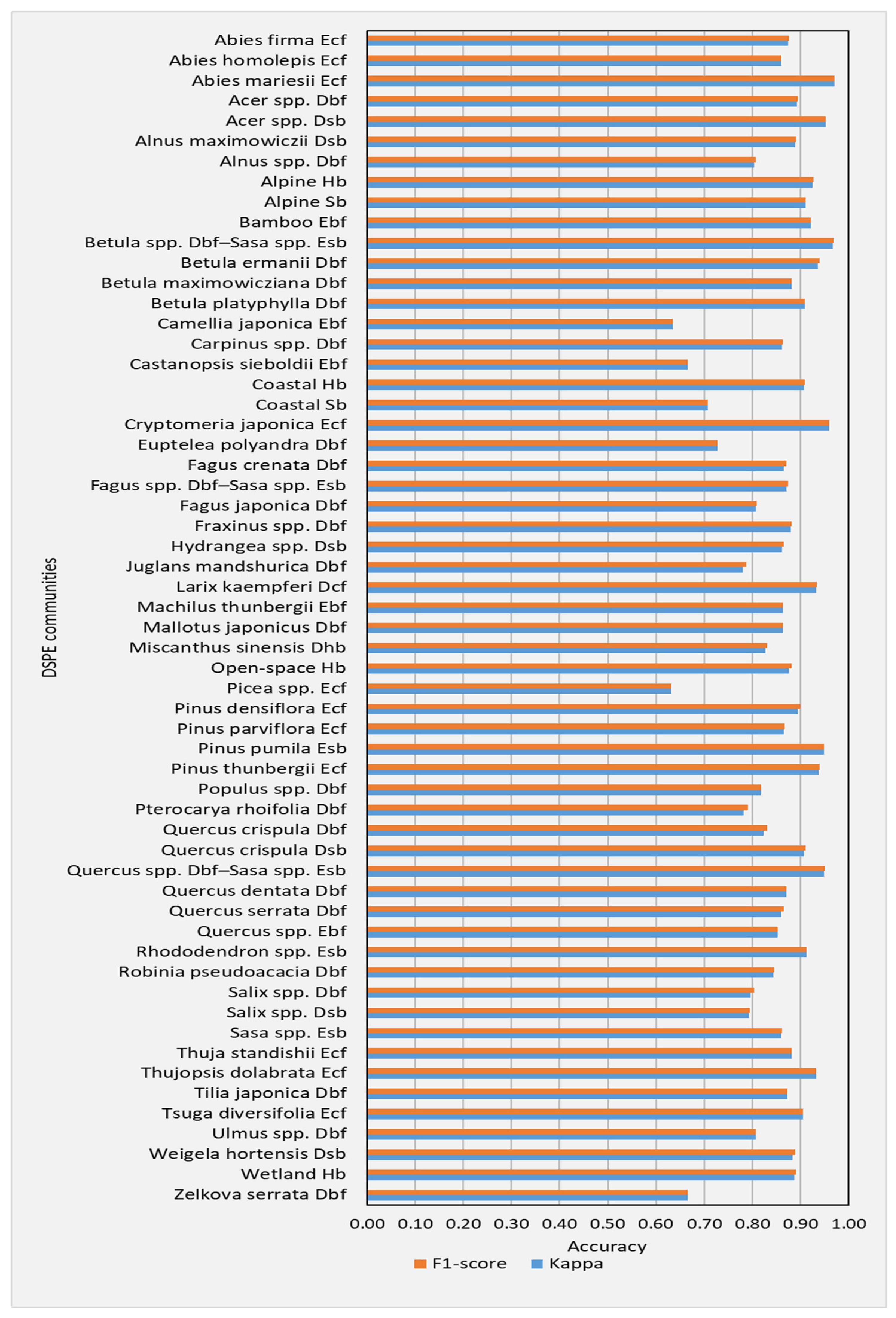
The class wise accuracies (F1-scores and Kappa coefficients) calculated with the test data for the classification of DSPE communities across 1000-run of bootstrap resampling were averaged, and the resulting averaged F1-score and Kappa coefficient values are shown in Figure 3.
3.2. Performance of DGPE Classification
The DGPE classification accuracy in terms of F1-score and Kappa coefficient, obtained with the test data, was collected from 1000-run of bootstrap resampling, and the frequency of model runs resulting in test accuracies was plotted in Figure 4. The test F1-score varied between 86.3–86.7% per 95% confidence interval, with overall mean of 86.5%. The Kappa coefficient varied between 85.5–86.0% per 95% confidence interval, with an overall mean Kappa coefficient of 85.7%.
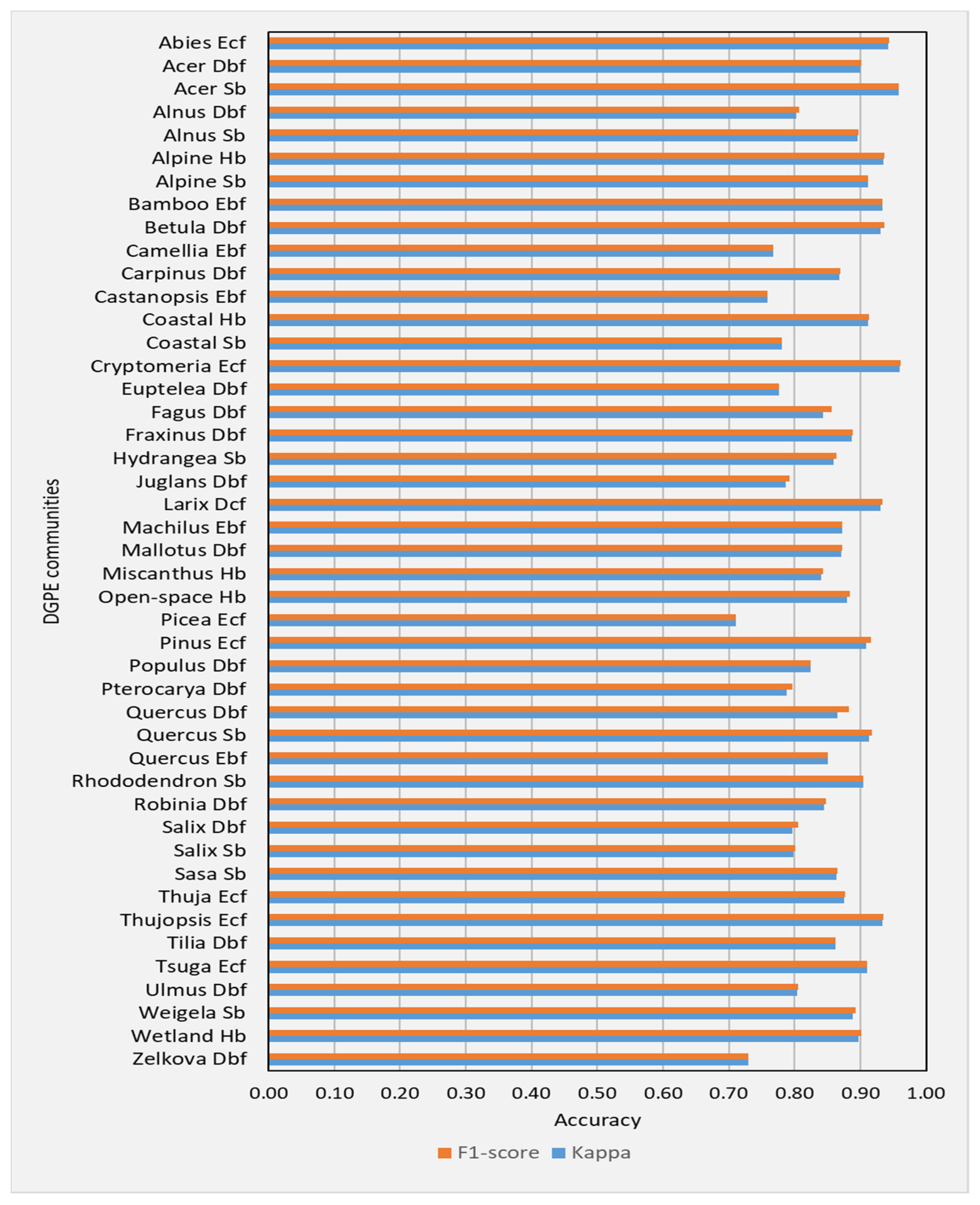
The class wise accuracies (F1-scores and Kappa coefficients) calculated with the test data for the classification of DGPE communities across 1000-run of bootstrap resampling were averaged, and the resulting averaged F1-score and Kappa coefficient values are shown in Figure 5.
The classification accuracy with deep recurrent neural networks across 1000-run of bootstrap resampling showed an overall 85.5% F1-score for the classification of 58 DSPE communities. Overall, there was a small difference in the classification between 58 DSPE communities (F1-score = 85.5%, Kappa coefficient = 84.7%) and 45 DGPE communities (F1-score = 86.5%, Kappa coefficient = 85.7%). The class wise accuracy analysis showed that all 58 DSPE were classified with more than 60% accuracy (F1-score and Kappa coefficient). However, more than 70% accuracy (F1-score and Kappa coefficient) was obtained for the classification of all 45 DGPE communities.
4. Discussion
The variations in vegetation zones and floristic composition under the influence of land use and climate change have brought enormous implications on landscape structure and ecological functioning in many regions of the world [33,34,35,36,37]. Survey and mapping of plant communities, as distinguishable patches of plant species formed within a geographical area, are not only relevant to quantitative analysis of vegetation-climate interactions, but also important for promoting environmental protection and management measures, particularly in an altering socio-economic context [38,39,40,41]. Contrary to a laborious field survey-based organization and delineation of plant communities, usage of remote sensing images has classified plant communities efficiently in many studies [42,43,44,45]. However, for large-scale applications and operational mapping, a right and suitable system is required for the organization of plant communities. In line with this, developing the DSPE classification system and evaluation of its potential for regional-scale differentiation of plant ecological communities is a timely and important contribution.
The floristic composition of a plant community in a geographical region occurs through the processes of adaptation, competition, and natural selection [46,47]. The pattern of a few abundant species, often referred to as a dominant species, and many rarer species are defining characteristics of communities worldwide [48]. Extinction of dominant species threatens much larger impacts on community and ecosystem processes compared with the extinction of rarer species [49,50]. Thus, the dominant species-based classification system presented in the research is vital to the study of ecological systems. The biodiversity conservation and management efforts require biological and ecological information at different levels from genes and species to communities, ecosystems, and landscapes [51]. In contrast to potential vegetation prediction approaches based on bio-climatic parameters at coarse spatial resolutions [52,53], the actual vegetation classification approaches carried out in the research can inform about the spatio-temporal ecological processes at fine spatial resolutions. The DSPE and DGPE classification systems are able to inform the floristic composition of the communities in contrast to the physiognomy-based systems [54]. Compared with a phytosociological system which usually deals with minimum mapping unit of 1 ha, e.g., [55], the DSPE and DGPE classification systems are also capable of individual crown level mapping with modern day ultra-resolution remote sensing images [56].
In recent years, the usage of artificial intelligence, particularly deep neural-networks, has gained momentum in ecological applications as a versatile technology specialized for big datasets [57,58,59,60]. Deep neural-networks learning has been reported as a powerful state-of-the-art technique for classification of multi-temporal satellite imagery [61] and utilized by many previous studies for the classification and mapping of vegetation using remote sensing images [62,63,64,65,66]. This research employed deep recurrent learning as an efficient classifier for dealing with time-series of the satellite data involved with the differentiation of regional-scale plant (ecological) communities. Previous research has described the robustness of the deep recurrent learning based on Long Short-Term Memory (LSTM) networks for the classification of time-series of the satellite data [67,68,69,70]. Since the phenology-spectral information is vital to the differentiation of plant ecological communities, the LSTM networks designed for dealing with the time-series of the data were effective. Nevertheless, some DSPE communities were misclassified pertaining to similar phenology-spectral signatures, especially among the evergreen broadleaf communities such as Camellia japonica Ebf, Quercus spp. Ebf, and Castanopsis sieboldii Ebf. Another large misclassification in deciduous broadleaf forests was found among the classification of Salix spp. Dbf, Euptelea polyandra Dbf, and Zelkova serrata Dbf. However, communities across the physiognomic differences were usually classified satisfactorily. When species-level information is not required, the DGPE system is still capable of distinguishing a wide variety of plant ecological communities, such as Quercus Ebf (warm temperate), Quercus Dbf (cool temperate), and Quercus Sb (alpine). It is expected that the classification of DSPE communities can be improved through the advancement of remote sensing technologies in the future. Previous research has also reported complexities associated with the classification of tree species from satellite imagery, particularly in heterogeneous landscapes [71,72]. Accuracy obtained in the current research is consistent with recent studies on the classification of ecological communities from satellite images. For example, Kluczek et al. [73] obtained an F1-score in the range of 76–90% for the classification of 13 mountain forest and non-forest plant communities. Similarly, another study by Martínez Prentice et al. [74] obtained 80% Kappa coefficient using Random Forests classifier in the classification of coastal wetlands. However, in contrast to these local-scale classifications, achieving 85.5% F1-score and 84.7% Kappa in the classification of 58 DSPE communities in the current research at a regional-scale is a significant contribution.
5. Conclusions
In this research, the DSPE classification system was developed for large-scale differentiation of plant ecological communities from remote sensing images. The performance of DSPE classification of plant ecological communities was compared to higher-level classification of DGPE communities by employing deep recurrent learning of multi-temporal and multi-spectral satellite images at 10 m spatial resolution at a regional scale. Although the differentiation of higher-level DGPE communities showed a slightly higher performance (F1-score = 86.5%, Kappa coefficient = 85.7%) than the differentiation of DSPE communities overall (F1-score = 85.5%, Kappa coefficient = 84.7%), the DSPE classification system has the capacity to differentiate most of the ecological communities into a dominant species level in contrast to the dominant genus-level differentiation of most of the communities by the DGPE system. Since all 58 DSPE communities were classified with more than 60% accuracy (in terms of F1-score and Kappa coefficient), the DSPE classification system was still found to be effective for the differentiation of plant ecological communities efficiently from satellite images. The DSPE and DGPE classification systems are expected to be useful for community-level vegetation mapping in other regions as well.
Funding
This research received no funding.
Institutional Review Board Statement
Not applicable.
Informed Consent Statement
Not applicable.
Data Availability Statement
Not applicable.
Acknowledgments
The vegetation survey maps were available from Biodiversity Center, Ministry of the Environment, Japan. Portion of the ground truth data was previously provided by the commissioned research of the Biodiversity Center of Japan and Asia Air Survey Co., Ltd., Japan. Keitarou Hara is appreciated for supporting field survey of plant communities. Author is grateful to anonymous reviewers and editors for the constructive comments and suggestions which were vital for designing the manuscript to this form.
Conflicts of Interest
The author declares no conflict of interest.
References
- Maarel, E. Vegetation Mapping: Vegetation Science in Need of a New Handbook. J. Veg. Sci. 1991, 2, 421–424. [Google Scholar] [CrossRef]
- Mucina, L. Classification of Vegetation: Past, Present and Future. J. Veg. Sci. 1997, 8, 751–760. [Google Scholar] [CrossRef]
- Küchler, A.W.; Zonneveld, I.S. Vegetation Mapping; Springer: Dordrecht, The Netherlands, 1988; ISBN 978-94-009-3083-4. [Google Scholar]
- Grossman, D.; Faber-Langendoen, D.; Weakley, A.; Anderson, M.; Bourgeron, P.; Crawford, R.; Goodin, K.; Landaal, S.; Metzler, K.; Patterson, K. International Classification of Ecological Communities: Terrestrial Vegetation of the United States; The Nature Conservancy: Arlington County, VA, USA, 1998. [Google Scholar]
- Gleason, H.A. The Individualistic Concept of the Plant Association. Bull. Torrey Bot. Club 1926, 53, 7. [Google Scholar] [CrossRef]
- Moravec, J. Influences of the Individualistic Concept of Vegetation on Syntaxonomy. Vegetatio 1989, 81, 29–39. [Google Scholar] [CrossRef]
- Collins, S.L.; Glenn, S.M.; Roberts, D.W. The Hierarchical Continuum Concept. J. Veg. Sci. 1993, 4, 149–156. [Google Scholar] [CrossRef]
- Clements, F.E. Plant Succession: An Analysis of the Development of Vegetation; Carnegie Institution of Washington: Washington, DC, USA, 1916. [Google Scholar]
- McIntosh, R.P. The Continuum Concept of Vegetation. Bot. Rev. 1967, 33, 130–187. [Google Scholar] [CrossRef]
- Austin, M.P. Continuum Concept, Ordination Methods, and Niche Theory. Annu. Rev. Ecol. Syst. 1985, 16, 39–61. [Google Scholar] [CrossRef]
- Mitchell, R.M.; Bakker, J.D.; Vincent, J.B.; Davies, G.M. Relative Importance of Abiotic, Biotic, and Disturbance Drivers of Plant Community Structure in the Sagebrush Steppe. Ecol. Appl. 2017, 27, 756–768. [Google Scholar] [CrossRef]
- Whittaker, R.H. Classification of Plant Communities; Springer: Dordrecht, The Netherlands, 1980; ISBN 978-94-009-9183-5. [Google Scholar]
- McIntosh, R.P. Concept and Terminology of Homogeneity and Heterogeneity in Ecology. In Ecological Heterogeneity; Kolasa, J., Pickett, S.T.A., Eds.; Ecological Studies; Springer: New York, NY, USA, 1991; Volume 86, pp. 24–46. ISBN 978-1-4612-7781-1. [Google Scholar]
- Bedward, M.; Keith, D.A.; Pressey, R.L. Homogeneity Analysis: Assessing the Utility of Classifications and Maps of Natural Resources. Austral. Ecol. 1992, 17, 133–139. [Google Scholar] [CrossRef]
- Feagin, R.A. Heterogeneity versus Homogeneity: A Conceptual and Mathematical Theory in Terms of Scale-Invariant and Scale-Covariant Distributions. Ecol. Complex. 2005, 2, 339–356. [Google Scholar] [CrossRef]
- Köppen, W. Das Geographische System der Klimate. Available online: http://koeppen-geiger.vu-wien.ac.at/pdf/Koppen_1936.pdf (accessed on 20 March 2022).
- Bailey, R.G. Ecosystem Geography: From Ecoregions to Sites, 2nd ed.; Springer: New York, NY, USA, 2009; ISBN 978-0-387-89515-4. [Google Scholar]
- Metzger, M.J.; Bunce, R.G.H.; Jongman, R.H.G.; Sayre, R.; Trabucco, A.; Zomer, R. A High-Resolution Bioclimate Map of the World: A Unifying Framework for Global Biodiversity Research and Monitoring. Glob. Ecol. Biogeogr. 2013, 22, 630–638. [Google Scholar] [CrossRef]
- Küchler, A.W. A Physiognomic Classification of Vegetation. Ann. Assoc. Am. Geogr. 1949, 39, 201–210. [Google Scholar] [CrossRef]
- Beard, J.S. The Physiognomic Approach. In Classification of Plant Communities; Whittaker, R.H., Ed.; Springer: Dordrecht, The Netherlands, 1978; pp. 33–64. ISBN 978-94-009-9183-5. [Google Scholar]
- Braun-Blanquet, J. Pflanzensoziologie; Springer: Vienna, Austria, 1964; ISBN 978-3-7091-8111-9. [Google Scholar]
- Westhoff, V.; Van Der Maarel, E. The Braun-Blanquet Approach. In Classification of Plant Communities; Springer: New York, NY, USA, 1978; pp. 287–399. [Google Scholar]
- Gaston, K.J. Valuing Common Species. Science 2010, 327, 154–155. [Google Scholar] [CrossRef]
- Sharma, R.C. Genus-Physiognomy-Ecosystem (GPE) System for Satellite-Based Classification of Plant Communities. Ecologies 2021, 2, 203–213. [Google Scholar] [CrossRef]
- Sharma, R.C. Countrywide Mapping of Plant Ecological Communities with 101 Legends Including Land Cover Types for the First Time at 10 m Resolution through Convolutional Learning of Satellite Images. Appl. Sci. 2022, 12, 7125. [Google Scholar] [CrossRef]
- Sharma, R.C.; Hirayama, H.; Yasuda, M.; Asai, M.; Hara, K. Classification and Mapping of Plant Communities Using Multi-Temporal and Multi-Spectral Satellite Images. J. Geogr. Geol. 2022, 14, 43. [Google Scholar] [CrossRef]
- Drusch, M.; Del Bello, U.; Carlier, S.; Colin, O.; Fernandez, V.; Gascon, F.; Hoersch, B.; Isola, C.; Laberinti, P.; Martimort, P.; et al. Sentinel-2: ESA’s Optical High-Resolution Mission for GMES Operational Services. Remote Sens. Environ. 2012, 120, 25–36. [Google Scholar] [CrossRef]
- Mayer, B.; Kylling, A. Technical Note: The LibRadtran Software Package for Radiative Transfer Calculations—Description and Examples of Use. Atmos. Chem. Phys. 2005, 5, 1855–1877. [Google Scholar] [CrossRef]
- Richter, R.; Schläpfer, D. Atmospheric/Topographic Correction for Satellite Imagery. Available online: https://www.rese.ch/pdf/atcor3_manual.pdf (accessed on 20 March 2022).
- Hochreiter, S.; Schmidhuber, J. Long Short-Term Memory. Neural Comput. 1997, 9, 1735–1780. [Google Scholar] [CrossRef] [PubMed]
- Schmidhuber, J. Deep Learning in Neural Networks: An Overview. Neural Netw. 2015, 61, 85–117. [Google Scholar] [CrossRef]
- Dixon, P.M. Bootstrap Resampling. In Encyclopedia of Environmetrics; El-Shaarawi, A.H., Piegorsch, W.W., Eds.; Wiley: Hoboken, NJ, USA, 2001; ISBN 978-0-471-89997-6. [Google Scholar]
- Aggemyr, E.; Cousins, S.A.O. Landscape Structure and Land Use History Influence Changes in Island Plant Composition after 100 Years: Revisiting 27 Islands after 100 Years. J. Biogeogr. 2012, 39, 1645–1656. [Google Scholar] [CrossRef]
- Franklin, J.; Serra-Diaz, J.M.; Syphard, A.D.; Regan, H.M. Global Change and Terrestrial Plant Community Dynamics. Proc. Natl. Acad. Sci. USA 2016, 113, 3725–3734. [Google Scholar] [CrossRef]
- Chen, C.; Wu, S.; Meurk, C.D.; Ma, M.; Zhao, J.; Mingquan, L.; Tong, X. Effects of Local and Landscape Factors on Exotic Vegetation in the Riparian Zone of a Regulated River: Implications for Reservoir Conservation. Landsc. Urban Plan. 2017, 157, 45–55. [Google Scholar] [CrossRef]
- Prokopová, M.; Salvati, L.; Egidi, G.; Cudlín, O.; Včeláková, R.; Plch, R.; Cudlín, P. Envisioning Present and Future Land-Use Change under Varying Ecological Regimes and Their Influence on Landscape Stability. Sustainability 2019, 11, 4654. [Google Scholar] [CrossRef]
- Afuye, G.A.; Kalumba, A.M.; Busayo, E.T.; Orimoloye, I.R. A Bibliometric Review of Vegetation Response to Climate Change. Env. Sci. Pollut. Res. 2022, 29, 18578–18590. [Google Scholar] [CrossRef]
- Zeng, N.; Neelin, J.D. The Role of Vegetation–Climate Interaction and Interannual Variability in Shaping the African Savanna. J. Clim. 2000, 13, 2665–2670. [Google Scholar] [CrossRef]
- Götzenberger, L.; de Bello, F.; Bråthen, K.A.; Davison, J.; Dubuis, A.; Guisan, A.; Lepš, J.; Lindborg, R.; Moora, M.; Pärtel, M.; et al. Ecological Assembly Rules in Plant Communities-Approaches, Patterns and Prospects. Biol. Rev. 2012, 87, 111–127. [Google Scholar] [CrossRef]
- Cannone, N.; Pignatti, S. Ecological Responses of Plant Species and Communities to Climate Warming: Upward Shift or Range Filling Processes? Clim. Chang. 2014, 123, 201–214. [Google Scholar] [CrossRef]
- Diao, C.; Liu, Y.; Zhao, L.; Zhuo, G.; Zhang, Y. Regional-Scale Vegetation-Climate Interactions on the Qinghai-Tibet Plateau. Ecol. Inform. 2021, 65, 101413. [Google Scholar] [CrossRef]
- Gould, W. Remote sensing of vegetation, plant species richness, and regional biodiversity hotspots. Ecol. Appl. 2000, 10, 1861–1870. [Google Scholar] [CrossRef]
- Mathieu, R.; Aryal, J.; Chong, A. Object-Based Classification of Ikonos Imagery for Mapping Large-Scale Vegetation Communities in Urban Areas. Sensors 2007, 7, 2860–2880. [Google Scholar] [CrossRef] [PubMed]
- Xie, Y.; Sha, Z.; Yu, M. Remote Sensing Imagery in Vegetation Mapping: A Review. J. Plant Ecol. 2008, 1, 9–23. [Google Scholar] [CrossRef]
- He, K.S.; Rocchini, D.; Neteler, M.; Nagendra, H. Benefits of Hyperspectral Remote Sensing for Tracking Plant Invasions: Plant Invasion and Hyperspectral Remote Sensing. Divers. Distrib. 2011, 17, 381–392. [Google Scholar] [CrossRef]
- Watt, A.S. Pattern and Process in the Plant Community. J. Ecol. 1947, 35, 1. [Google Scholar] [CrossRef]
- Cullum, C.; Rogers, K.H.; Brierley, G.; Witkowski, E.T.F. Ecological Classification and Mapping for Landscape Management and Science: Foundations for the Description of Patterns and Processes. Prog. Phys. Geogr. Earth Environ. 2016, 40, 38–65. [Google Scholar] [CrossRef]
- Avolio, M.L.; Forrestel, E.J.; Chang, C.C.; La Pierre, K.J.; Burghardt, K.T.; Smith, M.D. Demystifying Dominant Species. New Phytol. 2019, 223, 1106–1126. [Google Scholar] [CrossRef] [PubMed]
- Smith, M.D.; Knapp, A.K. Dominant Species Maintain Ecosystem Function with Non-Random Species Loss. Ecol. Lett. 2003, 6, 509–517. [Google Scholar] [CrossRef]
- Winfree, R.; Fox, J.W.; Williams, N.M.; Reilly, J.R.; Cariveau, D.P. Abundance of Common Species, Not Species Richness, Drives Delivery of a Real-World Ecosystem Service. Ecol. Lett. 2015, 18, 626–635. [Google Scholar] [CrossRef] [PubMed]
- Perino, A.; Pereira, H.M.; Felipe-Lucia, M.; Kim, H.; Kühl, H.S.; Marselle, M.R.; Meya, J.N.; Meyer, C.; Navarro, L.M.; van Klink, R.; et al. Biodiversity Post-2020: Closing the Gap between Global Targets and National-level Implementation. Conserv. Lett. 2022, 15, e12848. [Google Scholar] [CrossRef]
- Hengl, T.; Walsh, M.G.; Sanderman, J.; Wheeler, I.; Harrison, S.P.; Prentice, I.C. Global Mapping of Potential Natural Vegetation: An Assessment of Machine Learning Algorithms for Estimating Land Potential. PeerJ 2018, 6, e5457. [Google Scholar] [CrossRef]
- Sato, H.; Ise, T. Predicting Global Terrestrial Biomes with the LeNet Convolutional Neural Network. Geosci. Model Dev. 2022, 15, 3121–3132. [Google Scholar] [CrossRef]
- Ellenberg, H.; Mueller-Dombois, D. Tentative Physiognomic-Ecological Classification of Plant Formations of the Earth. Available online: https://doi.org/10.5169/SEALS-377650 (accessed on 10 March 2022).
- Noriyuki, M.; Kondo, H.; Shitara, T.; Yoshikawa, M.; Hoshino, Y. A New Formal Classification for Japanese Forest Vegetation Based on Traditional Phytosociological Concepts. Appl. Veg. Sci. 2021, 24, e12611. [Google Scholar] [CrossRef]
- Sharma, R.C. An Ultra-Resolution Features Extraction Suite for Community-Level Vegetation Differentiation and Mapping at a Sub-Meter Resolution. Remote Sens. 2022, 14, 3145. [Google Scholar] [CrossRef]
- Özesmi, S.L.; Tan, C.O.; Özesmi, U. Methodological Issues in Building, Training, and Testing Artificial Neural Networks in Ecological Applications. Ecol. Model. 2006, 195, 83–93. [Google Scholar] [CrossRef]
- Brodrick, P.G.; Davies, A.B.; Asner, G.P. Uncovering Ecological Patterns with Convolutional Neural Networks. Trends Ecol. Evol. 2019, 34, 734–745. [Google Scholar] [CrossRef] [PubMed]
- Christin, S.; Hervet, É.; Lecomte, N. Applications for Deep Learning in Ecology. Methods Ecol. Evol. 2019, 10, 1632–1644. [Google Scholar] [CrossRef]
- Ryo, M.; Angelov, B.; Mammola, S.; Kass, J.M.; Benito, B.M.; Hartig, F. Explainable Artificial Intelligence Enhances the Ecological Interpretability of Black-box Species Distribution Models. Ecography 2021, 44, 199–205. [Google Scholar] [CrossRef]
- Kussul, N.; Lavreniuk, M.; Skakun, S.; Shelestov, A. Deep Learning Classification of Land Cover and Crop Types Using Remote Sensing Data. IEEE Geosci. Remote Sens. Lett. 2017, 14, 778–782. [Google Scholar] [CrossRef]
- Carpenter, G.A.; Gopal, S.; Macomber, S.; Martens, S.; Woodcock, C.E.; Franklin, J. A Neural Network Method for Efficient Vegetation Mapping. Remote Sens. Environ. 1999, 70, 326–338. [Google Scholar] [CrossRef]
- Campos-Taberner, M.; García-Haro, F.J.; Martínez, B.; Izquierdo-Verdiguier, E.; Atzberger, C.; Camps-Valls, G.; Gilabert, M.A. Understanding Deep Learning in Land Use Classification Based on Sentinel-2 Time Series. Sci. Rep. 2020, 10, 17188. [Google Scholar] [CrossRef] [PubMed]
- Zhan, Z.; Zhang, X.; Liu, Y.; Sun, X.; Pang, C.; Zhao, C. Vegetation Land Use/Land Cover Extraction from High-Resolution Satellite Images Based on Adaptive Context Inference. IEEE Access 2020, 8, 21036–21051. [Google Scholar] [CrossRef]
- Bakhti, K.; El Amin Larabi, M. Comparing Deep Recurrent Learning and Convolutional Learning for Multi-Temporal Vegetation Classification. In Proceedings of the 2021 IEEE International Geoscience and Remote Sensing Symposium IGARSS, Brussels, Belgium, 11–16 July 2021; pp. 4392–4395. [Google Scholar]
- Neves, A.K.; Körting, T.S.; Fonseca, L.M.G.; Soares, A.R.; Girolamo-Neto, C.D.; Heipke, C. Hierarchical Mapping of Brazilian Savanna (Cerrado) Physiognomies Based on Deep Learning. J. Appl. Rem. Sens. 2021, 15, 044504. [Google Scholar] [CrossRef]
- Ienco, D.; Gaetano, R.; Dupaquier, C.; Maurel, P. Land Cover Classification via Multitemporal Spatial Data by Deep Recurrent Neural Networks. IEEE Geosci. Remote Sens. Lett. 2017, 14, 1685–1689. [Google Scholar] [CrossRef]
- Lakhal, M.I.; Çevikalp, H.; Escalera, S.; Ofli, F. Recurrent Neural Networks for Remote Sensing Image Classification. IET Comput. Vis. 2018, 12, 1040–1045. [Google Scholar] [CrossRef]
- Wang, H.; Zhao, X.; Zhang, X.; Wu, D.; Du, X. Long Time Series Land Cover Classification in China from 1982 to 2015 Based on Bi-LSTM Deep Learning. Remote Sens. 2019, 11, 1639. [Google Scholar] [CrossRef]
- Sun, Z.; Di, L.; Fang, H. Using Long Short-Term Memory Recurrent Neural Network in Land Cover Classification on Landsat and Cropland Data Layer Time Series. Int. J. Remote Sens. 2019, 40, 593–614. [Google Scholar] [CrossRef]
- Mishra, A.P.; Rai, I.D.; Pangtey, D.; Padalia, H. Vegetation Characterization at Community Level Using Sentinel-2 Satellite Data and Random Forest Classifier in Western Himalayan Foothills, Uttarakhand. J. Indian Soc. Remote Sens. 2021, 49, 759–771. [Google Scholar] [CrossRef]
- Adagbasa, E.G.; Adelabu, S.A.; Okello, T.W. Application of Deep Learning with Stratified K-Fold for Vegetation Species Discrimation in a Protected Mountainous Region Using Sentinel-2 Image. Geocarto Int. 2022, 37, 142–162. [Google Scholar] [CrossRef]
- Kluczek, M.; Zagajewski, B.; Kycko, M. Airborne HySpex Hyperspectral Versus Multitemporal Sentinel-2 Images for Mountain Plant Communities Mapping. Remote Sens. 2022, 14, 1209. [Google Scholar] [CrossRef]
- Martínez Prentice, R.; Villoslada Peciña, M.; Ward, R.D.; Bergamo, T.F.; Joyce, C.B.; Sepp, K. Machine Learning Classification and Accuracy Assessment from High-Resolution Images of Coastal Wetlands. Remote Sens. 2021, 13, 3669. [Google Scholar] [CrossRef]
Figure 1.
Location map of the study area.

Figure 2.
Distribution of test accuracies with 1000-run of bootstrap resampling for the classification of DSPE communities using F1-score (a) and Kappa coefficient (b).
Figure 2.
Distribution of test accuracies with 1000-run of bootstrap resampling for the classification of DSPE communities using F1-score (a) and Kappa coefficient (b).

Figure 3.
Class wise mean F1-score and Kappa coefficient values calculated for the classification of DSPE communities across 1000-run of bootstrap resampling.
Figure 3.
Class wise mean F1-score and Kappa coefficient values calculated for the classification of DSPE communities across 1000-run of bootstrap resampling.

Figure 4.
Distribution of test accuracies with 1000-run of bootstrap resampling for the classification of DGPE communities using F1-score (a) and Kappa coefficient (b).
Figure 4.
Distribution of test accuracies with 1000-run of bootstrap resampling for the classification of DGPE communities using F1-score (a) and Kappa coefficient (b).
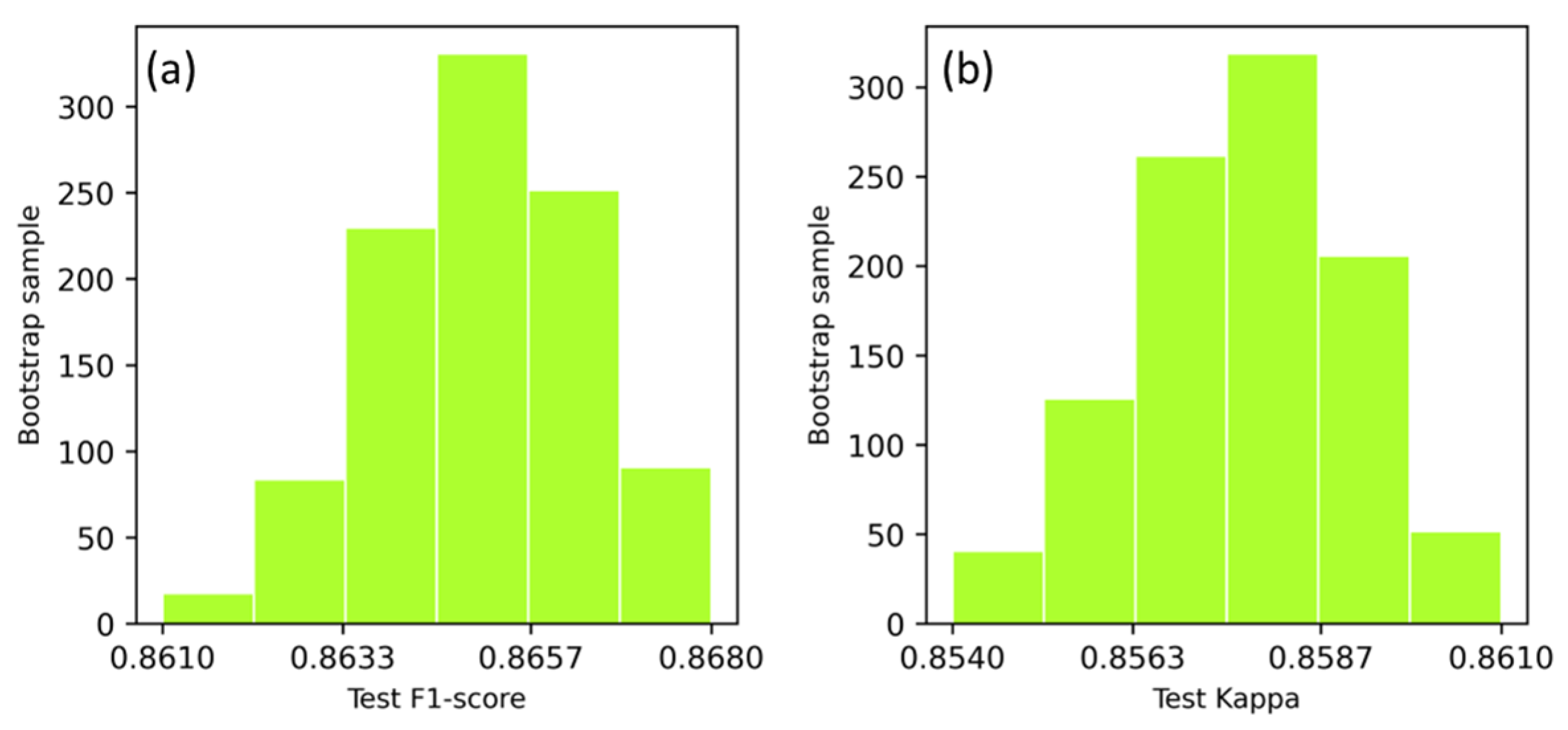
Figure 5.
Class wise mean F1-score and Kappa coefficient values calculated for the classification of DGPE communities across 1000-run of bootstrap resampling.
Figure 5.
Class wise mean F1-score and Kappa coefficient values calculated for the classification of DGPE communities across 1000-run of bootstrap resampling.


Table 1.
List of DSPE communities of the study area and the inferences used for defining them.
| DSPE | Inference | DGPE |
|---|---|---|
| Species-Physiognomy | Abies Ecf |
| Species-Physiognomy | Abies Ecf |
| Species-Physiognomy | Abies Ecf |
| Species-Physiognomy | Acer Dbf |
| Species-Physiognomy | Acer Sb |
| Species-Physiognomy | Alnus Dbf |
| Species-Physiognomy | Alnus Dsb |
| Physiognomy-Ecological | Alpine Hb |
| Physiognomy-Ecological | Alpine Sb |
| Physiognomy-Ecological | Bamboo Ebf |
| Species-Physiognomy | Betula Dbf |
| Species-Physiognomy | Betula Dbf |
| Species-Physiognomy | Betula Dbf |
| Species-Physiognomy (Multi strata) | Betula Dbf |
| Species-Physiognomy | Camellia Ebf |
| Species-Physiognomy | Carpinus Dbf |
| Species-Physiognomy | Castanopsis Ebf |
| Physiognomy-Ecological | Coastal Hb |
| Physiognomy-Ecological | Coastal Sb |
| Species-Physiognomy | Cryptomeria Ecf |
| Species-Physiognomy (Multi strata) | Fagus Dbf |
| Species-Physiognomy | Euptelea Dbf |
| Species-Physiognomy | Fagus Dbf |
| Species-Physiognomy | Fagus Dbf |
| Species-Physiognomy | Fraxinus Dbf |
| Species-Physiognomy | Hydrangea Sb |
| Species-Physiognomy | Juglans Dbf |
| Species-Physiognomy | Larix Dcf |
| Species-Physiognomy | Machilus Ebf |
| Species-Physiognomy | Mallotus Dbf |
| Species-Physiognomy | Miscanthus Hb |
| Physiognomy-Ecological | Open-space Hb |
| Species-Physiognomy (Multi strata) | Quercus Dbf |
| Species-Physiognomy | Picea Ecf |
| Species-Physiognomy | Pinus Ecf |
| Species-Physiognomy | Pinus Ecf |
| Species-Physiognomy | Pinus Sb |
| Species-Physiognomy | Pinus Ecf |
| Species-Physiognomy | Populus Dbf |
| Species-Physiognomy | Pterocarya Dbf |
| Species-Physiognomy | Quercus Dbf |
| Species-Physiognomy | Quercus Dbf |
| Species-Physiognomy | Quercus Ebf |
| Species-Physiognomy | Quercus Dbf |
| Species-Physiognomy | Quercus Sb |
| Species-Physiognomy | Rhododendron Sb |
| Species-Physiognomy | Robinia Dbf |
| Species-Physiognomy | Salix Dbf |
| Species-Physiognomy | Salix Sb |
| Species-Physiognomy | Sasa Sb |
| Species-Physiognomy | Thuja Ecf |
| Species-Physiognomy | Thujopsis Ecf |
| Species-Physiognomy | Tilia Dbf |
| Species-Physiognomy | Tsuga Ecf |
| Species-Physiognomy | Ulmus Dbf |
| Species-Physiognomy | Weigela Sb |
| Physiognomy-Ecological | Wetland Hb |
| Species-Physiognomy | Zelkova Dbf |
Ebf: Evergreen broadleaf forest; Dbf: Deciduous broadleaf forest; Dcf: Deciduous conifer forest. Ecf: Evergreen conifer forest; Esb: Evergreen shrub; Dsb: Deciduous shrub; Dhb: Deciduous herb; Hb: Herb; Sb: Shrub; spp.: Several species.
Publisher’s Note: MDPI stays neutral with regard to jurisdictional claims in published maps and institutional affiliations. |
© 2022 by the author. Licensee MDPI, Basel, Switzerland. This article is an open access article distributed under the terms and conditions of the Creative Commons Attribution (CC BY) license (https://creativecommons.org/licenses/by/4.0/).
Share and Cite
MDPI and ACS Style
Sharma, R.C. Dominant Species-Physiognomy-Ecological (DSPE) System for the Classification of Plant Ecological Communities from Remote Sensing Images. Ecologies 2022, 3, 323-335. https://doi.org/10.3390/ecologies3030025
AMA Style
Sharma RC. Dominant Species-Physiognomy-Ecological (DSPE) System for the Classification of Plant Ecological Communities from Remote Sensing Images. Ecologies. 2022; 3(3):323-335. https://doi.org/10.3390/ecologies3030025
Chicago/Turabian StyleSharma, Ram C. 2022. "Dominant Species-Physiognomy-Ecological (DSPE) System for the Classification of Plant Ecological Communities from Remote Sensing Images" Ecologies 3, no. 3: 323-335. https://doi.org/10.3390/ecologies3030025