No Country for Old Frameworks? Vertex Models and Their Ongoing Reinvention to Study Tissue Dynamics

Abstract

Vertex models have become essential tools for understanding tissue morphogenesis by simulating the mechanical and geometric properties of cells in various biological systems. These models represent cells as polygons or polyhedra, capturing cellular interactions such as adhesion, tension, and force generation. This review explores the ongoing evolution of computational vertex models, highlighting their application to complex tissue dynamics, including organoid development, wound healing, and cancer metastasis. We examine different energy formulations used in vertex models, which account for mechanical forces such as surface tension, volume conservation, and intercellular adhesion. Additionally, this review discusses the challenges of expanding traditional 2D models to 3D structures, which require the inclusion of factors like mechanical polarisation and topological transitions. We also introduce recent advancements in modelling techniques that allow for more flexible and dynamic cell shapes, addressing limitations in earlier frameworks. Mechanochemical feedback and its role in tissue behaviour are explored, along with cutting-edge approaches like self-propelled Voronoi models. Finally, the review highlights the importance of parameter inference in these models, particularly through Bayesian methods, to improve accuracy and predictive power. By integrating these new insights, vertex models continue to provide powerful frameworks for exploring the complexities of tissue morphogenesis.

1. Introduction

One of the primary challenges in the field of theoretical biology is constructing mechanistic models that can accurately predict how individual cellular behaviours lead to the emergence of complex, collective tissue properties. This is especially critical in tissue modelling, where individual cell dynamics, such as adhesion, migration, and division, combine to create highly intricate tissue-level behaviour, tackling problems as diverse-and societally relevant-as embryonic development, wound healing, and cancer metastasis. The ability to model and simulate these processes computationally has transformed our understanding of biological systems [1].

Successful computational tissue models must strike the right balance of complexity. Models that are too detailed can be challenging to parametrise, obscuring the identification of key mechanisms that control specific processes. Similarly, an overly detailed description results in computationally demanding simulations that may render the models impractical for hypothesis testing. Conversely, too simplistic models may fail to predict accurately non-linear emergent behaviours, making them ineffective. Hence, the key challenge in building effective tissue models is identifying the minimal set of mechanochemical components needed to describe biological processes accurately while maintaining flexibility to test different hypotheses.

Modelling choices not only require an evaluation of the level of detail incorporated but also which biological aspects of tissue behaviour are prioritized for understanding. Different mathematical formulations allow us to focus on specific features, such as cell morphology or motility, while treating other aspects as secondary. These secondary behaviours are not excluded but rather become an inherent structural feature of the model. Hence, every modelling assumption must be scrutinized carefully to ensure that no spurious effects arise. As our understanding of tissue biology deepens, models evolve to integrate these insights, leading to more comprehensive and precise descriptions of the biochemical and mechanical interactions driving tissue development.

Among the various approaches developed in the last years, vertex models have emerged as a recurrent framework model. In these models, cells are represented as polygons or polyhedra, where vertices are governed by rules that encapsulate the forces driving cellular interactions. Part of the success of the vertex model lies in the computational simplicity of the description in which the complicated evolution of the morphology of a cell is reduced to the dynamics of a limited set of points, the vertices. These models are particularly useful for simulating epithelial tissue processes, where cells form tight, continuous layers [2,3], while including cell rearrangement, division, and migration [4,5,6,7]. In particular, vertex models offer flexibility in describing the energy landscape of cellular configurations, enabling us to understand how cellular forces—such as surface tension, adhesion, and contractility—contribute to tissue dynamics. It is not surprising that new computational implementations of vertex models have emerged in recent years, focusing less on complex mechanisms and more on creating accessible, streamlined code that the scientific community can easily adapt to address specific variations in different research problems [8,9,10].

Early vertex models to simulate tissue mechanics date back to 1980 when Honda and Eguchi [11] demonstrated that a collection of packed convex polygons could effectively represent the contraction of cell boundaries in epithelial tissues with no gaps or overlaps. In 2001, the vertex model was consolidated by Nagai and Honda [12], who studied the deformation of a monolayer planar tissue by adding interfacial tension on the cell boundaries and resistance to deformation on the vertices of the model. These apical vertex models have been applied to describe the arrangement and organisation of cells within epithelial tissues [4,13], predicting tissue behaviour [14] and modelling tissue growth. Particularly, remodelling at the tissue level has been explored in terms of tissue homeostasis deviations observed in pathological and mutant conditions [15]. Similarly, wound healing processes and how they are influenced by the viscoelastic properties of tissues and cytoskeleton dynamics have also been studied [16,17].

The flexibility in the formulation of vertex models has led to the development of an ensemble of approaches and variations, each tailored to address specific biological questions. This review will focus on the ongoing evolution of vertex models, exploring their applications in a wide range of biological contexts. We will highlight recent advancements in vertex-based frameworks, particularly in moving from two-dimensional (2D) to three-dimensional (3D) models [6,18]. Additionally, we will discuss how new insights into cellular mechanics lead to more refined and flexible modelling approaches. In addition, we will explore alternative mechanistic models for tissue modelling, such as cell-centred descriptions, which offer dynamic approaches to tissue mechanics [19,20].

We will examine recent advances in capturing complexities of multicellular dynamics arising from interactions among different cell types and how mechanosensing and tissue rheology can modulate cellular behaviour as well as the challenges of inferring biologically relevant parameters from vertex models. Some of the frameworks discussed in this review are summarized and compared in Table 1 at the end of the manucsript.

2. Energetic Descriptions of Cell Interactions

In vertex models, the evolution of the morphology of each cell—and by extension, the tissue—is described through the dynamics of a set of vertices defining the contour of a cell. In classical descriptions, vertex models were designed to describe confluent tissues as 2D cellular tessellations. Vertices describe the junctions where three or more neighbouring cells meet, resulting in a set of straight lines defining the edge of a cell. The dynamics of this network are specified by an overdamped equation of motion for each individual vertex, $r_i$, depending on the effective force applied at each vertex, $F_i$,

$$\mu {\displaystyle \frac{\mathrm{d}{r}_i}{\mathrm{d}t}}=F_i\left(t\right),$$

(1)

where $\mu$ denotes a viscosity parameter which is constant for all vertices in the system. In addition to the equation of motion (Equation (1)), the other ingredient of a vertex formulation consists of a set of rules that inform topological transitions by which edges appear in the tissue (cell division), disappear (cell extrusion or apoptosis, commonly associated to T2 transitions), or exchange of vertex connections (i.e., exchange of cell neighbours, essential for tissue fluidization). Biological processes such as cell migration and proliferation have been shown to induce changes in tissue patterns and shape regularity due to jamming transitions in confluent tissues [4,19]. Variations in vertex model parameters have revealed the presence of a phase transition between liquid-like and solid-like states in biological tissues, such as the asthmatic airway epithelium [21]. This shift demonstrates how tissues can reorganize between highly ordered honeycomb-like structures and more disordered irregular configurations.

The force $F_i$ contains the biophysical properties of the cells and is commonly derived as the relaxation of an energy function along the system’s degrees of freedom, specifically as the gradient of the energy with respect to the position of each vertex in the system.

$$F_i=-{\displaystyle \frac{\partial E}{\partial r_i}}.$$

(2)

The energy function, E, encapsulates the biomechanical interactions that govern cell behaviour in a tissue, and it plays a fundamental role in determining cell shape, arrangement, and tissue dynamics during morphogenesis. The formulation of this energy term can vary depending on the biological context, incorporating elements such as surface tension, adhesion, volume constraints, and cytoskeletal forces. While in some scenarios the tissue can be studied as the resulting equilibrium formulation $F_i=0$ (energy minimum), active phenomena such as cell proliferation keep the system out of equilibrium requiring the full temporal evolution given by Equation (1) to describe the tissue.

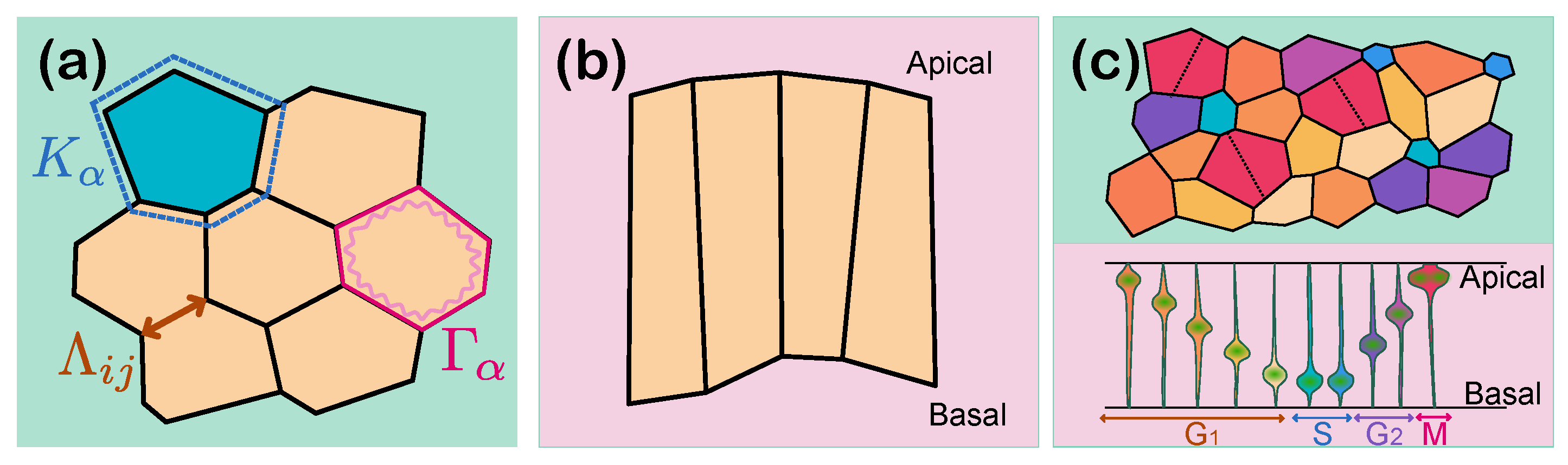
One of the most widely used formulations of the potential energy is based on surface and line tensions between cells described as 2D apical packing. In these models, the total energy E of the system is given by [4]:

$$E=\sum _{\alpha }{\displaystyle \frac{K_{\alpha }}{2}}{(A_{\alpha }-A^0)}^2+\sum _{\alpha }{\displaystyle \frac{{\Gamma }_{\alpha }}{2}}{L}_{\alpha }^2+\sum _{i,j}{\Lambda }_{ij}{l}_{ij},$$

(3)

where $\alpha$ is an index running over each cell in the tissue and the indices $i,j$ run over each pair of connected vertices (see Figure 1a). The first term in Equation (3) typically represents the surface elasticity of the cells, reflecting the cell’s resistance to deviations from a target area $A^0$ set by cytoplasmic or osmotic forces, with $K_{\alpha }$ as the elastic coefficient. Similarly, the second term introduces elastic energy depending on the cell perimeter $L_{\alpha }$, usually associated with actomyosin-mediated cortical contractility, where ${\Gamma }_{\alpha }$ is the contractility coefficient of the cell. Finally, the third term describes the interfacial tension or adhesion between cells, with ${\Lambda }_{ij}$ being a line tension coefficient specific to the interaction between these two cells. The magnitude and sign of ${\Lambda }_{ij}$ can change depending on the interaction at the cell–cell interface, introducing forces that either increase or decrease the length of shared cell boundaries.

This energy function can also represent tissues from an apicobasal perspective, depicting the planar cross-section of an epithelium, known as lateral vertex models [22,23]. Here, cells are represented by quadrilaterals spanning from the apical to basal sides of the cell (Figure 1b).

Following similar ideas, the vertex model has also been extended to three-dimensional vertex representations. In three dimensions, volume conservation becomes essential, introduced by an energetic term to maintain a preferred cell volume, as outlined in [6,24,25]. A generalized energy function for this class of models is given by

$$E=\sum _{\alpha }{K}_A{\left(A_{\alpha }-A_0\right)}^2+\sum _{\alpha }{K}_V{(V_{\alpha }-V_0)}^2,$$

(4)

where the first term quantifies the energetic cost associated with deviations of the cell surface area $A_{\alpha }$ from its preferred area $A_0$, reflecting the balance between surface tension and adhesion forces, where $K_A$ modulates the elastic response of cell-cell interfaces. The second term, where $V_{\alpha }$ is the volume of each cell, represents the cell’s resistance to maintain a characteristic volume $V_0$ with a volumetric modulus $K_V$, thereby enforcing volume conservation within the three-dimensional model.

Other complexities can also be incorporated in three dimensions, such as heterotypic interfacial tension, which accounts for both the tension and interfacial area between different cell types [24] or an additional surface tension to represent cell faces that interact at the boundary with the surrounding medium [25].

Modern variations of vertex models incorporate modifications of the energy function (Equation (3)) to capture additional biophysical properties required to describe particular tissue types. For instance, in tissues such as the neural tube pseudostratified epithelium, cells undergo interkinetic nuclear migration (IKNM), where the nucleus migrates along the apical–basal axis of the cell in synchrony with the cell cycle. As a result of this, cells close to the mitotic phase present a larger apical surface than cells closer to the S phase. Guerrero et al. [26] proposed a time-dependent target area term $A_0\left(t\right)$ that captures these dynamics, where $A_0\left(t\right)$ depends on the cell cycle phase (Figure 1c). Thus, instead of defaulting to a more complex 3D description of the tissue, traditional 2D vertex models can still be employed, in this case introducing the dynamic area expression extracted from experimental observations

$$A_0\left(t\right)={\displaystyle \frac{1}{2}}\left((t-t_0)g_{\alpha }+1\right)\left(1+{\left(r_{\alpha }(t-t_0)\right)}^2\right).$$

(5)

Here, $t_0$ is the time at which the cell was born, $g_{\alpha }$ is the growth rate of the cell, and $r_{\alpha }(t-t_0)$ is an autonomous function describing the apicobasal position of the nucleus during the different phases of the cell cycle. This formulation accounts for the variation in the apical area as the nucleus migrates between the apical and basal surfaces during IKNM.

Adhesion dynamics also play a critical role in vertex models, particularly during processes like cell neighbour exchange and tissue remodelling. The Apposed-Cortex Adhesion Model (ACAM), developed by Nestor-Bergmann et al. [27], incorporates adhesion turnover to describe how cells slip past one another during neighbour exchanges. The energy associated with adhesion can be modelled as follows:

$$E_{\mathrm{adh}}=\sum _{\mathrm{junctions}}\left({\displaystyle \frac{k_{\mathrm{adh}}}{2}}{(d-d_0)}^2\right),$$

(6)

where $k_{\mathrm{adh}}$ represents the adhesion stiffness, d is the distance between opposed cortices, and $d_0$ is the equilibrium adhesion distance. Here, each vertex is defined as a geometric point where three or more cells connect via adhesions, rather than a simple material point. Traditional models often represent each cell junction individually, whereas ACAM treats the apical cortex as the primary mechanical driver of cell behaviour, described as a continuous, viscoelastic loop. ACAM also accounts for forces from adhesion complexes and shows that resistance to slippage between cortices regulates cell rearrangement and complex tissue structures during morphogenesis. This approach reflects the cortex’s physical properties more accurately, enabling a more nuanced response to mechanical forces across the cell network. Adhesion turnover affects the rate of cell junction deformation, as well as the formation of rosettes and other complex cell arrangements during morphogenesis [27].

Overall, while traditional models, like those by Farhadifar et al. [4], rely on static assumptions for the energetic formulation, newer models, such as those by Guerrero et al. [26] and Nestor-Bergmann et al. [27], explore how dynamically changing cell mechanical parameters may fundamentally alter tissue morphology and behaviour. Recent work has also shown that these biophysical dynamic mechanisms, introduce new time scales that need to be calibrated properly against the friction coefficient $\mu$ in Equation (3). Traditionally, $\mu$ has occupied a secondary role; nevertheless, recent work [28] shows that the choice of friction impacts tissue growth rates, cell morphology, and topological transitions in vertex models where the timescale of progression of cell cycle interacts with the relaxation timescale of the potential energy.

Moreover, additional relaxation timescales may arise if other degrees of freedom are considered beyond the vertices. This occurs, for instance, when the apical surface described is part of a spatially expandable or curved tissue with geometrical degrees of freedom that affect the energy terms. For instance, in the neural tube, the apical structure can be considered as a cylindrical curved sheet that grows radially as neural progenitors proliferate, resulting in an equation for the evolution of the tube radius R,

$${\mu }_R{\displaystyle \frac{\mathrm{d}R}{dt}}={\displaystyle \frac{\partial E}{\partial R}}=-{\displaystyle \frac{1}{R}}\sum _i{r}_i{\displaystyle \frac{\partial E}{r_i}},$$

(7)

where ${\mu }_R$ is the drag coefficient for the dynamics of the radius of the tube and is different from $\mu$ and needs to be calibrated against the rest of the dynamical scales of the system (see [26]). The third term in Equation (7) simply provides an alternative mathematical expression of the second term, using vertex positions as the variables showing how these new degrees of freedom seamlessly integrate within the vertex model framework. This principle was recently applied to the growth of the zebrafish heart [29], exploring how changes in cell mechanical state can drive tissue-wide stretch.

Another example that incorporates accurate biological considerations of tissue timescales can be found in a study by Erdemci-Tandogan and Manning [30]. This study further explored the role of cellular rearrangement time delays on the rheology of vertex models, integrating T1 delay times into their simulations to mimic molecular processes during T1 transitions. This modification allows for a more accurate representation of tissue mechanics, capturing the delay in cellular rearrangements due to molecular processes and its effect on tissue elasticity and morphology.

Extensions to the energy function can include additional energy terms related to other biophysical processes such as cell polarity. For instance, in [14], cells establish a directional distribution of polarity proteins across the tissue plane. To represent protein densities in the model, values can be assigned to the edges of the cells, allowing tissue dynamics to influence the reorientation of planar cell polarity. Alternatively, in [31], the authors integrated directional stress components aligned with cellular polarity fields. It also enables the simulation of tissues under non-uniform stress conditions, which are common during various developmental processes. These updated vertex models can simulate more realistic tissue behaviours during morphogenesis, such as directional elongation and differential growth by modelling how cells generate and respond to mechanical stresses anisotropically. This is a significant step toward linking genetic regulation and mechanical properties in developing tissues.

In all the energetic descriptions discussed in this section, the tissue dynamics result from an energy minimization framework, where energy is constantly dissipated as a result of the relaxation along the degrees of freedom of the model, which do not coincide exactly with the biophysical degrees of freedom of the system, e.g., vertex positions vs. membrane movement. While this simplification facilitates computational efficiency and model tractability, it will need additional revision including more accurate energetic descriptions of elastic storage and dissipation of energy. For instance, neglecting additional energy dissipation may lead to underestimation of the timescales required for cellular rearrangements or biased predictions of force distributions during processes like wound healing or cancer invasion. These enhancements aim to provide a more realistic representation of the non-equilibrium dynamics governing cellular interactions, improving the interpretative power of simulation results in scenarios where dissipation significantly impacts tissue behaviour.

3. 2D or Not 2D

Vertex models have traditionally been developed in two dimensions. In these two-dimensional vertex models, cells are typically assumed to exist within a single monolayer, where their movement is governed by interactions confined to the apical 2D plane. In this approximation, external forces out of the 2D plane, such as those from the extracellular matrix or the environment, can be usually projected into the cell vertices. Additionally, any changes in the third dimension, like apicobasal fluctuations, can be mapped onto the 2D plane. Since the foundational work of Nagai and Honda [12] in 2001, two-dimensional vertex models have been extensively applied to study various morphogenetic and biological processes. These include mechanical effects in epithelial tissues, such as contractile forces generated by the actomyosin ring [4], jamming transitions [19], wound healing [17], the representation of planar cell polarity pathways [14] or the modelisation of growing epithelia [13,32], among many others. Some examples have already been introduced in Section 2 (see Equations (5) and (7)), introducing pseudo-3D descriptions that keep the numeric simplicity of traditional vertex models. Similarly, the same formulation can be easily used to study other geometrical projections of the tissue. For instance, a variant of two-dimensional vertex models consists in representing the planar cross-section of an epithelium, known as lateral vertex models. In this approach, cells are represented by quadrilaterals that depict the apicobasal surface of the tissue (Figure 1b). Naturally modelling the mechanical bending properties of the tissue, this model has been utilised to study phenomena such as Drosophila mesoderm invagination [23] and locally tubular epithelial folding [22].

Also, to model epithelial folding, another variant of the vertex model uses a 2D manifold of non-flat polygons with curvature to represent the epithelial surfaces. This approach has been applied to study phenomena such as the buckling of flat epithelia under compression [33] and the morphogenesis of respiratory appendages on Drosophila eggshells [34].

Nevertheless, there are scenarios in which 2D descriptions are insufficient for accurately modelling complex biological systems such as organoid development, tumour growth, or 3D cellular aggregates, where a three-dimensional approach is essential [18]. Extending vertex models to three dimensions presents several challenges. To describe tissue behaviour accurately, it is necessary to account for the mechanical polarisation of cells along the apicobasal axis, which requires defining distinct interactions at the apical, basal, and lateral surfaces, as well as the influence of the extracellular matrix. Also, computational complexity increases when simulating key processes that shape tissues, such as cell growth, division, apicobasal intercalation, and extrusion or apoptosis.

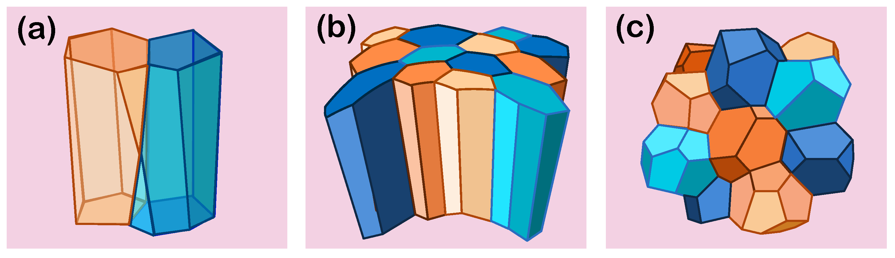
Honda et al. [6] introduced the first 3D vertex model to simulate cell aggregates, where cells are represented as space-filling polyhedra with vertices where four cells meet, connected by edges that form the polygonal faces of the cell boundaries (Figure 2). Like 2D models, the main objective is to study how cells deform and rearrange under external forces by minimising the total free energy. However, in the 3D model, the focus expands from conserving the area or perimeter of cells to conserving their volume, as noted in Equation (4). The strengths and limitations of the 3D vertex model compared to the 2D are highlighted in Table 1.

The distinction between apical and basal surfaces in the three-dimensional model allows for the consideration of cell polarisation by accounting for mechanical interactions at both surfaces and along the lateral interfaces and with the extracellular matrix. Polarisation plays a critical role in epithelial morphogenesis, leading to the formation of structures such as follicles, tubes, and branching networks. This distinction also helps define neighbour relationships: in traditional 2D models, two cells are considered connected basally if they are also connected apically. However, recent studies [35,36] have shown that cells can have different neighbours on the apical and basal surfaces, leading to the discovery of a new geometric shape—the scutoid, which accommodates these variations in cellular organisation (Figure 2a).

When modelling tissue morphogenesis, three-dimensional vertex models allow for the accurate capture of cell reorganisation in 3D space and the interactions with their neighbours and the extracellular matrix (ECM), as well as the mechanical properties of the tissue. For instance, viscosity has been demonstrated to play a crucial role in tissue formation and development. The morphology of epithelial cysts is highly sensitive to the viscosity of the surrounding extracellular matrix: low viscosity results in straight tube formation, intermediate viscosity induces buckling and branching, while high viscosity leads to thickened and undulated tubes [37]. In addition, different 3D descriptions result in different strain properties of the tissue, such as the Young’s modulus and Poisson ratio, required to recover specific buckling properties of epithelial monolayers [38]. Similarly, forces along tissue surfaces, such as apical contractility, contribute to maintaining homogeneous curvature in epithelial sheets despite mechanical disturbances from cell division [39] (Figure 2b). These fundamental aspects of morphogenesis can provide insights into tumourigenesis, as disruptions in these normal mechanical and biochemical processes can lead to abnormal cellular behaviours and tumour formation. For instance, the morphology of epithelial tumours in the pancreas is influenced by the interplay between these parameters and the existing tubular geometry, which results in distinct growth patterns shaped by duct size and underlying mechanical forces [40]. Also, a recent study has provided the first evidence that defective cell–cell linkages, abnormal interactions with the extracellular matrix, and a favourable three-dimensional tissue structure can drive cancer invasion [41,42].

Biological processes during morphogenesis are driven by the regulatory activities of proteins and other cellular components. In three-dimensional vertex models, the intercellular transport of molecules is represented through the integration of reaction-diffusion systems within the cellular framework. This approach allows for the coupling of pattern formation dynamics with the chemical states of individual cells, facilitating a deeper understanding of the biochemical and mechanical processes that lead to tissue deformation and epithelial growth, including the study of Turing patterns that emerge from these interactions [43,44].

Three-dimensional vertex models are particularly useful for studying how cells within an organoid interact, rearrange, and respond to mechanical forces. An organoid is a three-dimensional miniaturised, simplified version of an organ that is grown in vitro from stem cells. These organoids mimic the key structural and functional characteristics of their corresponding in vivo organs. They have emerged as an important tool in personalised medicine, drug discovery, and regenerative medicine, enabling insights into how organs develop, how diseases progress, and how therapies can be optimised [45].

Recent studies have advanced the understanding of organoid development through various approaches. For instance, in [46], researchers developed a mechanistic theory of epithelial shells that resemble small organoid morphologies derived from invaginated structures and in [47], three-dimensional cellular forces are mapped in mouse intestinal organoids grown on soft hydrogels, revealing a non-monotonic stress distribution that delineates mechanical and functional compartments within these structures. Moreover, the flexibility of a human colon epithelium monolayer is studied in [48] using a combination of vertex modelling and finite element methods (FEM) and very recently, topological defects such as cysts and intestinal organoids have been explored in spherical epithelia [38].

Additionally, in modelling non-epithelial confluent biological tissues, 3D vertex models effectively represent the behaviour of heterotypic interfaces between different cell types [24]. This approach aligns closely with experimental observations of cellular behaviour at tissue boundaries, such as those in the Xenopus gastrula.

In summary, transitioning from two-dimensional to three-dimensional vertex models marks a critical step forward in understanding tissue morphogenesis. Research progresses towards more precise and sophisticated three-dimensional vertex models, bringing us closer to fully capturing the intricate processes of tissue dynamics.

4. How Many Sides Does a Cell Have Anyway?

Traditional vertex models assume that the apical surfaces of cells can be described by polygonal packing in confluent tissues. However, this imposes a rigidity on cell shape and movement that does not align with the more fluid behaviour observed in some cell communities, where dynamic, non-linear cell boundaries are present. Inspired by active foam models, vertex descriptions overcoming these limitations have arisen relaxing two of the basic assumptions of traditional vertex models [49,50]: (1) each cell can be described by more vertices than its tricellular junctions [49], and (2) internal vertices can belong exclusively to a single cell. As a result, cells can be described as polygons with a high number of sides, increasing at the same time the resolution and the computational complexity of the system. These descriptions also allow for a more nuanced mechanical description of local cortical tensions and pressures at a cell intrinsic level which impacts the deformation and motility of these cells resulting from the stress relaxation in the tissue.

For instance, in [51], cell populations are described by a mixture of cells and extracellular spaces, all of them with an arbitrary number of vertices. Extracellular spaces are described as a cell type of their own, with specific physical properties. To allow for sufficient freedom in the evolution of cell shapes and spaces, cell perimeter constraints (typically based on cortical actomyosin ring dynamics, as in Equation (3)) are replaced with local tensions at each vertex, along with cellular and extracellular pressures. This removes the convex polygonal signature often required for traditional vertex models and allows for tissue fluidisation (Figure 3b).

An even more flexible approach is introduced in PolyHoop [10], where each individual cell is described by a customisable number of vertices. Hence, this model allows for the formulation of interaction potentials that account explicitly for cell–cell interaction, enabling the incorporation of complex cellular contact dynamics between adjacent cell boundaries that are not captured by traditional vertex models (Figure 3c). In addition, the increased resolution allows the introduction of bending energies that regulate cell deformation beyond the classical elastic dilations of area and perimeter.

The additional flexibility of these models also introduces more nuanced descriptions of topological transitions. In the case of [51], through the merging of extracellular vertices due to cell–cell contact. On the other hand, in PolyHoop, topological changes are related to changes in the number of polygons due to excision or merging events.

While these descriptions introduce a natural way of studying fluidity, confluence, or non-straightness of boundaries; these properties are not exclusive of highly sided descriptions, and can also be obtained by self-propelled Voronoi models [19], as it is discussed in the next section.

5. Out of the Vertex

An alternative way to formulate the mechanics of tissues is the self-propelled Voronoi model (SPV) [19], sometimes also called the active vertex model [52]. As opposed to traditional vertex models, cells are described by the location of their centres. Here, the geometry of a polygonal tissue is parameterised by the Voronoi tessellation of the (circum) centres of each of the cells. Dynamics progress with overdamped kinetics of the cell centres minimising an energy function, which is typically identical in nature to traditional vertex models (see Equation (3)). Additionally, cells can undergo migration or self-propulsion, where an active velocity with constant speed ($v_0$) is applied to each cell. Thus, for each cell centre $x_i$ of a cell i, its velocity is given by

$${\displaystyle \frac{\mathrm{d}{x}_i}{\mathrm{d}t}}=-\mu {\displaystyle \frac{\partial E}{\partial x_i}}+v_0{\widehat{n}}_i,$$

(8)

where ${\widehat{n}}_i$ describes the propulsion orientation of each cell and E is the corresponding energy function. This propulsion could in principle be purely Brownian, yet given cell migration is typically persistent in nature, some studies propose other functional forms. For instance, in [19], the random normal vector ${\widehat{n}}_i$ has an angle $\theta$ following the Langevin (SDE) equations:

$$\begin{array}{cc}\hfill {\displaystyle \frac{\mathrm{d}{\theta }_i}{\mathrm{d}t}}& ={\eta }_i,\left(t\right)\hfill \end{array}$$

(9)

$$\begin{array}{cc}\hfill \langle {\eta }_i\left(t\right),{\eta }_j\left(t^{\prime }\right)\rangle & =2D\delta (t-t^{\prime }){\delta }_{ij},\hfill \end{array}$$

(10)

introducing a persistence timescale on the motion, $1/D$.

In SPV, topological transitions are automatic, without requiring rules for T1 transitions. This is because the cell neighbourhoods are generated by Voronoi tessellation: if two cells become close enough, the neighbourhood will be established by the tessellation. For vertex models (either traditional or SPV), the prevalence of T1 transitions is determined by the mechanical description of the tissue, becoming energetically disfavoured easily in ‘solid’ parameter regimes, a common disadvantage of vertex models. Self-propulsion (see Equation (8)) allows cells to overcome small enough energy barriers, fluidizing the tissue with increasing propulsion speeds, or increasing persistence time-scales [19].

The self-propelled Voronoi model can thus be viewed as an active variant of the traditional vertex model, with half the number of degrees of freedom. This constrains cells to a specific geometric space. Assuming that cell geometries evolve in time through continuous force balance over medium time-scales—a proposal for which there is some empirical support [20] and is the founding principle of force inference [53]—the true geometric space that cells explore will have $3N_{cell}/2$ degrees of freedom, more restricted than the vertex model ($2N_{cell}$) and less restricted than the Voronoi model ($N_{cell}$). Future work matching this geometric constraint by extending the Voronoi model towards Dirichlet cell complexes [20] could allow researchers to marry the computational and physical benefits of the vertex model with the more geometric realism of the traditional vertex model.

6. Mechanochemical Feedback in Heterogeneous Populations

Many of the complexities of multicellular dynamics—both in development and disease—arise from interactions between distinct cell types. These mechanical or chemical interactions can occur over different length scales. Indeed, the interplay between physical interactions, cell and tissue geometry, intercellular signalling, and cell fate can facilitate emergent properties of multicellular collectives that cannot be reduced to its comprising components [54]. Consequently, integrative modelling frameworks that can combine these multifarious contributions to the emergence of order in development, or its modification and erosion in disease, are starting to act as important test-beds to understand the necessary components for sets of multicellular behaviours and establish experimental predictions to distinguish between alternative mechanochemical mechanisms.

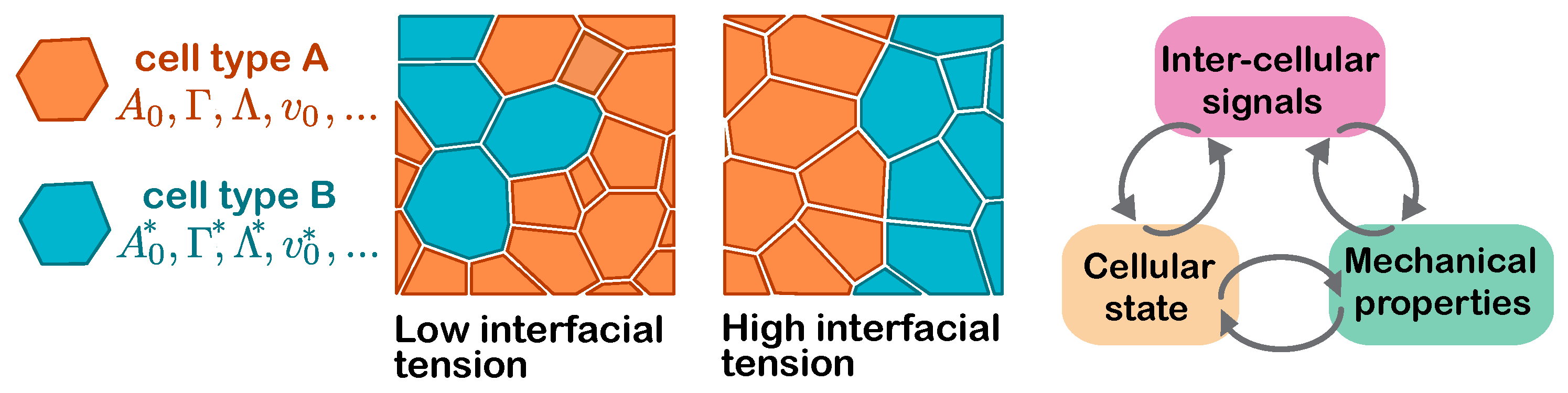
Given their cell-centred nature, vertex models and their derivatives are ideal computational frameworks to simulate emergent multicellular dynamics due to mechanochemical feedback. One can define distinct mechanical parameters for each individual cell, or indeed sets of cells falling into one or more cell type. For example, multi-state vertex models, simulating differential interfacial tension between different cell types, has been shown to mediate lineage segregation boundary integrity [55], cell elimination and cyst formation in Drosophila imaginal discs [56] (Figure 4). These concepts were further extended to discern the distinct morphological modes of tumourigenesis in different carcinomas, where mutant and neighbouring wild-type cells were modelled to have different mechanical properties, allowing the researchers to establish a morphospace of multi-layered tumours and map these onto driver mutations [57]. Likewise, a 3D vertex model of zebrafish heart morphogenesis has been used to explain how a gradual change in the frequency of cells that relax their junctional tension can result in a sudden, dramatic increase in heart size [29]. Beyond ‘steady-state’ cell-type specific mechanical properties, the vertex model, being a dynamic model, has the potential to unpack how cell-state-dependent mechanical fluctuations can modulate the emergence of order. Using 2D and 3D vertex modelling coupled to dynamic measurements, a recent study has proposed that the segregation of the extraembryonic primitive endoderm from the embryonic epiblast in the mouse blastocyst occurs by enhanced cell surface fluctuations in the former tissue [58].

Mechanosensation allows tissues to close the feedback loop between mechanical properties and cellular state. Cell-centred modelling frameworks are natural simulation frameworks that analyse these interactions. Including a cell decision layer on top of the traditional vertex model that modulates cell-cycle status or the probability of apoptosis as a function of a cell’s adhesion status, shape and local density, can result in emergent, self-organising patterns of proliferation and tissue growth control [59]. Similarly, the coupling between tissue mechanics and cell shape has been used to analyse how cell geometry and stress influence the orientation of planar cell divisions [60].

Coupling can also be achieved at the tissue scale by the modulation of tissue rheological properties. For example, the self-propelled Voronoi (SPV) model was recently used to analyse the interplay between ERK-signalling, tissue rheology, cell density, and cell migration, identifying how the relative contributions of each regulate a dynamical transition from static ‘glassy’ behaviour to spatiotemporal oscillations [61]. Global transitions in tissue rheology can also shape physiological response to injury: a recent work studying coupling measurements of clone fragmentation with in vivo lineage tracing with 2D the (SPV) model established that changes in local cell density upon cell ablation promote the transition from a ‘solid’ to a ‘fluid’ tissue state, which in turn activates stem-cell renewal to restore the tissue to homeostasis [62].

To generalise cell-centred modelling frameworks beyond purely mechanically mediated feedbacks, modelling efforts must connect cell shape and state with intercellular chemical signalling. Signalling may be contact dependent, as in Notch signalling, where vertex models have proved useful to understand the interplay between contact area, signal transduction and resultant patterning [63]. Signalling may alternatively be longer range via the establishment of morphogen gradients [44]. However, connecting the self-organisation of tissue morphology with its patterning remains challenging and incomplete in general, and yet is the key to understanding the elaboration of order during embryonic development, both natural and, through the use of organoids and embryos (stem-cell based embryo models), synthetic. Future work must build on the above successes to establish integrative computational frameworks to model cell state, mechanics and signalling in an integrative manner that is efficient enough to characterise its dynamical modes exhaustively with morphospaces and, importantly, constrain it to data to help devise and test mechanistic hypotheses.

7. Inference Makes the Difference

Inference of biologically relevant simulation parameters from measurements is a key quantitative application of vertex models and has led to considerable biological insight [26]. Nevertheless, these efforts are often hindered by the need to associate equivalent parameters in the model and experimental data, the considerable parametric degeneracy in simulation outputs, and non-identifiability in some specifications of vertex models. In this section, we describe recent progress in these areas, including how more accurate descriptions of physical effects, such as those described in previous sections, lead to more robust inference, and how advances in Bayesian inference provide a natural framework for extracting quantitative insights.

The task, as in any inference framework, is to provide information of the set of parameters $\theta$ compatible given a specific tissue observation—the data $\mathcal{D}$. For instance, for the energy function (Equation (3)) we would typically have $\theta =\{A^0,K,\Gamma ,\Lambda \}$, and the data $\mathcal{D}$ as an image of a tissue. In Bayesian inference, our knowledge of the true values of specific sets of parameters is formally quantified as a posterior credibility distribution $p\left(\theta \right)$ [64]. These are also traditionally referred to as probability distributions. Nevertheless, the parameters that need to be inferred are deterministic: the distributions only reflect quantitatively our uncertainty on this deterministic value. Therefore, the distributions are not directly related to any randomness in the values of the parameters. For this reason, we avoid the term probability in favour of the term credibility, as advocated by Kruschke [64]. These distributions give more weight to parameter regions that are more likely (have more evidence) to match a specific observation. The distributions $p\left(\theta \right)$ follow the same rules as classical probability distributions, unlocking the toolkit from probability theory. In particular, we can update our distributions given a dataset $\mathcal{D}$ using Bayes’ theorem,

$$p\left(\theta \right|\mathcal{D})=\mathcal{N}p(\mathcal{D}\left|\theta \right)p\left(\theta \right),$$

(11)

where $p\left(\theta \right)$ represents the prior distribution of the simulation parameters before the observation of the data, and $p\left(\theta \right|\mathcal{D})$ is the posterior distribution containing the updated knowledge provided by the data $\mathcal{D}$. They are related by the normalization constant $\mathcal{N}$ and the likelihood $p\left(\mathcal{D}\right|\theta )$. The normalization constant $\mathcal{N}=p\left(\mathcal{D}\right)=\int p\left(\mathcal{D}\right|\theta )d\theta$ is in general hard to calculate but is in practice unnecessary as we usually rely on relative credibilities for hypothesis testing. On the other hand, the likelihood $p\left(\mathcal{D}\right|\theta )$ states how likely would be to observe the data for different hypothetical values of $\theta$. This likelihood has no closed-form expression, so evaluating Equation (11) as it stands is intractable. However, we can use vertex model simulations to generate instances of the data from the simulation for given sampled parameter sets from the prior distribution ${\theta }^{\ast }\sim p\left(\theta \right)$, keeping parameter sets $\theta$ that are compatible with the observed data, allowing us to use Equation (11) to update our credibility distributions.

In practice, the inference process also requires us to compare observed and generated datasets which are inherently stochastic, i.e., the same parameter will result in different specific positions of the cells. Therefore, we need to define some metric $d_{\theta }$ to compare quantitatively the resulting datasets. This is usually performed by computing summary statistics, which capture the key features of both real and simulated data. We can then calculate the distance between the summary statistics of real and simulated data, providing a measure of how close the simulated samples are to the true data (and therefore also the posterior distribution of the simulation parameters). This is the idea that underlies approximate Bayesian computation (ABC), where posterior samples are approximated by selecting parameters that minimize the distance metric (Figure 5). Here, there are still several open questions relating to which summary statistics sufficiently discriminate good and poor matches to the real data [65], the distance metrics to use [66], and the convergence properties of the ABC algorithm itself. These are in addition to problems common to all Bayesian inference tasks, such as the selection of reasonable prior distributions. In simulation-based inference tasks, this is complicated by the unknown relationship between the simulation parameters and the effective likelihood, so selection based on intuition alone is difficult [67].

The ABC method has proven particularly useful when determining underlying biological parameters in vitro by comparison to experimental data [68,69,70]. Furthermore, the approaches presented here can also actively inform experimental design, optimising the informational content of an experiment relative to both the biological model in question and the inference method [71].

In addition to the simple rejection ABC formulation described above, there are a number of modifications that can be made to improve the efficiency of the sampling step. It is often difficult, particularly initially, to obtain samples from $p\left(\mathcal{D}\right|\theta )$ that are close to the target dataset $\mathcal{D}$. In ABC-MCMC [72], proposal samples are generated with an additional Markov chain Monte Carlo step along the prior distribution, $p\left(\theta \right)$, in a form analogous to the classic Metropolis-Hastings algorithm. Here, samples are first drawn from a proposal distribution centred on the previous value and are then accepted according to the distance metric $d_{\theta }$, as in rejection ABC. Sequential Monte Carlo (ABC-SMC) [73], an alternative sampling strategy, utilises a variable value of the distance $d_{\theta }$ threshold, $\epsilon$. At the start of the sampling, $\epsilon$ is large and is reduced sequentially. Each evaluation of the distance for a specific dataset requires a full vertex model simulation. Nevertheless, as there is no dependence between the evaluated parameter sets, $\theta$, sampling and evaluation can proceed in parallel, making the inference process computationally efficient.

Whilst Bayesian inference provides an automatic way to update quantitatively our beliefs in specific parameter sets, it can be computationally demanding. Recent advances in the field attempt to accelerate this inference process by developing neural networks to sequentially estimate approximations to the full posterior density, such as sequential neural posterior estimation [74], or to the likelihood, such as sequential neural likelihood estimation [75]. These can be viewed as the logical endpoint of the kind of improvements exhibited by adding sequential updates to standard rejection ABC. Instead of approximating the posterior distribution by an n-ball in distance space, a neural network is employed to use the samples to sequentially refine a more complex representation of the posterior density. An additional advantage of these methods is that they are constructed to learn a posterior independent of the specific dataset they are initially trained on. This amortised strategy means that posterior probabilities of related experiments can be inferred without full re-optimisation of the model, and moreover, can be used to improve the estimate of the posterior.

Common summary statistics include ‘primary’ statistics specific to individual cells, such as cell elongation and cell area ratios, and ‘secondary’ statistics that are bulk properties of the simulated tissue, such as the number of neighbours and their area. For the relative area and perimeter terms, regardless of which individual statistic is chosen, it is difficult to determine uniquely the value of either, as the posterior distributions are highly correlated [67]. However, combinations of statistics constrain the parameter space better, and estimates improve with increasing dataset size, indicating that this is not an inherent degeneracy of the model. Nevertheless, the difficulty of inference of energetic parameters in classical energetic descriptions (Equation (3)) implies that reformulating the model may be an avenue to more efficient inference with ABC.

The exact specification of the model and inference procedure can also significantly influence results [76]. In particular, misspecification of the model for a particular regime can result in spurious correlations, leading to incorrect conclusions regarding parameter values and their relative importance to the system. For example, as noted in [28], the addition of an explicit friction parameter can affect static and dynamical properties of the model, features that otherwise would be implicitly and incorrectly associated with other terms. On the other hand, a model theoretically and empirically well motivated, such as those described in the previous sections, can be impossible to fully determine in practice. In [67], the authors performed a ‘closure’ test, where data generated from a model is fitted using the same model in order to probe practical issues of parameter identifiability. With a range of standard summary statistics, and with a small dataset, it is not possible to uniquely recover parameters from a model that the data was generated with. However, with the aforementioned ‘secondary‘ statistics and larger datasets, parameters are rendered identifiable. This underscores the importance of performing tests for parameter recoverability and indicates that more work still remains to optimally specify vertex models and their associated summary statistics. Similarly, constructing accurate likelihood functions that account for artefacts and noise in specific experimental datasets is paramount for achieving unbiased mechanistic inference of the biophysical mechanisms governing tissue dynamics.

8. Discussion

The continued evolution of vertex models reflects both the growing complexity of biological questions and the expanding computational capabilities available to researchers. While early models succeeded in capturing key mechanical aspects of tissue dynamics, modern approaches are now capable of addressing more intricate questions. Some of the main modelling strategies identified are summarized in Table 1.

One of the primary challenges is the balance between model complexity and computational efficiency. As our understanding of tissue dynamics improves, the desire to include more detailed mechanistic insights, such as cell cycle dynamics, intercellular signalling, and anisotropic stresses, increases. While such details are critical for accurately simulating real biological processes, they come at the cost of computational complexity, which can limit the scalability of the models. This is especially true for 3D vertex models, where accounting for the intricate interactions at apical, basal, and lateral surfaces significantly increases the number of parameters and the computational resources required. Moreover, the introduction of 3D models presents new geometric and physical challenges. The discovery of scutoids as a geometric solution for packing in 3D epithelia illustrates the limitations of classical 2D descriptions in representing realistic tissue behaviours [35].

To address some of the limitations of traditional vertex models without the requirement of a taxing 3D description, new 2D frameworks have been developed in the last years, such as those allowing cells to have more vertices than just those corresponding to the tissue boundary and its junctions [10,51] or cell-centred models such as the SPV.

Another major area of focus in the last years has been increasing the mechanochemical feedback, which plays a pivotal role in tissue morphogenesis. Understanding how mechanical forces and biochemical signals interact to influence cell fate and behaviour is critical for simulating complex developmental processes.

Together with the development of a more complex modelling framework, recent works have focused on the inference process, addressing the merging of models and data and improving our ability to explore parameter spaces. These studies revealed that many models still suffer from non-identifiability and parameter degeneracy, limiting their predictive power. Ultimately, these results highlight the path forward in the future of vertex models that need to evolve together with their inference capabilities.

In conclusion, while vertex models have made tremendous strides in recent years, there are still substantial challenges to overcome. Future work should focus on improving the balance between model detail and computational feasibility, refining parameter inference techniques, and developing integrated frameworks that combine mechanical, biochemical, and signalling dynamics.

In addition, we identified a significant lack of benchmarking studies comparing various vertex model approaches. Conducting such studies could provide valuable insights into the efficiency and limitations of different implementations, guiding future advancements in the field.

As these challenges are addressed, vertex models will continue to be indispensable tools for understanding the complexities of tissue morphogenesis and cellular dynamics.

Table 1. Different vertex model (VM) implementation strategies.

Model	Strengths	Limitations	Refs.
Traditional 2D	- Computational simplicity/speed - Extensively studied with robust, efficient implementations across diverse contexts	- Unable to represent complex cell morphologies - Unable to model 3D processes (e.g., organoids)	[4,9,12,14,17,19]
Pseudo-3D VM	- Describes 3D effects without requiring additional computational complexity - Can incorporate extra degrees of freedom such as nuclear apicobasal nuclear position	- Careful parameter tuning for accuracy - Unable to incorporate complex 3D dynamics	[26,30]
3D VM	- Realistic representation of 3D morphogenesis - Captures apicobasal interactions and interactions with the extracellular matrix - Not limited to epithelial monolayers	- High computational complexity - Requires additional parametrisation of tension, adhesion and volume conservation. - Difficult calibration of parameters with experimental data	[6,24,25,37,39,40,44]
High resolution VM	- Improved resolution of local cell–cell interaction dynamics. - Captures local tensions and pressures in greater detail - Precise representation of cell deformations and motility	- Higher computational complexity - Lack of benchmarking	[10,51]
SPV	- Simpler handling of topological transitions - Fewer degrees of freedom than traditional models	- Inaccurate to represent complex cell geometries. - Loss of local mechanical descriptions due to geometric constraints.	[19,20,52,53]

Table 1. Different vertex model (VM) implementation strategies.

Model	Strengths	Limitations	Refs.
Traditional 2D	- Computational simplicity/speed - Extensively studied with robust, efficient implementations across diverse contexts	- Unable to represent complex cell morphologies - Unable to model 3D processes (e.g., organoids)	[4,9,12,14,17,19]
Pseudo-3D VM	- Describes 3D effects without requiring additional computational complexity - Can incorporate extra degrees of freedom such as nuclear apicobasal nuclear position	- Careful parameter tuning for accuracy - Unable to incorporate complex 3D dynamics	[26,30]
3D VM	- Realistic representation of 3D morphogenesis - Captures apicobasal interactions and interactions with the extracellular matrix - Not limited to epithelial monolayers	- High computational complexity - Requires additional parametrisation of tension, adhesion and volume conservation. - Difficult calibration of parameters with experimental data	[6,24,25,37,39,40,44]
High resolution VM	- Improved resolution of local cell–cell interaction dynamics. - Captures local tensions and pressures in greater detail - Precise representation of cell deformations and motility	- Higher computational complexity - Lack of benchmarking	[10,51]
SPV	- Simpler handling of topological transitions - Fewer degrees of freedom than traditional models	- Inaccurate to represent complex cell geometries. - Loss of local mechanical descriptions due to geometric constraints.	[19,20,52,53]