Emergence of Diverse Epidermal Patterns via the Integration of the Turing Pattern Model with the Majority Voting Model

Abstract

Animal skin patterns are increasingly explained using the Turing pattern model proposed by Alan Turing. The Turing model, a self-organizing model, can produce spotted or striped patterns. However, several animal patterns exist that do not correspond to these patterns. For example, the body patterns of the ornamental carp Nishiki goi produced in Japan vary randomly among individuals. Therefore, predicting the pattern of offspring is difficult based on the parent fish. Such a randomly formed pattern could be explained using a majority voting model. This model is a type of cellular automaton model that counts the surrounding states and transitions to high-number states. Nevertheless, the utility of these two models in explaining fish patterns remains unclear. Interestingly, the patterns generated by these two models can be detected among very closely related species. It is difficult to think that completely different epidermal formation mechanisms are used among species of the same family. Therefore, there may be a basic model that can produce both patterns. Herein, the Turing pattern and majority voting method are represented using cellular automata, and the possibility of integrating these two methods is examined. This integrated model is equivalent to both models when the parameters are adjusted. Although this integrated model is extremely simple, it can produce more varied patterns than either one of the individual models. However, further research is warranted to determine whether this model is consistent with the mechanisms involved in the formation of animal fish patterns from a biological perspective.

1. Introduction

The Turing model is a type of reaction–diffusion (RD) model that was introduced by Turing in 1952 [1] and describes the patterns that arise due to Turing instability. Turing instability arises due to the interplay between active and inhibitory factors. Two types of diffusion coefficient substances (morphogens) are assumed as these factors in the model. In the 1980s, Meinhardt [2] demonstrated that the Turing model can create various patterns via computer simulation. However, due to the lack of concrete experimental evidence, for a long period, it was not recognized as a model that could explain pattern formations in living organisms. Instead, Wolpert’s “morphogen gradient model” [3,4] for the morphogenesis of organisms was considered to be the dominant model. However, even Wolpert’s model could not explain the robustness of the actual morphogenesis of organisms because of the dependence on the initial values and the vulnerability to disturbances. Thus, a definitive model for such morphogenesis remains unavailable.

Pattern formation was first identified in an actual animal using the Turing model in the 1990s by Kondo and Asai [5] in sea anemones (Pomacanthus imperator). Regarding hybrids, Miyazawa et al. [6] compared the patterns of pure and hybrid species of salmonid fish and reported that each pattern could be explained by solving the Turing model equation and that the hybrid pattern could be reproduced by considering intermediate values of the parameters that reproduced the patterns of pure species. Milinkovitch et al. [7] discussed the efficacy of the RD systems, which can actually capture most of the functionally relevant behaviors of skin color patterning without needing to parameterize the unmanageable profusion of variables at the nanoscopic and microscopic scales.

Conversely, the proteins or chemicals that are responsible for morphogenesis have not been identified, although some candidate substances (e.g., signaling factors such as TGF-β, Wnt, and Dkk [8,9], as well as Hox gene products [10]) have been reported. Dilão et al. [11,12] showed that mRNA diffusion is the primary morphogenetic mechanism that consistently explains the establishment of bicoid protein gradients in the embryo of Drosophila. Recent experimental studies have shown that the function of morphogens is not limited to the distribution of chemical concentrations, and they are involved in cell–cell interactions [13,14,15,16]. These experimental studies revealed that the diffusion of chemicals is not the only factor that forms Turing patterns; instead, these patterns include the autonomous movement of pigment cells [17] or cell–cell signaling via cell protrusions [18,19]. This is the specific case of the zebrafish pattern. Such cases should be considered as patterns that emerge due to Turing instabilities, which are satisfied under conditions similar to certain diffusion coefficients. Although the biochemical mechanisms of pattern formation remain unclear, the experimental manipulation of patterns has elucidated that the formation of certain body patterns is consistent with the models of the RD equation, such as the Turing model; this is commonly accepted among biologists [20]. Furthermore, pattern formation is possible even in the absence of chemical diffusion if the conditions required for the interaction between local activation and long inhibition, with nonlinear effects, are satisfied [21,22].

Computer models have also been developed that more faithfully reproduce the realistic pattern formation processes that have been elucidated based on these experiments. For example, several simulations have been developed using agent-based models to reproduce zebrafish pigment pattern formation [22,23,24,25]. Vasilopoulos and Painter [26] also constructed a model with interacting cell protrusions and observed that, even if the protrusions are not anisotropic, the adjustment of their length and density can produce patterns that are similar to the RD model. In addition, Marcon et al. [27] investigated whether a stable stationary wave pattern can be generated in a three-factor RD system. Moreira and Deutsch [28] presented a model depicting pigment-cell pattern formation in zebrafish based on the local interaction cellular automata (CA) model, demonstrating the importance of differential intercellular adhesion and the mechanisms of stem cell regulation. Konow et al. [29] proposed a lattice-based “survival model” based on recent findings on the nature of long-range chromatophore interactions and found that the model produces stationary patterns using diffuse stripes and undergoes Turing instability. Owen et al. [30] constructed an individual-based mathematical lattice model of the zebrafish skin pattern that incorporated all important cell types and known interactions. They reported that the model strongly supports the validity of these experimental interpretations, a fact which compels further detailed investigation into their molecular bases. In turn, Ishida et al. [31] developed a pufferfish skin pattern model using a CA model. This CA model was based on Turing patterns through the exchange of binary values between neighboring cells. Despite the simplicity of the model, which uses five parameters (three parameters related to basic color patterns and two parameters for the creation of a large black spot), it was able to produce the skin patterns of Takifugu. Zakany et al. [32] reported that the dynamics of the color flipping of Timon lepidus can be modeled using a stochastic cellular automaton.

Examples of discrete models outside these studies include Graner and Glazer [33], who simulated the sorting of a mixture of two biological cell types using a modified version of the large-Q Potts model with differential adhesivity. Dilão et al. [34] devised a reaction–diffusion model that considers two diffusive morphogens and three nondiffusible pigment precursors to simulate the general structural organization, phenotypic plasticity, and seasonal variation of eyespots (a concentric motif on butterfly wings). Several studies [31,32,33,34] have shown that various animal skin patterns are strongly dependent on the region and dimension of the skin structure of the target animal.

As a more generalized model, Kondo proposed the Kernel–Turing (KT) model [35], which uses distance and response profiles (i.e., kernels) to indicate activity and inhibition and performs convolution integrals of these parameters to generate Turing patterns. Simulations of the KT model with kernels of various shapes have shown that, in addition to being able to generate all standard patterns, i.e., stable 2D patterns (spots, stripes, and networks), it can also generate complex patterns that are difficult to generate using conventional Turing models.

Thus, models of the formation of animal epidermal patterns have long been studied based on the Turing model. Nevertheless, can we assume that all epidermal patterns in animals can be explained by the Turing model (or similar, related models)? Previous studies have classified the body patterns of various fish [36] and it has been reported that the more typical Turing pattern is limited to a few of these species. The KT model [35] can also form derivative patterns other than the typical Turing pattern.

However, even among fish, some individuals clearly do not exhibit Turing patterns, differing significantly from the patterns that can be generated using these models. For example, the body pattern of the ornamental carp Nishiki goi (Cyprinus carpio) produced in Japan varies randomly from individual to individual. Nishiki goi is the generic name of a variety of carp that has been improved for use as an ornamental fish. Various patterns have been created by crossbreeding these fish, including two-color red and white patterns and three-color white, red, and black patterns, as shown in Figure 1A. Patterns vary randomly from individual to individual and it is difficult to predict the offspring pattern based on that of the parent fish. For example, Figure 1B presents an example of a two-color Nishiki goi (red and white) in which the arrangement of the red pattern is different in every individual. Figure 1C presents an example of a three-color Nishiki goi (red, white, and black) in which the pattern mixture varies among individuals. Although genetic studies of carp body coloration have been published, such as [37], no studies on the reproduction models of these patterns are available.

The example of Nishiki goi patterns is similar to that of the black and white pattern of Holstein cows and the pattern of calico cats (tortoiseshell and white cats). The body patterns of these animals are genetically determined by the presence of two or three colors, whereas the shape of the pattern is randomly determined. In 2002, Qiu J. et al. [38] reported the birth of a somatic cell nuclear transplant clone of a cat. The nucleus was donated by a calico cat, the surrogate mother that gave birth to the cloned animal was a tiger cat, and the cloned cat was a calico cat. However, the patterns of the calico cat that donated the nucleus and that of the cloned cat exhibited different formations [38]. Although it is clear that genetic factors determine the number of colors in the pattern, the mechanism via which the pattern is formed on the body surface remains under study. The modeling analysis in the study did not consider a three-color model but only a two-color pattern. Although a three-color model can possibly be similarly explained by extending the same model, this is a subject for future investigation.

The majority voting rule model proposed by Vichniac is an explanatory model in which these animal patterns are formed randomly [39]. The model is a CA model (the state can be 0 or 1) that uses the sum rule of the Moore neighborhood (eight adjacent cells) via the majority vote, where the focused cell is 1 if the sum of the surrounding cells is 5 or more and 0 if the sum is less than 5. The time evolution of this model from a random initial state strongly depends on the ratio or distribution of the 1 and 0 statuses in the initial state. It has been reported that, given proper initial placement, it is possible to form animal patterns using this model.

The epidermal pattern of Nishiki goi may also be explained by this majority rule model. The pattern differences observed among individuals are attributed to slight differences in the conditions present during the growth process, and they can be thought of as corresponding to the sensitivity of the majority voting model to the initial values. From this, it can be inferred that the epidermal pattern of some fish can be explained by either the Turing pattern model or the majority voting model. To what extent can these two different models reproduce fish patterns?

Patterns from both of these models can also be found among extremely closely related species. For example, the Nishiki goi is a member of the carp family; however, the zebrafish, which is also a member of the carp family, has a Turing pattern; this pattern has been used to investigate many morphological models. Nevertheless, whether all fish patterns can be explained by these two different models remains unclear. However, interestingly, patterns arising from these two models can be detected among very closely related species. It is difficult to believe that completely different epidermal formation mechanisms are employed among species of the same family. Therefore, there may be a more basic model that can produce patterns via both models.

In this study, the Turing model and majority voting model are represented by CA, leading to the proposal of a new model that integrates these two models. After adjusting the parameters, this integrated model becomes equivalent to both previously mentioned models. Parameters that are intermediate between these two models can also be established. This integrated model produces a greater variety of patterns than either one of the two models. Although the model is extremely simple, it can produce a variety of patterns. This model diverges from previous CA models, such as those that generate biologically analogous patterns. It is an expanded version of the Turing pattern model, a fundamental model in biological morphogenesis, incorporating a majority rule model and demonstrating a broad spectrum of adaptability. Evidently, this model does not provide a detailed biochemical model of body pattern formation in fish and other animals. Although it is an examination of a Turing model derivative, this model permits patterns to materialize solely through information exchange with neighboring cells and may facilitate the exploration of the underlying biochemical mechanisms in future experimental studies.

2. Models and Methods

2.1. Overview of the Turing Pattern Model

The Turing model is a type of RD model that was introduced in 1952 by Turing [1], who considered morphogenesis as the interaction between activating and inhibiting factors. Typically, this model achieves self-organization through the different diffusion coefficients of two morphogens, which are equivalent to the activating and inhibiting factors. The general RD equations can be written as follows:

$$\begin{gathered} \frac{\partial u}{\partial t}=d_1{\nabla }^{2}u+f\left(u,v\right) \\ \frac{\partial v}{\partial t}=d_2{\nabla }^{2}v+g\left(u,v\right), \end{gathered}$$

where u and v are the morphogen concentrations, functions f and g are the reaction kinetics, and d₁ and d₂ are the diffusion coefficients. Previous studies have considered various functions for f and g; moreover, models such as the linear model, the Gierer–Meinhardt model [40], and the Gray–Scott model [41] have been used to produce typical Turing patterns.

2.2. Representation of the Turing Model Using CA

In this study, instead of solving the RD differential equation directly, the CA model was used which reproduces the Turing pattern with the characteristic “interactions between an activating factor and an inhibiting factor”, which is a feature of the RD equation. CA models are discrete in both space and time. The state of the focal cell is determined by the states of the adjacent cells and transition rules. The advantage of CA models is that they can describe systems that cannot be modeled using differential equations.

Historically, various Turing-like CA patterns have been discovered. Markus [42] demonstrated that a CA model could produce the same output as the RD equations. The Young’s model [43] is one of the 2D totalistic models that bridge the RD equations and the CA model; this model is used to produce Turing patterns. Some other examples of the production of Turing patterns are provided below. Adamatzky [44] studied a two-dimensional binary-cell-state eight-cell neighborhood cellular automaton model with semitotalistic transition rules. Dormann [45] also used a 2D outer-totalistic model with three states to produce a Turing-like pattern. In turn, Tsai [46] analyzed a self-replicating mechanism of Turing patterns using a minimal autocatalytic monomer–dimer system. Manukyan et al. [47] designed a discrete von-Neumann-type cellular automaton based on a continuous Turing reaction–diffusion system for lizard skin patterns.

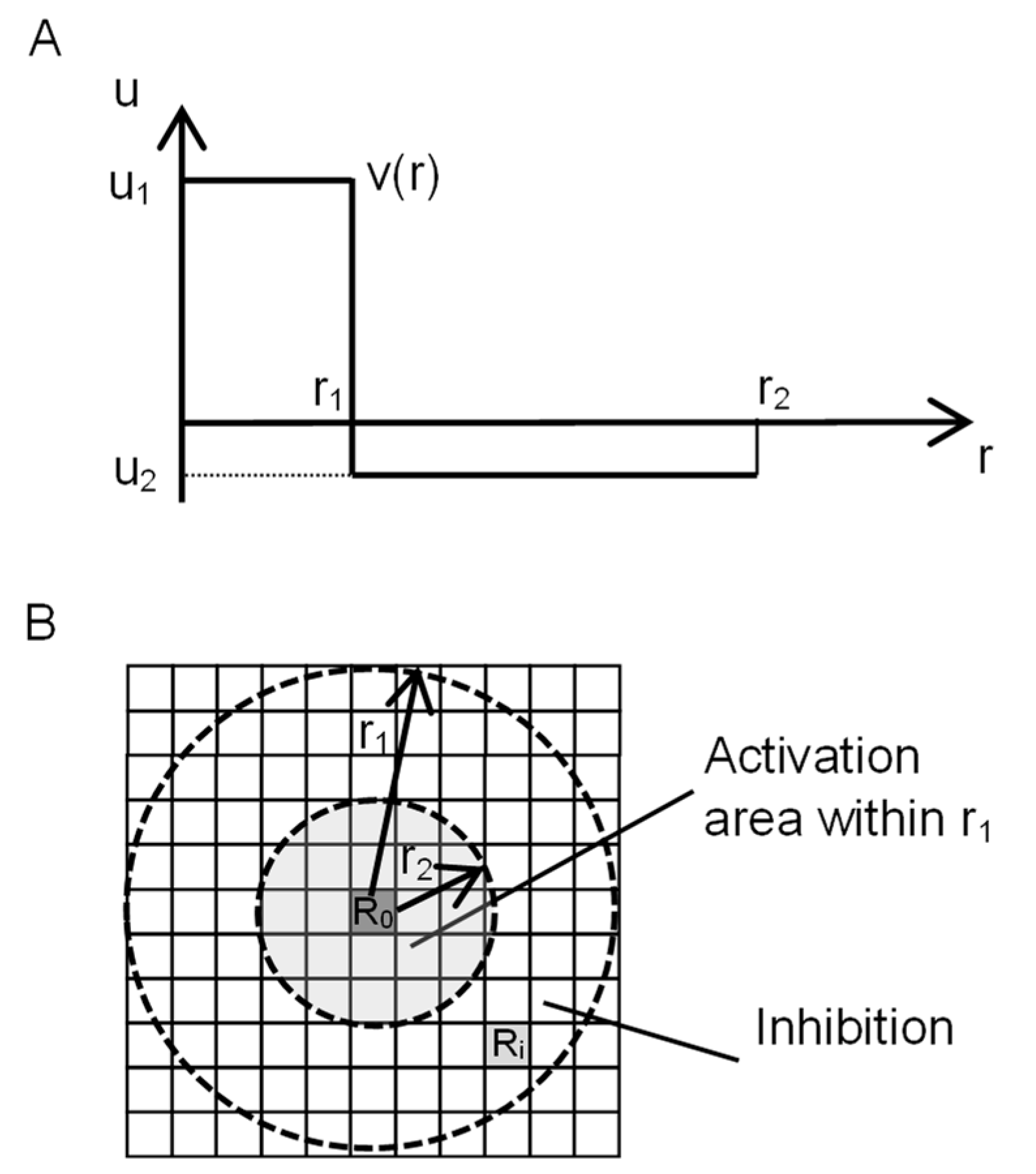
Young’s CA model [43] uses a real number function, v(r), to derive the distance effects, with two constant values within a grid cell—u₁ (positive) and u₂ (negative)—as shown in Figure 2A. The v(r) function is a step function. The activation area, indicated by u₁, has a radius of r₁; the inhibition area, indicated by u₂, has a radius of r₂ (r₂ > r₁) (Figure 2B). It is believed that Young’s model incorporates diffusion coefficient differences and nonlinear interactions using a step function. The calculation begins by distributing black cells randomly on a rectangular grid. Subsequently, for each cell at position R₀ in 2D fields, the next cell state of R₀ is determined by the value of function v(r). When R_i is assumed to be a black cell within radius r₂ from the R₀ cell and function |R₀ − R_i| is assumed to be the distance between R₀ and R_i, the next cell state of R₀ is determined by the sum of the function v (|R₀ − R_i|) value at all nearby black R_i cells. If ∑_i v (|R₀ − R_i|) > 0, the grid cell at point R₀ is marked as a black cell; in turn, if ∑_i v (|R₀ − R_i|) < 0, the grid cell becomes a white cell. Finally, if ∑_i v (|R₀ − R_i|) = 0, the grid cell does not change state [43]. Young reported that a Turing pattern can be generated using these functions. Spotted patterns or striped patterns can be created with relative changes between u₁ and u₂.

In the present study, the method of Ishida was used [48], who converted Young’s model into a simpler CA model. Ishida’s method can be described as follows. In this Young’s model, let u₁ = 1 and u₂ = w (here, 0 < w < 1); furthermore, if the state of the cell is set to 0 (white) and 1 (black), this model can be arranged as follows. The state of cell i is expressed as c_i(t) (c_i(t) = [0, 1]) at time t. The subsequent state at time t + 1, c_i(t + 1), is determined by the states of the neighboring cells. Here, N₁ is the sum of the states of the domain within the S₁ meshes of the focal cell. Similarly, N₂ is the sum of the states of the domain within the S₂ meshes of the focal cell, assuming that S₁ < S₂.

$$N_1=\sum _{i=1}^{S_1}{c}_i\left(t\right)$$

$$N_2=\sum _{i=1}^{S_2}{c}_i\left(t\right),$$

where S₁ and S₂ are the numbers of cells within the S₁ and S₂ meshes of the focal cell. In addition, S₂ = 2S₁ was assumed in this paper. Figure 3 provides a schematic representation of the total sum of states N₁ and N₂. The next state of the focal cell is determined by the following expression (1):

$$\mathrm{C}\mathrm{e}\mathrm{l}\mathrm{l}\mathrm{s}\mathrm{t}\mathrm{a}\mathrm{t}\mathrm{e}\mathrm{a}\mathrm{t}\mathrm{t}\mathrm{h}\mathrm{e}\mathrm{n}\mathrm{e}\mathrm{x}\mathrm{t}\mathrm{t}\mathrm{i}\mathrm{m}\mathrm{e}\mathrm{s}\mathrm{t}\mathrm{e}\mathrm{p}=\left\{\begin{array}{c}1:\mathrm{if}{(N}_1-N_2\mathrm{w})>0\\ \mathrm{Unchange}:\mathrm{if}{(N}_1-N_2\mathrm{w})=0\\ 0:\mathrm{if}{(N}_1-N_2\mathrm{w})<0\end{array}\right.,$$

(1)

where w and S₁ are the two parameters that determine the Turing pattern.

2.3. Majority Voting Model Using CA

Here, a model that applied the majority decision model proposed by Vichniac was considered [39]. The Vichniac model is a cellular automaton model that uses the sum rule of Moore neighborhoods (eight adjacent cells); however, in this model, cells in the S₁ range described in the previous section were considered, rather than cells that were merely adjacent. The focal cell value was set to 1 if the sum of the states in the cells in this S₁ range was greater than half the number of cells in the S₁ range and to 0 if the sum was less than that. If the cell space was bisected by a straight line into black and white, and if this model was considered to be on the boundary, exactly half of black and white would be obtained. Cells slightly on the white side of the boundary would be whiter, whereas cells slightly on the black side would be blacker. Therefore, if the initial value was in such an arrangement, the pattern would not change when this model is applied. Conversely, if black and white were randomly arranged as initial values, unevenness in the ratio of black to white would occur in the local space, and a pattern using this as the seed would arise. The results of the time evolution from a random initial state performed using this model strongly depended on the ratio or distribution of 1s and 0s in the initial state. When given the appropriate initial ratio, it is possible to form patterns that resemble animal body patterns. The equation for the majority voting model in this study is indicated in (2):

$$\mathrm{C}\mathrm{e}\mathrm{l}\mathrm{l}\mathrm{s}\mathrm{t}\mathrm{a}\mathrm{t}\mathrm{e}\mathrm{a}\mathrm{t}\mathrm{t}\mathrm{h}\mathrm{e}\mathrm{n}\mathrm{e}\mathrm{x}\mathrm{t}\mathrm{t}\mathrm{i}\mathrm{m}\mathrm{e}\mathrm{s}\mathrm{t}\mathrm{e}\mathrm{p}=\left\{\begin{array}{c}1:\mathrm{if}{N}_1>\frac{N_0}{2}\\ \mathrm{Unchanged}:\mathrm{if}{N}_1=\frac{N_0}{2}\\ 0:\mathrm{if}{N}_1<\frac{N_0}{2}\end{array}\right.,$$

(2)

where N₁ is the sum of the states of the domain within the S₁ meshes of the focal cell and N₀ is the total number of cells within the S₁ range.

2.4. Proposed Integration Model

After the integration of the two models presented in Equations (1) and (2), they can be expressed using two parameters, w and a, by considering equations such as (3):

$$\mathrm{C}\mathrm{e}\mathrm{l}\mathrm{l}\mathrm{s}\mathrm{t}\mathrm{a}\mathrm{t}\mathrm{e}\mathrm{a}\mathrm{t}\mathrm{t}\mathrm{h}\mathrm{e}\mathrm{n}\mathrm{e}\mathrm{x}\mathrm{t}\mathrm{t}\mathrm{i}\mathrm{m}\mathrm{e}\mathrm{s}\mathrm{t}\mathrm{e}\mathrm{p}=\left\{\begin{array}{c}1:\mathrm{if}{(N}_1-N_2\mathrm{w})>\mathrm{a}\\ \mathrm{Unchanged}:\mathrm{if}{(N}_1-N_2\mathrm{w})=\mathrm{a}\\ 0:\mathrm{if}{(N}_1-N_2\mathrm{w})<\mathrm{a}\end{array}\right.$$

(3)

In (3), when w > 0 and a = 0, the equation becomes the same as Equation (1) and is a Turing pattern model. In turn, when w = 0 and a = N₀/2 in Equation (3), the model is equivalent to Equation (2) and is a majority rule model. It is also possible to construct a model that has intermediate parameters between the two models by varying w and a. This is the integrated model of the two models.

2.5. Model with Invariant Regions at the Boundary of the Patterns

A variant of the majority voting model reported by Vichniac [39] has also been proposed. At the pattern boundary, where the majority decision is divided, the model is deformed in that the sum of the Moore neighborhoods is 0 when it should be 1 if the sum value was 5, and it is 1 when it should be 0 if the sum value was 4. This model weakens the effect of the majority decision at the pattern’s boundary. Based on this, a model was also devised that does not follow the Turing model or the majority rule model for the boundary domain of the pattern. Equation (4) is a model with a range that is invariant at the boundary of the pattern:

$$\mathrm{C}\mathrm{e}\mathrm{l}\mathrm{l}\mathrm{s}\mathrm{t}\mathrm{a}\mathrm{t}\mathrm{e}\mathrm{a}\mathrm{t}\mathrm{t}\mathrm{h}\mathrm{e}\mathrm{n}\mathrm{e}\mathrm{x}\mathrm{t}\mathrm{t}\mathrm{i}\mathrm{m}\mathrm{e}\mathrm{s}\mathrm{t}\mathrm{e}\mathrm{p}=\left\{\begin{array}{c}1:\mathrm{if}{(N}_1-N_2\mathrm{w})>\mathrm{a}(1+\mathrm{b})\\ 0:\mathrm{if}{(N}_1-N_2\mathrm{w})<\mathrm{a}\left(1-\mathrm{b}\right)\\ \mathrm{Unchanged}:\mathrm{otherwise}\end{array}\right.$$

(4)

Here, a new parameter, b, has been added to set the range of the unchanged region.

2.6. Calculation Conditions

The model used 2D hexagonal grids (Figure 4) in which the application of transition rules was simple. Although square grids are generally used in 2D CA modeling, it also used hexagonal grids because they are isotropic compared to a square grid. The calculation program was implemented in JavaScript and can run on various browsers. Each step could be executed within 1 s on a personal computer (Windows 10, Intel Core i7). If there is no change in the result from the previous time step, it is determined that the process has converged. Although differences exist depending on the calculation conditions, they generally converge within 30 time steps.

The models were implemented using the following conditions:

-

Calculation field: 100 × 100 cells in a hexagonal grid;

-

Periodic boundary condition;

-

Initial conditions: states 0 and 1 were placed randomly in each cell of the computational field with a probability of 0.5;

-

At each time step, the cells in the lattice space were synchronously changed, and the computation was repeated until the pattern formation stabilized;

-

The range of S₁ was set to three cells from the focal cell, and the range of S₂ was set to six cells from the focal cell. The parameter s determines the scale of the pattern to be created and, if it is larger, the patterns will only become more similar and larger. For this reason, s was fixed.

3. Results

3.1. Parameter Map

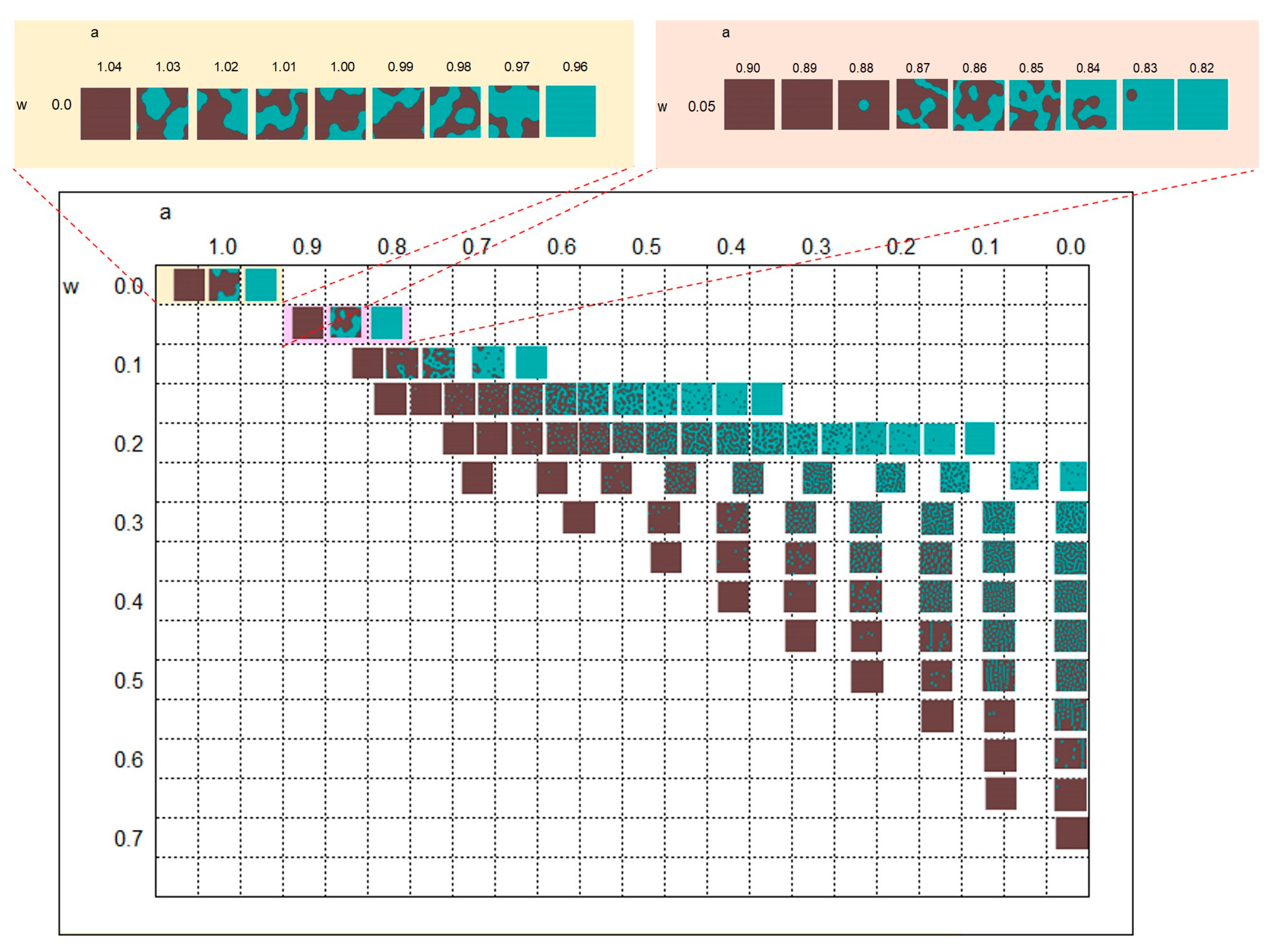
In the integrated model, after setting each parameter of w and a, the calculation was initiated from random initial values until the pattern became stationary. Figure 5 shows the parameter map, where the black cells indicate state 0 and the blue cells indicate state 1.

The results of w = 0 and a = 1.0 at the top of the figure were equivalent to those of the majority voting model. In the case of the majority voting model with w = 0, the results changed sensitively according to the value of a. Therefore, the upper part of the entire map shows the results obtained when parameter a was altered slightly. When parameter a exceeded 1.0, the entire image was black (0), whereas when parameter a was <1.0, the entire image was blue (1).

The result of changing w with a = 0 in the rightmost column of the figure was equivalent to that of the Turing model. In regions where the w value was small, the cells were indicated in blue. As the w value increased, the cells appeared as black spots, changed to a striped pattern, became a blue-speckled pattern, and finally became fully black. These results are consistent with those of Ishida [48] and it is believed that the Turing pattern was reproduced.

The result of changing parameter a with each w value show that the patterns were all black when the value of a was large. As the value of a decreased, the patterns became similar to those of the Turing pattern model with a = 0. It could also be observed that the effect of the majority voting model was stronger at approximately w = 0.1.

3.2. Initial Value Dependency

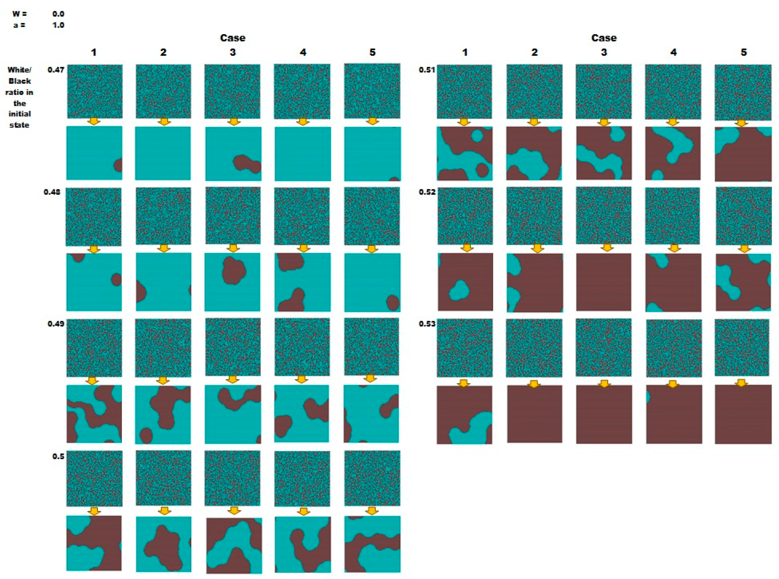
Smaller values of the parameter w (closer to the majority model) showed higher dependency on the initial value. Figure 6 presents the results of the initial value’s dependence in the equivalent model of majority voting with w = 0.0 and a = 1.0. These results were obtained when the cell states were placed randomly according to the specified black (0)/blue (1) ratio as the initial value. These are the results of five calculations at each ratio.

The results of this analysis revealed that a slight change in the initial value of the black/blue ratio (from 0.47 to 0.53) significantly changed the black and blue composition of the final pattern. Moreover, for the same black/blue ratio, the compositions of black and blue patterns in the final pattern tended to be similar, although the patterns changed for each calculation. The majority voting model with a black/blue ratio of 0.5 produced a pattern similar to the striped pattern.

3.3. Results of the Model with Invariant Regions at the Boundary of the Patterns

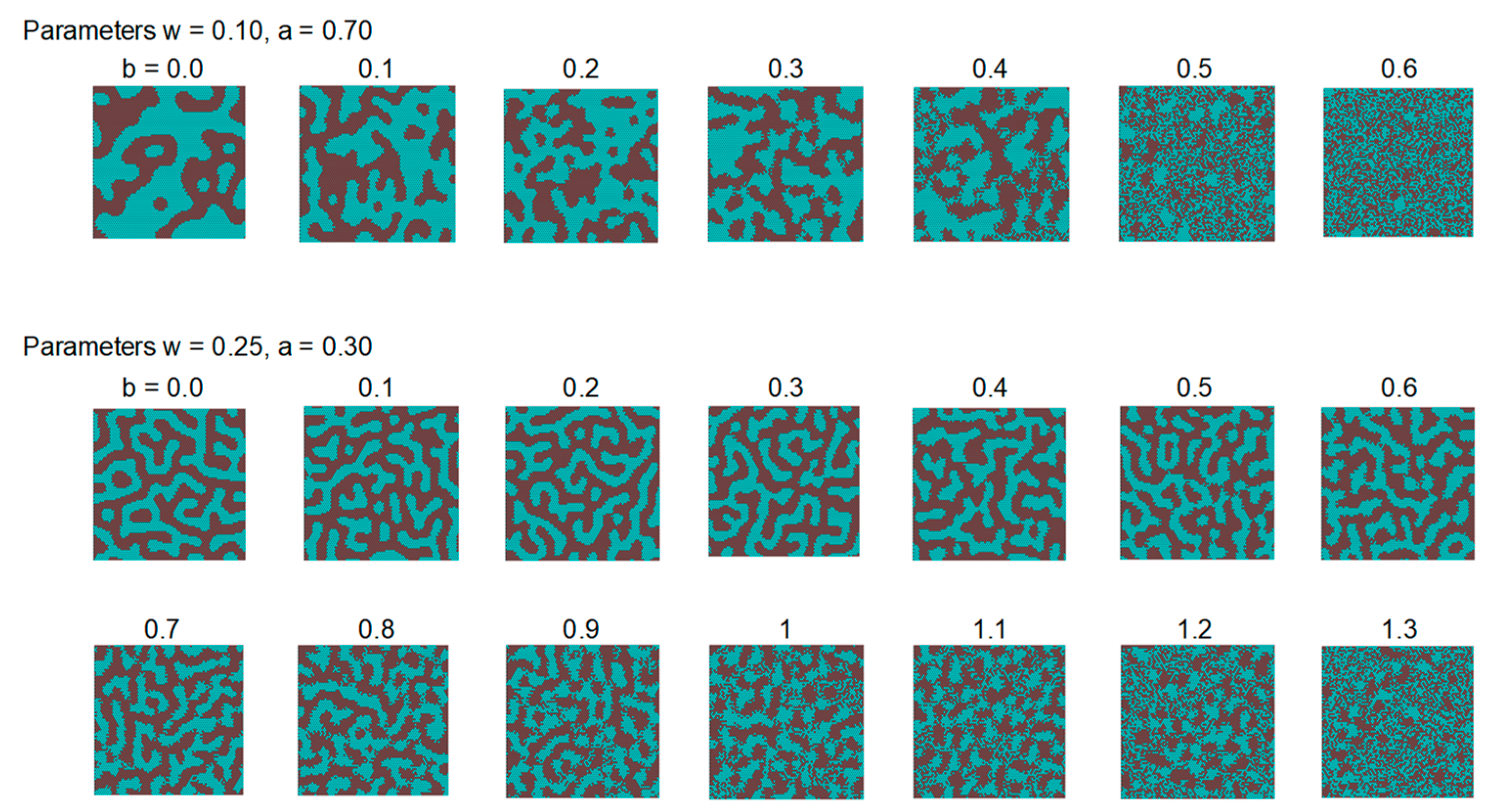
Figure 7 shows the results of the model that included regions in which the state was invariant at the boundaries of the patterns. The figure depicts the results obtained when b was altered under fixed conditions of the parameters w and a. In this model, a larger value of parameter b yielded a larger region in which the state that remained unchanged near the boundary of the pattern may expand. The results showed that the boundary of the pattern became more ambiguous as b increased.

4. Discussion

In this integrated model, when parameter w was 0, the model was assessed via a majority vote of the states of nearby cells. In contrast, when w was different from 0, the model tended to invert and incorporate the intensity of the information from distant locations (as indicated by the formula N₁ − N₂ × w, where N₂ at distant locations was negatively affected), thus creating a Turing pattern.

In particular, in the case of varying w when a = 0, the parameter w, which varies the Turing pattern, is a weight coefficient that adjusts the magnitude of the effect of the number of states in the outer neighborhood (N₂) on the number of states in the inner neighborhood (N₁). At the rightmost portion of Figure 5, a typical Turing pattern appears as the w value changes. In the RD model, this w value corresponds to the difference between the diffusion coefficients of the two diffuse substances and corresponds to the result in which the pattern is created by the difference between the two diffusion coefficients.

In Figure 5, when w = 2.0 is fixed and parameter a is varied, a continuous pattern that changes from a speckled pattern to a striped pattern similar to the Turing pattern can be observed. This indicates that, under constant w value conditions (w = 0.2 in this case), a change in parameter a can induce the same pattern change as a change in the w value. In equation $N_1-N_2\times \mathrm{w}>\mathrm{a}·\frac{N_0}{2}$, parameter w is the parameter for adjusting the difference between N₁ and N₂. However, even when w is fixed in a certain range and a is varied, the value of a can affect the magnitude of the difference between N₁ and N₂. The condition of w being fixed means that, although the difference in diffusion coefficients between the two substances is fixed, the pattern can be changed by looking at the value of the difference in a diffusion concentration under certain conditions. This suggests that the model can be converted into a simpler mechanism for pattern creation than the conventional model, which requires detailed changes in the diffusion coefficient to change the pattern and may provide useful knowledge for exploring the mechanism in vivo.

In Figure 7, parameter b has the effect of blurring the boundary of the pattern and reflecting random initial conditions in the boundary region. Although this model is a deterministic state transition model, when near the boundary of the pattern (a region where the effects of the inner and outer neighborhoods are antagonistic), the model could transform into a model with a stochastic transition to 0 or 1. Although the model and results of this study alone do not clarify how these parameters relate to specific mechanisms within the organism, the simplicity of this model may be helpful in future studies of these in vivo models.

For example, the process of counting the number of states in the surrounding cells in the model could correspond to the process by which cells receive signaling substances, such as proteins, from neighboring cells. Furthermore, the transition between blue and black cells could correspond to signals controlling chromatophores in pigment cells, a phenomenon which could facilitate the understanding of the regulatory mechanism for skin patterns.

The following are the results from a comparative study of these results using actual biological patterns. Figure 8 displays the results of the majority voting model. The fact that large patterns are formed at any initial value, despite being sensitive to the initial value, may explain the formation of Nishiki goi patterns. In general, a fixed number of colors are observed in Nishiki goi patterns; however, the appearance of the patterns varies greatly among individuals. This may explain why Nishiki goi patterns vary with slight changes in the conditions in the epidermal cells during the growth process, corresponding to the initial value dependence of the model.

Figure 8 indicates the results obtained using parameters that were intermediate between those of the majority rule model and the Turing model, showing that patterns created using this approach could not be generated using the Turing model. The image on the right in Figure 8 provides an example of the pattern of the pufferfish Takifugu vermicularis which is similar to the resulting pattern produced by the present model. Thus, a model with intermediate parameter values could reproduce a wide variety of fish patterns.

Figure 8 provides an example of the calculation results based on a model in which the state was invariant in the boundary region of the patterns. A pattern in which the boundaries of the pattern are intermittently connected could be created, as observed in the case of the pufferfish Takifugu stictonotus.

Figure 8 depicts a speckled pattern with a typical Turing pattern. Under these conditions, it can be assumed that the pattern of the pufferfish Takifugu alboplumbeus was reproduced. In the pufferfish family, the patterns vary greatly from species to species [6]; however, using this model, it was possible to create patterns in the same model by adjusting the parameters.

Thus, in addition to the effects of short-range activation and long-range inhibition, the proposed model can generate numerous patterns by considering the mechanism of the majority voting model and the stochastic transformation of pattern boundaries.

In addition, the proposed model formed patterns by counting the states of the surrounding neighboring cells. It is a model that can be computed only via information transfer from neighboring cells. Therefore, it is possible to construct a model that corresponds to the recent experimental results of Turing patterns, such as mutual stimulation between cells. Although this model is simpler than the conventional computational models, it has the potential to create a wide variety of patterns. Conversely, alternative mechanisms of pattern formation without the Turing instability have been proposed [49], and their consistency with these models should be examined in the future.

Analyses of the overall parameter map (Figure 5) revealed that most of the map area was all black, i.e., an area that did not create patterns. This is consistent with the trend reported by Miyazawa [36] in which most fish had no pattern. Patterns are created exclusively when certain combinations of parameters are used. In particular, the patterns of Nishiki goi emerged only in an extremely narrow region of parameter a, under the condition of w = 0.0. Creating such a pattern is believed to be difficult under natural selection; these patterns can be explained by consistent artificial selection over a long period of time. Future studies should also address the pattern stability issues and the robustness of the proposed model, as previously investigated by Maini et al. [50].

5. Conclusions

In this study, the Turing pattern and majority voting models were represented using a CA, resulting in the proposal of a model that integrated these two models. By adjusting the parameters, this integrated model could create patterns that are equivalent to both previously mentioned models. By setting the intermediate parameter values of the two models, it was possible to create a variety of patterns that were more diverse than those created by each model alone. Although this model is simpler than previously proposed models, it can create a variety of patterns. However, further research is warranted to determine whether this model is consistent with the mechanisms involved in the formation of skin patterns in fish from a biological viewpoint. Furthermore, a quantitative evaluation of pattern formation is required—especially the use of pattern simplicity scores or pair correlation functions—to understand the wavelengths that appear in the patterns and the variation caused by initial conditions. Although the model developed in this study alone cannot further elucidate the in vivo mechanism, a biochemical model equivalent to the formula for determining two colors might reveal a different candidate substance for morphogenesis. When speculating on extending this integrated model to three colors, the possibility that the three-color pattern might be potentially due to two or more overlapping and independent mechanisms should be considered as well.

In fact, many fish species dynamically change their patterns during the growth and maturation process from the juvenile to the adult stage. A possible explanation for this finding is that cell–cell interactions on the epidermis change as the fish grows. It is believed that the application of this model may allow the examination of large-scale changes in patterns associated with growth.

References

1. Turing, A.M. The chemical basis of morphogenesis. Phil. Trans. R. Soc. Lond. B 1952, 237, 37–72. [Google Scholar]
2. Meinhardt, H. Models of Biological Pattern Formation; Academic Press: New York, NY, USA, 1982; Volume 6. [Google Scholar]
3. Wolpert, L. Positional information and the spatial pattern of cellular differentiation. J. Theor. Biol. 1969, 25, 1–47. [Google Scholar] [CrossRef] [PubMed]
4. Wolpert, L. Positional information revisited. Development 1989, 107 (Suppl. S3), 3–12. [Google Scholar] [CrossRef] [PubMed]
5. Kondo, S.; Asal, R. A reaction-diffusion wave on the skin of the marine angelfish Pomacanthus. Nature 1995, 376, 765–768. [Google Scholar] [CrossRef] [PubMed]
6. Miyazawa, S.; Okamoto, M.; Kondo, S. Blending of animal colour patterns by hybridization. Nat. Commun. 2010, 1, 66. [Google Scholar] [CrossRef] [PubMed]
7. Milinkovitch, M.C.; Jahanbakhsh, E.; Zakany, S. The unreasonable effectiveness of reaction diffusion in vertebrate skin color patterning. Annu. Rev. Cell Dev. Biol. 2023, 39, 145–174. [Google Scholar] [CrossRef] [PubMed]
8. Entchev, E.V.; Schwabedissen, A.; González-Gaitán, M. Gradient formation of the TGF-beta homolog Dpp. Cell 2000, 103, 981–991. [Google Scholar] [CrossRef] [PubMed]
9. Sick, S.; Reinker, S.; Timmer, J.; Schlake, T. WNT and DKK determine hair follicle spacing through a reaction-diffusion mechanism. Science 2006, 314, 1447–1450. [Google Scholar] [CrossRef] [PubMed]
10. Economou, A.D.; Ohazama, A.; Porntaveetus, T.; Sharpe, P.T.; Kondo, S.; Basson, M.A.; Gritli-Linde, A.; Cobourne, M.T.; Green, J.B.A. Periodic stripe formation by a Turing mechanism operating at growth zones in the mammalian palate. Nat. Genet. 2012, 44, 348–351. [Google Scholar] [CrossRef]
11. Dilão, R.; Muraro, D. mRNA diffusion explains protein gradients in Drosophila early development. J. Theor. Biol. 2010, 264, 847–853. [Google Scholar] [CrossRef]
12. Dilão, R. Bicoid mRNA diffusion as a mechanism of morphogenesis in Drosophila early development. Comptes Rendus Biol. 2014, 337, 679–682. [Google Scholar] [CrossRef]
13. Yamaguchi, M.; Yoshimoto, E.; Kondo, S. Pattern regulation in the stripe of zebrafish suggests an underlying dynamic and autonomous mechanism. Proc. Natl. Acad. Sci. USA 2007, 104, 4790–4793. [Google Scholar] [CrossRef]
14. Nakamasu, A.; Takahashi, G.; Kanbe, A.; Kondo, S. Interactions between zebrafish pigment cells responsible for the generation of Turing patterns. Proc. Natl. Acad. Sci. USA 2009, 106, 8429–8434. [Google Scholar] [CrossRef]
15. Frohnhöfer, H.G.; Krauss, J.; Maischein, H.M.; Nüsslein-Volhard, C. Iridophores and their interactions with other chromatophores are required for stripe formation in zebrafish. Development 2013, 140, 2997–3007. [Google Scholar] [CrossRef]
16. Woolley, T.E. Pattern production through a chiral chasing mechanism. Phys. Rev. E 2017, 96, 032401. [Google Scholar] [CrossRef]
17. Yamanaka, H.; Kondo, S. In vitro analysis suggests that difference in cell movement during direct interaction can generate various pigment patterns in vivo. Proc. Natl. Acad. Sci. USA 2014, 111, 1867–1872. [Google Scholar] [CrossRef]
18. Inaba, M.; Yamanaka, H.; Kondo, S. Pigment pattern formation by contact-dependent depolarization. Science 2012, 335, 677. [Google Scholar] [CrossRef]
19. Hamada, H.; Watanabe, M.; Lau, H.E.; Nishida, T.; Hasegawa, T.; Parichy, D.M.; Kondo, S. Involvement of Delta/Notch signaling in zebrafish adult pigment stripe patterning. Development 2014, 141, 318–324. [Google Scholar] [CrossRef]
20. Kondo, S.; Watanabe, M.; Miyazawa, S. Studies of Turing pattern formation in zebrafish skin. Philos. Trans. A Math. Phys. Eng. Sci. 2021, 379, 20200274. [Google Scholar] [CrossRef]
21. Watanabe, M.; Kondo, S. Is pigment patterning in fish skin determined by the Turing mechanism? Trends Genet. 2015, 31, 88–96. [Google Scholar] [CrossRef]
22. Bullara, D.; De Decker, Y. Pigment cell movement is not required for generation of Turing patterns in zebrafish skin. Nat. Commun. 2015, 6, 6971. [Google Scholar] [CrossRef]
23. Caicedo-Carvajal, C.E.; Shinbrot, T. In silico zebrafish pattern formation. Dev. Biol. 2008, 315, 397–403. [Google Scholar] [CrossRef]
24. Volkening, A.; Sandstede, B. Modelling stripe formation in zebrafish: An agent-based approach. J. R. Soc. Interface 2015, 12, 20150812. [Google Scholar] [CrossRef]
25. Volkening, A.; Sandstede, B. Iridophores as a source of robustness in zebrafish stripes and variability in Danio patterns. Nat. Commun. 2018, 9, 3231. [Google Scholar] [CrossRef]
26. Vasilopoulos, G.; Painter, K.J. Pattern formation in discrete cell tissues under long range filopodia-based direct cell to cell contact. Math. Biosci. 2016, 273, 1–15. [Google Scholar] [CrossRef]
27. Marcon, L.; Diego, X.; Sharpe, J.; Müller, P. High-throughput mathematical analysis identifies Turing networks for patterning with equally diffusing signals. eLife 2016, 5, e14022. [Google Scholar] [CrossRef]
28. Moreira, J.; Deutsch, A. Pigment pattern formation in zebrafish during late larval stages: A model based on local interactions. Dev. Dyn. 2005, 232, 33–42. [Google Scholar] [CrossRef]
29. Konow, C.; Li, Z.; Shepherd, S.; Bullara, D.; Epstein, I.R. Influence of survival, promotion, and growth on pattern formation in zebrafish skin. Sci. Rep. 2021, 11, 9864. [Google Scholar] [CrossRef]
30. Owen, J.P.; Kelsh, R.N.; Yates, C.A. A quantitative modelling approach to zebrafish pigment pattern formation. eLife 2020, 9, e52998. [Google Scholar] [CrossRef]
31. Ishida, T.; Tadokoro, H.; Takahashi, H.; Yoshikawa, H.; Harumi, S. Constructing models to reproduce the skin color patterns of Takifugu species, including hybrids, fisheries. Engineering 2019, 15, 15–26. [Google Scholar]
32. Zakany, S.; Smirnov, S.; Milinkovitch, M.C. Lizard skin patterns and the Ising model. Phys. Rev. Lett. 2022, 128, 048102. [Google Scholar] [CrossRef]
33. Graner, F.; Glazier, J.A. Simulation of biological cell sorting using a two-dimensional extended Potts model. Phys. Rev. Lett. 1992, 69, 2013–2016. [Google Scholar] [CrossRef]
34. Dilão, R.; Sainhas, J. Modelling butterfly wing eyespot patterns. Proc. Biol. Sci. 2004, 271, 1565–1569. [Google Scholar] [CrossRef] [PubMed]
35. Kondo, S. An updated kernel-based Turing model for studying the mechanisms of biological pattern formation. J. Theor. Biol. 2017, 414, 120–127. [Google Scholar] [CrossRef]
36. Miyazawa, S. Pattern blending enriches the diversity of animal colorations. Sci. Adv. 2020, 6, eabb9107. [Google Scholar] [CrossRef] [PubMed]
37. Jiang, Y.; Zhang, S.; Xu, J.; Feng, J.; Mahboob, S.; Al-Ghanim, K.A.; Sun, X.; Xu, P. Comparative transcriptome analysis reveals the genetic basis of skin color variation in common carp. PLoS ONE 2014, 9, e108200. [Google Scholar] [CrossRef]
38. Qiu, J. Epigenetics: Unfinished symphony. Nature 2006, 441, 143–145. [Google Scholar] [CrossRef]
39. Vichniac, G.Y. Simulating physics with cellular automata. Phys. D Nonlinear Phenom. 1984, 10, 96–116. [Google Scholar] [CrossRef]
40. Gierer, A.; Meinhardt, H.A. A Theory of biological pattern formation. Kybernetik 1972, 12, 30–39. [Google Scholar] [CrossRef]
41. Gray, P.; Scott, S. Autocatalytic reactions in the isothermal continuous stirred tank reactor. Chem. Eng. Sci. 1983, 38, 29–43. [Google Scholar] [CrossRef]
42. Schepers, H.E.; Markus, M. Two types of performance of an isotropic cellular automaton: Stationary (Turing) patterns and spiral waves. Physica A 1992, 188, 337–343. [Google Scholar] [CrossRef]
43. Young, D.A.A. A Local activator-inhibitor model of vertebrate skin patterns. Math. Biosci. 1984, 72, 51–58. [Google Scholar] [CrossRef]
44. Adamatzky, A.; Martínez, G.J.; Mora, J.C.S.T. Phenomenology of reaction-diffusion binary-state cellular automata. Int. J. Bifürcation Chaos 2006, 16, 2985–3005. [Google Scholar] [CrossRef]
45. Dormann, S.; Deutsch, A.; Lawniczak, A.T. Fourier analysis of turing-like pattern formation in cellular automaton models. Future Gen. Comp. Syst. 2001, 17, 901–909. [Google Scholar] [CrossRef]
46. Tsai, L.L.; Hutchison, G.R.; Peacock-López, E. Turing patterns in a self-replicating mechanism with a self-complementary template. J. Chem. Phys. 2000, 113, 2003–2006. [Google Scholar] [CrossRef]
47. Manukyan, L.; Montandon, S.A.; Fofonjka, A.; Smirnov, S.; Milinkovitch, M.C. A living mesoscopic cellular automaton made of skin scales. Nature 2017, 544, 173–179. [Google Scholar] [CrossRef]
48. Ishida, T. Possibility of controlling self-organized patterns with totalistic cellular automata consisting of both rules like game of life and rules producing Turing patterns. Micromachines 2018, 9, 339. [Google Scholar] [CrossRef]
49. Guisoni, N.; Diambra, L. Transient Turing patterns in a morphogenetic model. Front. Phys. 2022, 10, 927152. [Google Scholar] [CrossRef]
50. Maini, P.K.; Woolley, T.E.; Baker, R.E.; Gaffney, E.A.; Lee, S.S. Turing’s model for biological pattern formation and the robustness problem. Interface Focus. 2012, 2, 487–496. [Google Scholar] [CrossRef]
Figure 1. Examples of Nishiki goi patterns. (A) Nishiki goi is an ornamental carp (Cyprinus carpio) in which various patterns have been created via crossbreeding, including two-color red and white patterns and three-color white, red, and black patterns. (B) Examples of two-color Nishiki goi patterns with red and white patterns. (C) Examples of three-color Nishiki goi patterns with white, red, and black patterns.
Biophysica 04 00020 g001
Figure 2. Outline of Young’s model. (A) Function v(r) is a continuous step function representing the activation area and the inhibition area. (B) The activation area has a radius indicated by r1, and the inhibition area has an outer radius indicated by r2.
Biophysica 04 00020 g002
Figure 3. Schematic representation of the summing of states N1 and N2. Each grid cell has a 0 (white) or 1 (black) state. The inner area has a domain within the s grids of the focal cell (pink color cell), and the outer area has a domain within the 2s grids.
Biophysica 04 00020 g003
Figure 4. Hexagonal grid field. Here, N1 is the domain within the S1 meshes of the focal cell. Similarly, N2 is the sum of the states of the domain within the S2 meshes of the focal cell, assuming that S1 < S2.
Biophysica 04 00020 g004
Figure 5. Parameter map with parameters w and a; the black cells indicate a state of 0, and the blue cells indicate a state of 1. The results obtained for w = 0 and a = 1.0 indicated at the top of the figure were equivalent to those of the majority voting model. In the case of the majority voting model with w = 0, the results changed sensitively according to the value of a. Therefore, the upper part of the whole map presents the results obtained when a was varied slightly. The result obtained by changing the w value with a = 0 in the rightmost column of the figure was equivalent to that of the Turing model.
Biophysica 04 00020 g005
Figure 6. Dependence of the initial values in the majority voting model. These are the results of five calculations at each black (0)/blue (1) ratio as the initial value. The results indicate that a slight change in the black/blue ratio (from 0.47 to 0.53) as the initial value can significantly change the black and blue composition of the final pattern.
Biophysica 04 00020 g006
Figure 7. Results of the model with invariant regions at the boundary of the patterns; parameter b indicates the range of the unchanged range on the pattern’s edge, with a larger parameter b yielding a larger region in which the state that remained unchanged near the boundary of the pattern may expand. The results show that the boundary of the pattern became more ambiguous as b increased.
Biophysica 04 00020 g007
Figure 8. Comparison of the calculation results from the integrated model with the actual patterns of the fish. It was found that the proposed integrated model created a variety of patterns, from seemingly random patterns (such as those of Nishiki goi) to typical Turing model patterns, using a single model. 1 Web Fish Encyclopedia; https://zukan.com/media/leaf/original/41224.jpg (accessed on 26 March 2024).
Biophysica 04 00020 g008
Disclaimer/Publisher’s Note: The statements, opinions and data contained in all publications are solely those of the individual author(s) and contributor(s) and not of MDPI and/or the editor(s). MDPI and/or the editor(s) disclaim responsibility for any injury to people or property resulting from any ideas, methods, instructions or products referred to in the content.