
Search for Entanglement between Spatially Separated Living Systems: Experiment Design, Results, and Lessons Learned

 , , , and
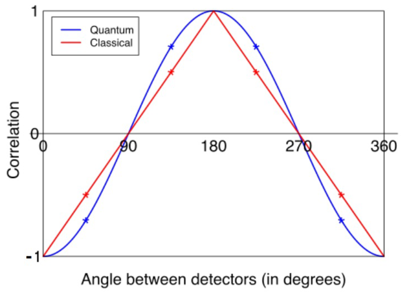
Abstract
1. Introduction
2. Materials and Methods
2.1. General Structure of CHSH Tests
2.2. Design of the Present Experiment
2.3. Cell Biology Methods
2.4. EEG Methods
2.5. HRV and GSR Methods
2.6. Statistical Methods
- ANOVA over four periods (1 × 4 design): Pre-Baseline, Post-Baseline, Treatment 1, and Treatment 3;
- Paired t-test (1 × 2 design): Treatment 1 and 3 combined versus Pre- and Post-Baselines combined;
- Paired t-test (1 × 2 design): Treatment 1 versus Pre- and Post-periods combined (1 × 2 design);
- Paired t-test (1 × 2 design): Treatment 1 versus Treatment 2;
- Two-way ANOVA (2 × 2 design): Treatment 1 and 3 combined versus Pre- and Post-Baseline combined and cells of type 5 vs. cells of type 4 and 6 combined (cell types 4, 5, and 6 are blinded indices for live cells, cell-free media, and dead cells, in this or a permuted order).
3. Results
4. Discussion
5. Conclusions
Author Contributions
Funding
Institutional Review Board Statement
Informed Consent Statement
Data Availability Statement
Acknowledgments
Conflicts of Interest
Abbreviations
| BT | Biofield Therapy |
| CHSH | Clauser–Horne–Shimony-Holt |
| EEG | Electro-Encephalography |
| ER | Einstein–Rosen |
| EPR | Einstein–Podolsky–Rosen |
| GSR | Galvanic Skin Response |
| HRV | Heart Rate Variability |
| MEG | Magneto-Encephalography |
| NMR | Nuclear Magnetic Resonance |
| OR | Objective Reduction |
References
- Aspect, A.; Dalibard, J.; Roger, G. Experimental test of Bell’s inequaties using time-varying analyzers. Phys. Rev. Lett. 1982, 49, 1804–1807. [Google Scholar] [CrossRef]
- Horodecki, R.; Horodecki, P.; Horodecki, M.; Horodecki, K. Quantum entanglement. Rev. Mod. Phys. 2009, 81, 865–942. [Google Scholar] [CrossRef]
- Georgescu, I. How the Bell tests changed quantum physics. Nat. Phys. 2021, 3, 374–376. [Google Scholar] [CrossRef]
- Nielsen, M.A.; Chuang, I.L. Quantum Computation and Quantum Information; Cambridge University Press: Cambridge, UK, 2000. [Google Scholar]
- Dowling, J.P.; Milburn, G.J. Quantum technology: The second quantum revolution. Phil. Trans. R. Soc. Lond. A 2003, 361, 1655–1674. [Google Scholar] [CrossRef]
- Ladd, T.D.; Jelezko, F.; Laflamme, R.; Nakamura, Y.; Monroe, C.; O’Brien, J.L. Quantum computers. Nature 2010, 464, 45–53. [Google Scholar] [CrossRef] [PubMed]
- Gyongyosi, L.; Imre, S. A survey on quantum computing technology. Comput. Sci. Rev. 2019, 31, 51–71. [Google Scholar] [CrossRef]
- Zanardi, P. Virtual quantum subsystems. Phys. Rev. Lett. 2001, 87, 077901. [Google Scholar] [CrossRef]
- Zanardi, P.; Lidar, D.A.; Lloyd, S. Quantum tensor product structures are observable-induced. Phys. Rev. Lett. 2004, 92, 060402. [Google Scholar] [CrossRef]
- de la Torre, A.C.; Goyeneche, D.; Leitao, L. Entanglement for all quantum states. Eur. J. Phys. 2010, 31, 325–332. [Google Scholar] [CrossRef]
- Harshman, N.L.; Ranade, K.S. Observables can be tailored to change the entanglement of any pure state. Phys. Rev. A 2011, 84, 012303. [Google Scholar] [CrossRef]
- Thirring, W.; Bertlmann, R.A.; Köhler, P.; Narnhofer, H. Entanglement or separability: The choice of how to factorize the algebra of a density matrix. Eur. Phys. J. D 2011, 64, 181–196. [Google Scholar] [CrossRef]
- van Raamsdonk, M. Building up spacetime with quantum entanglement. Gen. Relativ. Grav. 2011, 42, 23232329. [Google Scholar] [CrossRef]
- Almheiri, A.; Dong, X.; Harlow, D. Bulk locality and quantum error correction in AdS/CFT. J. High Energy Phys. 2015, 4, 133. [Google Scholar] [CrossRef]
- Swingle, B. Spacetime from entanglement. Annu. Rev. Condens. Matter Phys. 2018, 9, 345–358. [Google Scholar] [CrossRef]
- Bain, J. Spacetime as a quantum error correcting code? Stud. Hist. Phil. Sci. B 2020, 71, 26–36. [Google Scholar] [CrossRef]
- Addazi, A.; Chen, P.; Fabrocini, F.; Fields, C.; Greco, E.; Lulli, M.; Marcianò, A.; Pasechnik, R. Generalized holographic principle, gauge invariance and the emergence of gravity à la Wilczek. Front. Astron. Space Sci. 2021, 8, 563450. [Google Scholar] [CrossRef]
- Fields, C.; Glazebrook, J.F.; Marcianò, A. Communication protocols and quantum error-correcting codes from the perspective of topological quantum field theory. arXiv 2023, arXiv:2303.16461. [Google Scholar]
- Maldacena, J.; Susskind, L. Cool horizons for entangled black holes. Forschr. Physik 2013, 61, 781–811. [Google Scholar] [CrossRef]
- Dai, D.-C.; Minic, D.; Stojkovic, D.; Fu, C. Testing the ER = EPR conjecture. Phys. Rev. D 2022, 102, 066004. [Google Scholar] [CrossRef]
- Schrödinger, E. What Is Life? Cambridge University Press: Cambridge, UK, 1944. [Google Scholar]
- Tegmark, M. Importance of quantum decoherence in brain processes. Phys. Rev. E 2000, 61, 4194–4206. [Google Scholar] [CrossRef]
- Arndt, M.; Juffmann, T.; Vedral, V. Quantum physics meets biology. HFSP J. 2009, 3, 386–400. [Google Scholar] [CrossRef] [PubMed]
- Lambert, N.; Chen, Y.-N.; Cheng, Y.-C.; Li, C.-M.; Chen, G.-Y.; Nori, F. Quantum biology. Nat. Phys. 2012, 9, 10–18. [Google Scholar] [CrossRef]
- Melkikh, A.V.; Khrennikov, A. Nontrivial quantum and quantum-like effects in biosystems: Unsolved questions and paradoxes. Prog. Biophys. Mol. Biol. 2015, 119, 137–161. [Google Scholar] [CrossRef] [PubMed]
- Nordén, B. Quantum entanglement: Facts and fiction–how wrong was Einstein after all? Quart. Rev. Biophys. 2016, 49, e17. [Google Scholar] [CrossRef] [PubMed]
- Marais, A.; Adams, B.; Ringsmuth, A.K.; Ferretti, M.; Gruber, J.M.; Hendrikx, R.; Schuld, M.; Smith, S.L.; Sinaykiy, I.; Krüger, T.P.J.; et al. The future of quantum biology. J. R. Soc. Interface 2018, 15, 20180640. [Google Scholar] [CrossRef] [PubMed]
- Cao, J.; Cogdell, R.J.; Coker, D.F.; Duan, H.-G.; Hauer, J.; Kleinekathöfer, U.; Jansen, T.L.C.; Mančal, T.; Miiller, R.J.D.; Ogilvie, J.P.; et al. Quantum biology revisited. Sci. Adv. 2020, 6, eaaz4888. [Google Scholar] [CrossRef] [PubMed]
- Fields, C.; Levin, M. Metabolic limits on classical information processing by biological cells. BioSystems 2021, 209, 104513. [Google Scholar] [CrossRef] [PubMed]
- Lechelon, M.; Meriguet, Y.; Gori, M.; Ruffenach, S.; Nardecchia, I.; Floriani, E.; Coquillat, D.; Teppe, F.; Mailfert, S.; Marguet, D.; et al. Experimental evidence for long-distance electrodynamic intermolecular forces. Sci. Adv. 2022, 8, eabl5855. [Google Scholar] [CrossRef] [PubMed]
- Lee, K.S.; Tan, Y.P.; Nguyen, L.H.; Budoyo, R.P.; Park, K.H.; Hufnagel, C.; Yap, Y.S.; Møbjerg, N.; Vedral, V.; Paterek, T.; et al. Entanglement in a qubit-qubit-tardigrade system. New J. Phys. 2022, 24, 123024. [Google Scholar] [CrossRef]
- Hameroff, S.; Penrose, R. Orchestrated reduction of quantum coherence in brain microtubules: A model for consciousness. Math. Comput. Simul. 1996, 40, 453–480. [Google Scholar] [CrossRef]
- Hameroff, S.; Penrose, R. Consciousness in the universe: A review of the ‘OrchOR’ theory. Phys. Life Rev. 2014, 11, 39–78. [Google Scholar] [CrossRef]
- Kerskens, C.M.; López Pérez, D. Experimental indications of non-classical brain functions. J. Phys. Comms. 2022, 6, 105001. [Google Scholar] [CrossRef]
- von Neumann, J. Mathematische Grundlagen der Quantenmechanik; Springer: Berlin/Heidelberg, Germany, 1932. [Google Scholar]
- Bohr, N. Atomic Physics and Human Knowledge; Wiley: New York, NY, USA, 1958. [Google Scholar]
- Wigner, E.P. Remarks on the mind-body question. In The Scientist Speculates; Good, I.J., Ed.; Basic Books: New York, NY, USA, 1962; pp. 284–302. [Google Scholar]
- Penrose, R. The Emperor’s New Mind; Oxford University Press: Oxford, UK, 1989. [Google Scholar]
- Stapp, H.P. Quantum theory and the role of mind in nature. Found. Phys. 2001, 31, 1465–1499. [Google Scholar] [CrossRef]
- Orlov, Y.F. The wave logic of consciousness: A hypothesis. Int. J. Theor. Phys. 1982, 21, 37–53. [Google Scholar] [CrossRef]
- Yukalov, V.I.; Sornette, D. Scheme of thinking quantum systems. Laser Phys. Lett. 2009, 6, 833–839. [Google Scholar] [CrossRef][Green Version]
- Khrennikov, A. Quantum Bayesianism as the basis of general theory of decision-making. Phil. Trans. R. Soc. A 2016, 374, 20150245. [Google Scholar] [CrossRef] [PubMed]
- Pothos, E.M.; Busemeyer, J.R. Can quantum probability provide a new direction for cognitive modeling? Behav. Brain Sci. 2013, 36, 255–327. [Google Scholar] [CrossRef] [PubMed]
- Dzhafarov, E.N.; Zhang, R.; Kujala, J. Is there contextuality in behavioural and social systems? Phil. Trans. R. Soc. A 2016, 374, 20150099. [Google Scholar] [CrossRef] [PubMed]
- Bell, J.S. On the problem of hidden variables in quantum mechanics. Rev. Mod. Phys. 1966, 38, 447–452. [Google Scholar] [CrossRef]
- Kochen, S.; Specker, E.P. The problem of hidden variables in quantum mechanics. J. Math. Mech. 1967, 17, 59–87. [Google Scholar] [CrossRef]
- Mermin, N.D. Hidden variables and the two theorems of John Bell. Rev. Mod. Phys. 1993, 65, 803–815. [Google Scholar] [CrossRef]
- Dzhafarov, E.N.; Kujala, J.V. Context-content systems of random variables: The contextuality-by-default theory. J. Math. Psych. 2016, 74, 11–33. [Google Scholar] [CrossRef]
- Dzhafarov, E.N.; Kon, M. On universality of classical probability with contextually labeled random variables. J. Math. Psych. 2018, 85, 17–24. [Google Scholar] [CrossRef]
- Cervantes, V.H.; Dzhafarov, E.N. Snow Queen is evil and beautiful: Experimental evidence for probabilistic contextuality in human choices. Decision 2018, 5, 193–204. [Google Scholar] [CrossRef]
- Basieva, I.; Cervantes, V.H.; Dzhafarov, E.N.; Khrennikov, A. True contextuality beats direct influences in human decision making. J. Exp. Psych. 2019, 148, 1925–1937. [Google Scholar] [CrossRef]
- Jain, S.; Hammerschlag, R.; Mills, P.; Cohen, L.; Krieger, R.; Vietan, C.; Lutgendorf, S. Clinical studies of biofield therapies: Summary, methodological challenges, and recommendations. Glob. Adv. Health Med. 2015, 4, 58–66. [Google Scholar] [CrossRef]
- Bengston, W. A method used to train skeptical volunteers to heal in an experimental setting. J. Altern. Compl. Med. 2007, 13, 329–331. [Google Scholar] [CrossRef]
- Clauser, J.F.; Horne, M.A.; Shimony, A.; Holt, R.A. Proposed experiment to test local hidden-variable theories. Phys. Rev. Lett. 1969, 23, 880–884. [Google Scholar] [CrossRef]
- Yang, P.; Chakraborty, S.; Nguyen, P.; Cui, M.; Cusimano, A.; Wei, D.; Prinsloo, S.; Cohen, L. Biofield therapy suppressed the growth of human pancreatic cancer cells by modulation of cell cycle and cell voltage potentials (abstract). Cancer Res. 2022, 82 (Suppl. S12), 5382. [Google Scholar] [CrossRef]
- Yang, P.; Chakraborty, S.; Nguyen, P.; Deng, D.; Cusimano, A.; Wei, D.; Cohen, L. Biofield therapy suppressed invasion and metastases of human pancreatic cancer (abstract). Cancer Res. 2024, 84 (Suppl. S6), 4128. [Google Scholar] [CrossRef]
- Yang, P.; Jiang, Y.; Rhea, P.R.; Conway, T.; Chen, D.; Gagea, M.; Harribance, S.L.; Cohen, L. Human biofield therapy and the growth of mouse lung carcinoma. Integr. Cancer Ther. 2019, 18, 1534735419840797. [Google Scholar] [CrossRef]
- Yang, P.; Rhea, P.R.; Conway, T.; Nookala, S.; Hegde, V.; Gagea, M.; Ajami, N.J.; Harribance, S.L.; Ochoa, J.; Sastry, J.K.; et al. Human biofield therapy modulates tumor microenvironment and cancer stemness in mouse lung carcinoma. Integr. Cancer Ther. 2020, 19, 1534735420940398. [Google Scholar] [CrossRef]
- Bell, J.S. On the Einstein–Podolsky-Rosen paradox. Physics 1964, 1, 195–200. [Google Scholar] [CrossRef]
- Einstein, A.; Podolsky, B.; Rosen, N. Can quantum-mechanical description of physical reality be considered complete? Phys. Rev. 1935, 47, 777–780. [Google Scholar] [CrossRef]
- Fine, A. Joint distributions, quantum correlations, and commuting observables. J. Math. Phys. 1982, 23, 1306–1310. [Google Scholar] [CrossRef]
- Khrennikov, A. Contextuality, complementarity, signaling, and Bell tests. Entropy 2022, 24, 1380. [Google Scholar] [CrossRef]
- Tapster, P.R.; Rarity, J.G.; Owens, P.C.M. Violation of Bell’s inequality over 4 km of optical fiber. Phys. Rev. Lett. 1994, 73, 1923–1926. [Google Scholar] [CrossRef] [PubMed]
- Tittel, W.; Brendel, J.; Zbinden, H.; Gisin, N. Violation of Bell inequalities by photons more than 10 km apart. Phys. Rev. Lett. 1998, 81, 3563–3566. [Google Scholar] [CrossRef]
- Rowe, M.A.; Kielpinski, D.; Meyer, V.; Sackett, C.A.; Itano, W.M.; Monroe, C.; Winel, D.J. Experimental violation of a Bell’s inequality with efficient detection. Nature 2001, 409, 791–794. [Google Scholar] [CrossRef]
- Giustina, M.; Versteegh, M.A.; Wengerowsky, S.; Handsteiner, J.; Hochrainer, A.; Phelan, K.; Steinlechner, F.; Kofler, J.; Larsson, J.-Å.; Abellán, C.; et al. A significant-loophole-free test of Bells theorem with entangled photons. Phys. Rev. Lett. 2015, 115, 250401. [Google Scholar] [CrossRef]
- Hensen, B.; Bernien, H.; Dreau, A.E.; Reiserer, A.; Kalb, N.; Blok, M.S.; Ruitenberg, J.; Vermeulen, R.F.L.; Schouten, R.N.; Abellán, C.; et al. Loophole-free Bell inequality violation using electron spins separated by 1.3 kilometres. Nature 2015, 526, 682–686. [Google Scholar] [CrossRef]
- Shalm, L.K.; Meyer-Scott, E.; Christensen, B.G.; Bierhorst, P.; Wayne, M.A.; Stevens, M.J.; Gerrits, T.; Glancy, S.; Hamel, D.R.; Allman, M.S.; et al. A strong loophole-free test of local realism. Phys. Rev. Lett. 2015, 115, 250402. [Google Scholar] [CrossRef] [PubMed]
- Wang, J.; Paesani, S.; Ding, Y.; Santagati, R.; Skrzypczyk, P.; Salavrakos, A.; Tura, J.; Augusiak, R.; Mančinska, L.; Bacco, D.; et al. Multidimensional quantum entanglement with large-scale integrated optics. Science 2018, 360, 285–291. [Google Scholar] [CrossRef] [PubMed]
- Hu, X.-M.; Zhang, C.; Liu, B.-H.; Guo, Y.; Xing, W.-B.; Huang, C.-X.; Huang, Y.-F.; Li, C.-F.; Guo, G.-C. High-dimensional Bell test without detection loophole. Phys. Rev. Lett. 2022, 129, 060402. [Google Scholar] [CrossRef]
- Cirel’son, B.S. Quantum generalizations of Bell’s inequality. Lett. Math. Phys. 1980, 4, 93–100. [Google Scholar] [CrossRef]
- Gill, R.S. Gull’s theorem revisited. Entropy 2022, 24, 679. [Google Scholar] [CrossRef]
- Pernet, C.R.; Martinez-Cancino, R.; Truong, D.; Makeig, S.; Delorme, A. From BIDS-formatted EEG data to sensor-space group results: A fully reproducible workflow with EEGLAB and LIMO EEG. Front. Neurosci. 2021, 14, 610388. [Google Scholar] [CrossRef]
- Delorme, A. EEG is better left alone. Sci. Rep. 2023, 13, 2372. [Google Scholar] [CrossRef]
- Cannard, C.; Wahbeh, H.; Delorme, A. BrainBeats: An open-source EEGLAB plugin to jointly analyze EEG and cardiovascular (ECG/PPG) signals. bioRxiv 2023. [Google Scholar] [CrossRef]
- Greco, A.; Valenza, G.; Lanata, A.; Scilingo, E.P.; Citi, L. cvxEDA: A convex optimization approach to electrodermal activity processing. IEEE Trans. Biomed. Eng. 2016, 63, 797–804. [Google Scholar] [CrossRef]
- Shaffer, F.; Ginsberg, J.P. An overview of Heart Rate Variability metrics and norms. Front. Public Health 2017, 5, 258. [Google Scholar] [CrossRef]
- Pernet, C.R.; Latinus, M.; Nichols, T.E.; Rousselet, G.A. Cluster-based computational methods for mass univariate analyses of event-related brain potentials/fields: A simulation study. J. Neurosci. Meth. 2015, 250, 85–93. [Google Scholar] [CrossRef]
- Mukaka, M.M. A guide to appropriate use of correlation coefficient in medical research. Malawi Med. J. 2012, 24, 69–71. [Google Scholar]
- Zurek, W.H. Decoherence, einselection, and the quantum origins of the classical. Rev. Mod. Phys. 2003, 75, 715–775. [Google Scholar] [CrossRef]
- Schlosshauer, M. Decoherence and the Quantum to Classical Transition; Springer: Berlin/Heidelberg, Germany, 2007. [Google Scholar]
- Blume-Kohout, R.; Zurek, W.H. Quantum Darwinism: Entanglement, branches, and the emergent classicality of redundantly stored quantum information. Phys. Rev. A 2006, 73, 062310. [Google Scholar] [CrossRef]
- Zurek, W.H. Quantum Darwinism. Nat. Phys. 2009, 5, 181–188. [Google Scholar] [CrossRef]
- Dugić, M.; Jeknić, J. What is “system”: Some decoherence-theory arguments. Int. J. Theor. Phys. 2006, 45, 2249–2259. [Google Scholar] [CrossRef]
- Dugić, M.; Jeknić-Dugić, J. What is “system”: The information-theoretic arguments. Int. J. Theor. Phys. 2008, 47, 805–813. [Google Scholar] [CrossRef]
- Fields, C. Quantum Darwinism requires an extra-theoretical assumption of encoding redundancy. Int. J. Theor. Phys. 2010, 49, 2523–2527. [Google Scholar] [CrossRef]
- Fields, C. On the Ollivier-Poulin-Zurek definition of objectivity. Axiomathes 2014, 24, 137–156. [Google Scholar] [CrossRef]
- Kastner, R. ‘Einselection’ of pointer observables: The new H-theorem? Stud. Hist. Phil. Mod. Phys. 2014, 48, 56–58. [Google Scholar] [CrossRef]
- Visscher, P.M.; Brown, M.A.; McCarthy, M.I.; Yang, J. Five years of GWAS discovery. Am. J. Hum. Genet. 2012, 90, 7–24. [Google Scholar] [CrossRef] [PubMed]


Disclaimer/Publisher’s Note: The statements, opinions and data contained in all publications are solely those of the individual author(s) and contributor(s) and not of MDPI and/or the editor(s). MDPI and/or the editor(s) disclaim responsibility for any injury to people or property resulting from any ideas, methods, instructions or products referred to in the content. |
© 2024 by the authors. Licensee MDPI, Basel, Switzerland. This article is an open access article distributed under the terms and conditions of the Creative Commons Attribution (CC BY) license (https://creativecommons.org/licenses/by/4.0/).
Share and Cite
Fields, C.; Cohen, L.; Cusimano, A.; Chakraborty, S.; Nguyen, P.; Deng, D.; Iqbal, S.; Nelson, M.; Wei, D.; Delorme, A.; et al. Search for Entanglement between Spatially Separated Living Systems: Experiment Design, Results, and Lessons Learned. Biophysica 2024, 4, 168-181. https://doi.org/10.3390/biophysica4020012
Fields C, Cohen L, Cusimano A, Chakraborty S, Nguyen P, Deng D, Iqbal S, Nelson M, Wei D, Delorme A, et al. Search for Entanglement between Spatially Separated Living Systems: Experiment Design, Results, and Lessons Learned. Biophysica. 2024; 4(2):168-181. https://doi.org/10.3390/biophysica4020012
Chicago/Turabian StyleFields, Chris, Lorenzo Cohen, Andrew Cusimano, Sharmistha Chakraborty, Phuong Nguyen, Defeng Deng, Shafaqmuhammad Iqbal, Monica Nelson, Daoyan Wei, Arnaud Delorme, and et al. 2024. "Search for Entanglement between Spatially Separated Living Systems: Experiment Design, Results, and Lessons Learned" Biophysica 4, no. 2: 168-181. https://doi.org/10.3390/biophysica4020012
APA StyleFields, C., Cohen, L., Cusimano, A., Chakraborty, S., Nguyen, P., Deng, D., Iqbal, S., Nelson, M., Wei, D., Delorme, A., & Yang, P. (2024). Search for Entanglement between Spatially Separated Living Systems: Experiment Design, Results, and Lessons Learned. Biophysica, 4(2), 168-181. https://doi.org/10.3390/biophysica4020012