Autologous Gradient Formation under Differential Interstitial Fluid Flow Environments

Abstract

Fluid flow and chemokine gradients play a large part in not only regulating homeostatic processes in the brain, but also in pathologic conditions by directing cell migration. Tumor cells in particular are superior at invading into the brain resulting in tumor recurrence. One mechanism that governs cellular invasion is autologous chemotaxis, whereby pericellular chemokine gradients form due to interstitial fluid flow (IFF) leading cells to migrate up the gradient. Glioma cells have been shown to specifically use CXCL12 to increase their invasion under heightened interstitial flow. Computational modeling of this gradient offers better insight into the extent of its development around single cells, yet very few conditions have been modelled. In this paper, a computational model is developed to investigate how a CXCL12 gradient may form around a tumor cell and what conditions are necessary to affect its formation. Through finite element analysis using COMSOL and coupled convection-diffusion/mass transport equations, we show that velocity (IFF magnitude) has the largest parametric effect on gradient formation, multidirectional fluid flow causes gradient formation in the direction of the resultant which is governed by IFF magnitude, common treatments and flow patterns have a spatiotemporal effect on pericellular gradients, exogenous background concentrations can abrogate the autologous effect depending on how close the cell is to the source, that there is a minimum distance away from the tumor border required for a single cell to establish an autologous gradient, and finally that the development of a gradient formation is highly dependent on specific cell morphology.

1. Introduction

Within the brain many dynamic processes take place in order to maintain homeostasis. These include electrical gradients being induced and sent out to the rest of the body for communication and motor function, fluid exchange in order to keep the correct amount of ions, nutrients, and oxygen delivered to the tissue, and biophysical forces acting on the tissue to direct organization and repair [1]. On a smaller scale, these processes are driven by interactions at the cellular level and governed by signaling cascades, cell-to-cell interactions, cell-to-environment interactions, chemical gradients, and individual cellular functions. At this level, biophysical forces such as fluid flow have a direct impact on what a cell feels and how it reacts, for example flow-mediated shear stress on the outside of a cell leading to cytoskeletal remodeling and cell movement [2,3]. Another example is flow acting as a convective force to create gradients of chemokines which can help pattern organs during neonatal development [4,5], recruit immune cells to distant sites of inflammation [6], or promote tumor cell invasion [7,8,9]. These flows are driven by multiple physiological processes such as respiration and blood pressure, through multiple structural pathways such as blood vessels, lymphatics, and ventricles, and is constantly changing in magnitude [10]. In the brain, the fluid that cells in the parenchyma encounter is interstitial fluid (IF). IF comprises a combination of fluid entering from blood vessels and cerebrospinal fluid from the ventricles into the Virchow-Robin space [11]. This fluid travels through the extracellular matrix (ECM) and around cells, driven by the pressure differential from the vasculature. More recently, the glymphatic pathway has been identified as a conduit by which the IF flows around arteries, through the extracellular space, and ultimately is drained by the cervical lymphatics as it travels around veins to leave the cortex [12]. In this context, we can think of interstitial fluid as having a defined, or at least somewhat organized, direction of flow governed by anatomical structures that also directly interact with cells.

Interstitial fluid flow (IFF) has been shown to change with pathological states such as cancer, hydrocephalus, and Alzheimer’s disease [11,13]. In particular, our lab and others have identified IFF as a mediator of tumor cell invasion in brain and breast cancer [7,14,15]. During tumor development, intratumoral pressure increases while pressure in the surrounding tissue stays at normal levels [16]. Specifically, the pressure stays mostly constant in the tumor interior and drops quickly at the tumor border. This pressure is a result of leaky vasculature caused by breakdown of the blood–brain barrier and remodeling of the ECM by the tumor. The resulting pressure differential causes interstitial fluid flow from the tumor into the surrounding space, with implications for tumor growth and development [7,17,18]. Velocity mapping based on MRI in preclinical models of glioma shows that magnitudes and flow direction are heterogeneous with average speeds of 3 µm/s [10]. IFF at the border is especially important in glioma as recurrence is caused by cells that have invaded into surrounding tissue evading surgical bulk resection. This brings up important questions as to what is causing this migration, especially in regard to fluid flow effects. There are currently two main hypotheses by which flow as a biophysical force is mediating this invasion: mechanotransduction and autologous chemotaxis. The model in this paper is focused on autologous chemotaxis and how chemokines form gradients under different flow conditions.

Chemokines are a family of chemoattractant cytokines expressed in different parts of the body and are involved with processes such as cell proliferation, cell migration, and the inflammatory response. In the context of cancer, chemokines have been found to promote invasion and tumorigenesis [9,19]. There are over 40 main chemokines not including their receptors [20] that cover a range of functions and are found in many different types of cancer. Some of the more well-documented include CCL21 [9,21] in breast cancer, CXCL12/CXCR4 in brain cancer [20], and CCL2 in prostate cancer [22]. We have documented that CXCR4/CXCL12 is a mediator of IFF-induced glioma invasion both in vitro [14,18] and in vivo [17]. Therefore, we chose to focus on CXCL12. It is important to realize the way in which this chemokine interacts with the cell and surrounding matrix. As CXCL12 is released into the environment, it not only binds to specific sites on the cell surface but also molecules within the extracellular matrix. One of the main molecules is a glycosaminoglycan (GAG) called heparan sulfate (HS) that allows the CXCL12 to bind directly and plays an important role in regulating chemokine gradients within the microenvironment [23]. In our model we are specifically interested in the bound CXCL12 gradients that form as a result of the relationship with HS as this plays a role in dictating cell movement that occurs from the CXCL12/CXCR4 axis [24,25,26,27]. In addition to secreting chemokines, glioma cells also secrete proteases at higher levels than normal cells [28,29]. These substances, such as MMP9, can break down the extracellular matrix and also inactivate chemokines such as CXCL12 where it cleaves the N-terminal domain [30,31,32,33]. In this way MMP9 can both create spaces for the cells to migrate as well as cause impacts on chemokine distribution in the surrounding tissue.

In 2006, Fleury et al. published a computational model on the theory of autologous chemotaxis as a result of IFF [34]. They investigated autologous chemotaxis in the context of CCL21 and CCR7 through a 2D finite element model. They incorporated unidirectional fluid flow across a cell (represented by a circle) with secretion of a chemokine and a protease from the cell, while looking at the resulting pericellular gradient that formed under different reaction conditions and velocities. Their model found that gradient formation is dependent on interstitial fluid flow velocity, increasing drastically from just 0 µm/s to 6 µm/s flow magnitude. This work was furthered in 2007 by Shields et al. [21] by utilizing in vitro systems to examine IFF-mediated CCR7-dependent cell invasion. The computational model was expanded by Evje [35] in 2018 to include multiphase components (treating the fluid and the cancer cells as two distinct phases with their own equations) and adding a stress term to describe the force the fluid exerts on the cell to try to “push” it downstream.

Others have recently investigated gradient formation via computational models of certain chemokines in the context of inflammation, the immune system, and other diseases [36,37] but none have investigated the role of CXCL12 in autologous chemotaxis in the context of glioma physiology. We build upon the foundation of previous models here by bringing it into the 3D realm and considering effects such as cell shape and time on gradient formation, which has not been done before to our knowledge. We also extend the application to glioma and the CXCL12 chemokine as a way to describe how tumor cells might be migrating in the brain due to changes in interstitial fluid from tumor growth and drainage via the glymphatic system.

2. Materials and Methods

2.1. Assumptions of the Model

The model presented here has several inherent assumptions. Interstitial fluid is treated as a Newtonian fluid in this model and the flow through the system is assumed to be laminar, viscosity-dominated, and incompressible (Stokes flow). We also model the cell as continuously secreting both the chemokine and the protease. Under normal circumstances this secretion may fluctuate based on factors in the environment such as shear stress exerted on the cell or individual cell phenotypes. The reaction equations represent simplified relationships between the CXCL12, protease (MMP9), and HS. For example, we do not take into account antagonistic effects on the secreted CXCL12 through mechanisms such as soluble GAG binding; we assume the total CXCL12 secreted from the cell will be available for binding on the HS. While values from the literature were used where possible, some terms such as the concentration of the HS and the k_rel term were guessed. These parameters have not been well-studied and should be experimentally determined for exact values in the future, especially because a sensitivity analysis reveals that k_rel accounts for large fluctuations in model outcome (Supplemental Figure S3). In addition, we only model one protease, MMP9, and one chemokine, CXCL12. There are many different proteases that may be at work, however, to impact the gradient formation based on ECM degradation and CXCL12 inactivation [31] and there exist multiple isoforms of CXCL12 with different binding affinities for GAGs which are not taken into account in this model. Lastly, the control volume that we have chosen was assigned uniform parameters for porosity and permeability which do not change in relation to the protease in contrast to what would be seen with ECM remodeling in vitro or in vivo. We do not include a term for the protease degradation and we do not take into account any interaction between the cell and the chemokine such as recycling effects or receptor binding. Assumptions governing the fluid flow are in line with other models, namely that the fluid flow follows Darcy’s law (Brinkman form). Assumptions regarding the chemokine and protease are generally similar to other papers looking at autologous chemotaxis [34], but some of the aforementioned CXCL12 assumptions differ [37]. More detailed information specific to each manipulation can be found in the Supplemental Methods.

2.2. Equations and Implementation of the Model

Our model focuses on a control volume around a single cell and looks at gradient formation under different parameter changes, flow directions and magnitudes, cell morphology, transient functions, background concentrations, and distances from the tumor border. The software package used is COMSOL, with which the finite element analysis is set up and the model run. The model is based on modified Navier Stokes (convection-diffusion equation):

$$\frac{\partial u}{\partial t}+\left(u·\nabla \right)u-\nu {\nabla }^{2}u=-\nabla p+g$$

(1)

where u is the velocity, v is the dynamic viscosity, p is the pressure, and g is gravity. The first term describes the change in velocity over time, the second term the convection component, and the third term the diffusion component. The terms on the right hand side make up the internal and external forces on the system, with a term for the pressure gradient and a term for gravity. This can be simplified by the assumption of stationary (no time dependence), creeping (convection small compared to viscous or diffusion), and incompressible flow (ρ is constant) to the Stokes equation:

$$\frac{\partial p}{\partial t}+\nabla ·\left(\rho u\right)=0$$

(2)

from this the Brinkman form of Darcy’s law can be derived by assuming viscous force is linear with velocity and adding the Brinkman term to account for transitional flow. This equation describes fluid flow through a porous media (such as interstitial fluid flow through the ECM):

$$-\beta {\nabla }^{2}q+q=-\frac{k}{\mu }\nabla p$$

(3)

where beta is a correction term to account for flow through porous media, q is the flux (flow per area), k is permeability, µ is the viscosity, u is the velocity, and p is pressure. This equation is coupled with the mass transport equation which describes transport of a chemical species through convection and diffusion along with any reactions taking place:

$$\frac{\partial c}{\partial t}+u·\nabla c=\nabla ·\left(D\nabla c\right)+R$$

(4)

where c is the concentration and D is the diffusion coefficient. The first term describes the change in concentration over time, the second term the convective component of concentration change, the third term the diffusive component of concentration change, and the last term the chemical reactions that take place to either generate or degrade the chemical species. The reaction equations used in this model describe the binding kinetics of CXCL12 to the matrix. As the CXCL12 is secreted from the cell, it preferentially binds to sites on the extracellular matrix, such as heparan sulfate [23]. This bound CXCL12 is one of the available sites that can interact with the CXCR4 receptor on the cell to cause migration or other cell activity and is the main concentration that we are concerned with in the model. The CXCL12 binding is governed by the k_on and k_off values, experimentally determined by Munson et al. [18]. In addition the cell secretes a protease, which we are modeling as MMP9, that acts to cleave the bound CXCL12 [32] and thus inactivate it. This inactivation in the model is handled by assuming a k_rel term that functions to decrease the bound CXCL12 concentration, such that the inactivated CXCL12 will not appear in the simulated results of the chemokine gradient. The protease is an enzyme in the model, meaning it does not get altered by its proteolysis function and so its reaction is zero. The equations are shown below:

Free chemokine [CXCL12]:

$$R_{cxcl12}=k_{rel}·\left[protease\right]·\left[hs\_cxcl12\right]-k_{on}·\left[cxcl12\right]·\left[HS\right]+k_{off}·\left[h{s}_{cxcl12}\right]$$

(5)

Bound chemokine [HS_CXCL12]:

$$R_{h{s}_{cxcl12}}=-k_{rel}·\left[protease\right]·\left[h{s}_{cxcl12}\right]+k_{on}·\left[cxcl12\right]·\left[HS\right]-k_{off}·\left[hs\_cxcl12\right]$$

(6)

Protease:

$$R_{protease}=0,$$

(7)

where [cxcl12] is the concentration of the free chemokine, [hs_cxcl12] is the concentration of the bound chemokine, [HS] is the heparan sulfate concentration, and [protease] is the concentration of MMP9. The solution for the Brinkman Equation (3) is first generated and the corresponding velocity term is used by the mass transport Equation (4) to solve for the concentration at each element in the model.

Mass transfer coefficients for the chemokine and protease were calculated via correlation ‘forced convection around a sphere’ [38]:

$$\frac{k_m{D}_{sphere}}{D}=2+0.6·{\left(\frac{\rho D_{sphere}V}{\mu }\right)}^{\frac{1}{2}}{\left(\frac{\mu }{\rho D}\right)}^{\frac{1}{3}},$$

(8)

where k_m is the mass transfer coefficient, D is the diffusion coefficient, D_sphere is the diameter of the sphere, ρ is the fluid density, µ is the fluid viscosity, and V is the average fluid velocity.

In order to quantify model results, % concentration is calculated as:

$$\% Concentration=\frac{\left(C_2-C_1\right)}{\left(minimum(C_1\&C_2\right))}·100,$$

(9)

where C_i is the concentration taken at the respective point on the surface of the sphere, either upstream or downstream of flow. All parameters and their values for the model can be found in

Table 1. Parameter Values for 3D computational model.

Parameter	Variable	Value	Unit	Source
Density of fluid	ρ	1	g/mL	Anne Lui, Can J Anaesth, 1998 [39]
Dynamic viscosity of fluid	µ	0.7–1	mPa·s	Bloomfield, Pediatr Neurosurg, 1998 [40]
Temperature	T	310.15	K	Physiological temp
Inlet velocity	v	0.1–100	µm/s	Munson JM, Can Man and Res, 2014 [7]
Porosity	ε	0.3		Linninger A, IEEE Trans. on Biomed. Eng. 2007 [41]
Permeability	κ	1.00 × 10−11	cm2	Munson JM, Cancer Research 2013 [18]
Diffusion coefficient, chemokine	D_cxcl12	120	µm2/s	Fleury M, Biophysics Journal, 2006 [34]
Diffusion coefficient, protease	D_protease	80	µm2/s	Fleury M, Biophysics Journal, 2006 [34]
Mass transfer coefficient, chemokine	k_cxcl12	2.80 × 10−5	m/s	Calculated Value
Mass transfer coefficient, protease	k_protease	1.60 × 10−5	m/s	Calculated Value
Bulk concentration, chemokine	bulk_cxcl12	100	nM	Estimated Value
Bulk concentration, protease	bulk_protease	1	nM	Estimated Value
Heparan sulfate concentration	HS	2.60 × 10−3	mM	Estimated Value
Radius of sphere	r	5.00 × 10−6	M	Approximate Cell Diameter
Chemokine binding rate	k_on	9.30 × 104	1/(M·s)	Munson JM, Cancer Research 2013 [18]
Chemokine unbinding rate	k_off	1.16 × 10−5	1/s	Munson JM, Cancer Research 2013 [18]
Chemokine release rate from protease	k_rel	1.00 × 104	1/(M·s)	Estimated Value

.

2.3. Conditions and Quantitative Values Used in the Model

Two COMSOL modules are used in this model: ‘fluid flow’ and ‘chemical species transport’. The ‘Brinkman Equations’ physics and ‘Transport of Diluted Species in Porous Media’ physics are then used to set up the specific equations for the model. Two domains are present in this system–one for the cell, modeled as a sphere, and one for the control volume, modeled as a rectangular prism. Using COMSOL Multiphysics, the relationship between the brinkman equation and the mass transport of the CXCL12 is established. The HS is modeled in a separate physics for transport where there is no convection or diffusion (the HS is present through the ECM as a structure that does not move). There are many boundary conditions prescribed throughout the model, with each figure having a slightly different configuration. For the baseline case, a no slip boundary condition is given for the fluid flow around the outside of the cell, thus there are viscous effects at this interface (u = 0 m/s at this boundary). An open boundary condition is used at the walls of the control volume for the fluid flow equations as this allows movement of fluid into and out of the domain. An inlet and outlet Dirichlet boundary condition are specified at either end of the control volume (Supplemental Figure S1) with the inlet being a uniform velocity (u = 1 × 10⁻⁵ m/s) and the outlet being a uniform pressure (p = 0 Pa). From the mass transport side, a Neumann boundary condition is applied around the outside of the cell representing secretion of the chemokine CXCL12 and the protease MMP9. An open boundary condition is specified for all of the outer walls of the control volume where convective inflow and outflow of the chemical species can occur. This represents an open space where the chemokine can disperse as if the surrounding space is a large volume, which is applicable for our system. Reactions (Equations (5)–(7)) are prescribed to take place within the control volume. Initial values for the chemokine and protease were set to 100 nM and 1 nM, respectively. Geometry of the figure is set up to include a rectangular prism 100 µm × 50 µm × 50 µm (L × W × H) corresponding to a control volume encompassing a cell, which is modeled as a sphere with diameter of 10 µm. The sphere is placed 25 µm from the inlet boundary. Meshing was done through the COMSOL software to apply a free tetrahedral mesh to the geometry. A predefined mesh calibrated for fluid dynamics was used with a ‘finer’ element size applied for each domain based on a mesh refinement analysis (Supplemental Figure S2). For specific model conditions applicable to individual figures, refer to the supplementary materials.

3. Results

3.1. Effects of Transport Parameter Changes on Pericellular Gradients

To begin, we probed the effects of changing biotransport parameters on pericellular gradients. From parametric sweeps of each individual parameter, it is clear that three in particular stand out as affecting gradient formation the most (Supplemental Figure S4): diffusion coefficient (Figure 1A), reaction coefficients for CXCL12 binding to HS to form bound CXCL12 (Figure 1C), and velocity of flow (Figure 1E). The values used were from a physiological range pulled from the literature (Table 1). The resulting concentration gradients at steady state were plotted as a function of the distance from the cell. We found that for diffusion coefficient (Figure 1B) the bound CXCL12 profile changed more in magnitude than % concentration showing that while diffusion coefficient might affect the overall concentration of the free and bound CXCL12, it does not significantly impact the gradient that forms around the cell. A smaller diffusion coefficient of CXCL12 results in a greater accumulation of the CXCL12 and therefore more bound CXCL12 and a more distinct pericellular gradient. Interestingly, a smaller diffusion coefficient of protease results in a lower bound CXCL12 concentration and less downstream gradient formation. This makes sense if we consider that a more concentrated protease (i.e., lower diffusion) will cleave more of the bound CXCL12, disrupting the gradient formation. For reaction coefficient (Figure 1D) the binding and cleaving rates of the CXCL12 to the HS impacts the resulting pericellular gradient immensely. If the k_rel term is increased we see a lesser concentration of bound CXCL12 and eventually a disruption of the gradient as the bound CXCL12 is mostly cleaved and inactivated. Changing the k_on or k_off values impacts the magnitude of the bound CXCL12–increasing k_on will increase the bound CXCL12 and increasing k_off will decrease the bound CXCL12 as expected. Lastly, for velocity we saw that higher velocities led to steeper differences of concentration upstream and downstream of the cell (Figure 1F). As velocity is increased, so too is the % concentration as the chemokine is affected by the convection of fluid flow. The difference across the cell can be used to calculate a concentration gradient (Figure 1G), which can be used to simply describe the steepness of the gradient across the cell and thus the gradient that a cell may feel. This value is denoted as % concentration and will be used throughout the manuscript. As expected, we see a significant correlation (r = 0.991, p < 0.05) between the velocity and the % concentration (Figure 1H).

Velocity has the largest impact on % concentration of bound CXCL12 with 0 m/s corresponding to about 0% all the way to 100 µm/s causing a gradient of 46%. These flow magnitude ranges have been observed in patient MRIs around tumors [42]. Interestingly, it’s not until 10 µm/s that we see a large increase in gradient formation occurring (>5%). This is apparent in Figure 1E where we can see the concentration gradient profiles and the increase in the formation of bound CXCL12 skewed to one side of the cell with increasing velocity. At 0.1 and 1 µm/s the % concentration is 1% or lower. The results found here are in agreement with those found by Fleury et al [34].

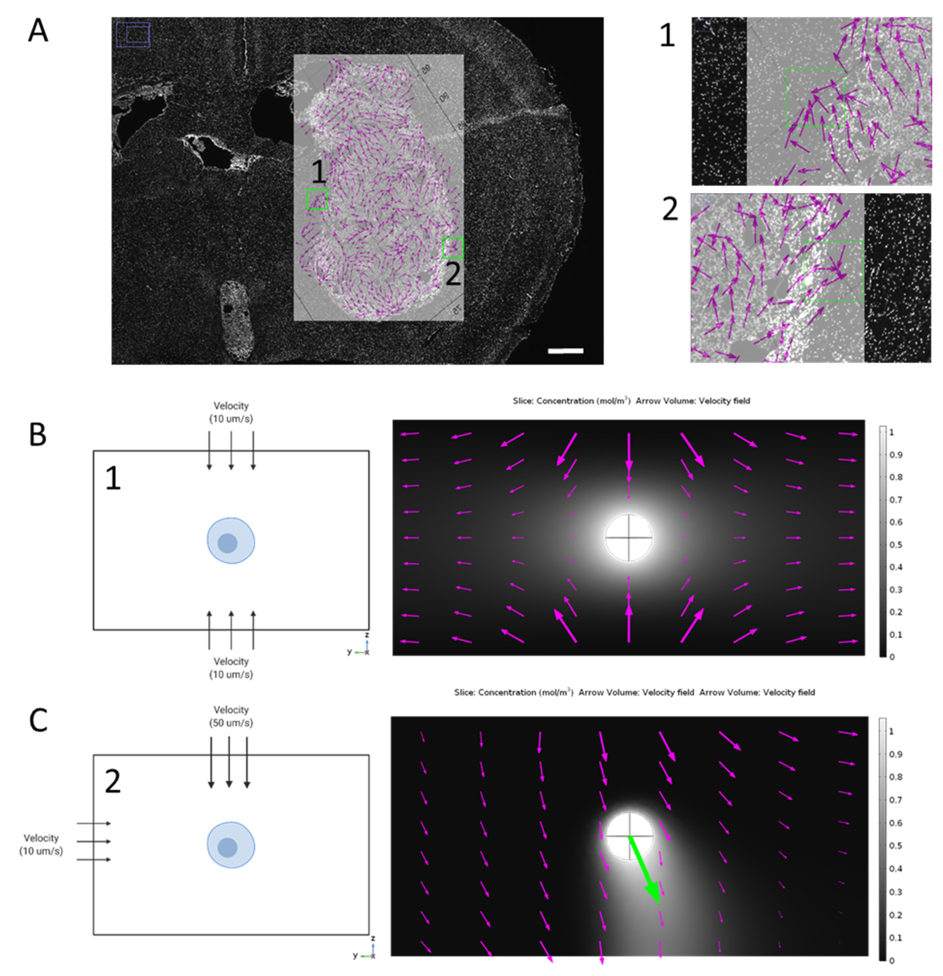
3.2. Directionality of Flow Alters Gradient

Magnitude of interstitial fluid velocity corresponded with increasing concentration gradients across the cell. However, in vivo, we see not only a range of interstitial flow velocity magnitudes, but also direction of the vectors. For example, in mice, we have used dynamic contrast enhanced MRI and mass transport analysis to map interstitial fluid flow velocities across tumors and interstitial space in the brain (Figure 2A). As the tumor progresses, fluid flow becomes heterogeneous especially around the tumor border where invading cells are subjected to its effects. These flow patterns calculated from MRI can be overlaid on histological sections to examine cellular invasion within the brain tissue beyond the tumor border. The resolution of the velocity vector field is 104.2 μm/pixel. We identified and modeled two individual flow patterns (Figure 2(A1,A2)): one where the flow vectors came from opposite sides of the cell and one where the flow was split into an x- and y-component with higher flow in the y-direction (Figure 2B,C). Introducing flow direction from either side of the cell lead to an even distribution of bound CXCL12, with no chemokine gradient formation. Interestingly, while no gradient developed, we did see an induced surface pressure across the cell which might have implications in other cell migration mechanics. When fluid is induced in multiple directions, the formation of the gradient follows the resultant of the flow direction (Figure 2C). We have observed areas of higher invasion in regions of outward fluid flow from the tumor bulk [18], so the development of the gradient in the direction of flow seems to support the idea of autologous chemotaxis. We have also modeled different flow arrangements and have seen this same effect of multidirectional flow skewing the gradient toward the resultant flow direction (Supplemental Figure S5).

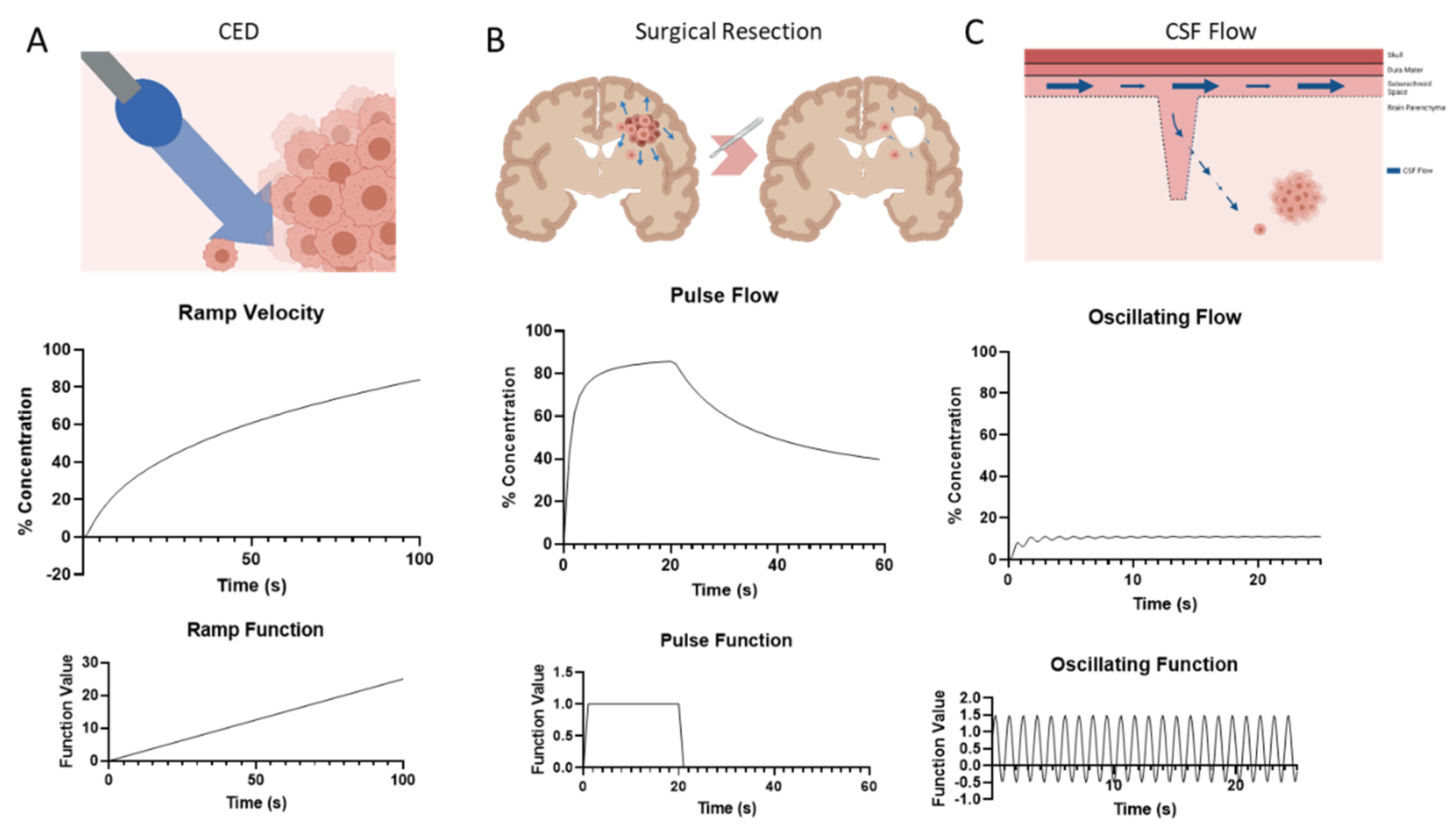
3.3. Temporal Fluctuations in Velocity Yield Variable Gradients

After exploring some of the effects of IFF velocity magnitude and direction, we wanted to understand the time-sensitive effects on gradient formation. Transient solutions were first solved at different time scales in order to investigate the rate at which the gradient formation could actually be observed. Time scales at minutes, seconds, and centiseconds were computed. As shown in Supplemental Figure S6, the gradient can be observed to develop on the centisecond time scale. This seems to be within ranges that have been observed for ligand binding [43]. We next wanted to test the effect that varying flow magnitudes has on the developing cell gradient. We settled on three different conditions that would be physiologically relevant to brain cancer: convection enhanced delivery (CED), surgical resection, and pulsatile flow from cerebrospinal fluid (CSF). Convection enhanced delivery is a treatment method that allows for the bypassing of the blood–brain barrier to deliver therapeutics via catheter directly to the area of the tumor. This method introduces a volume of fluid, which actually increases the interstitial fluid flow throughout the parenchyma. This was modeled as a ramp function with increasing IFF velocity over a short period (Figure 3A) which corresponds to an increasing % concentration that looks almost logarithmic in nature. This is unsurprising based on the results from Figure 1, but we can see that at some point, the gradient starts to drop off as it approaches a potential maximum threshold around 80%. Surgical resection causes a large drop in pressure based on experimental results [44] which we modeled here as a step function in the IFF velocity (Figure 3B). The initial step up shows IFF increase due to tumorigenesis with a steep drop off when resection happens. We see the corresponding rapid increase in bound CXCL12 gradient as the velocity increases, but then almost half a reduction in % concentration as the velocity returns to a more normal value (which would be associated with the resection). Interestingly, the % concentration does not return to normal but instead retains an increased value from baseline. During normal function, the brain has oscillatory flow due to CSF within the subarachnoid and ventricular spaces. We modeled this with a sinusoidal functional based on [41]. With the oscillating function that is net positive, the gradient initially mimics this sinusoidal pattern but quickly converges to a gradient that averages ~13%.

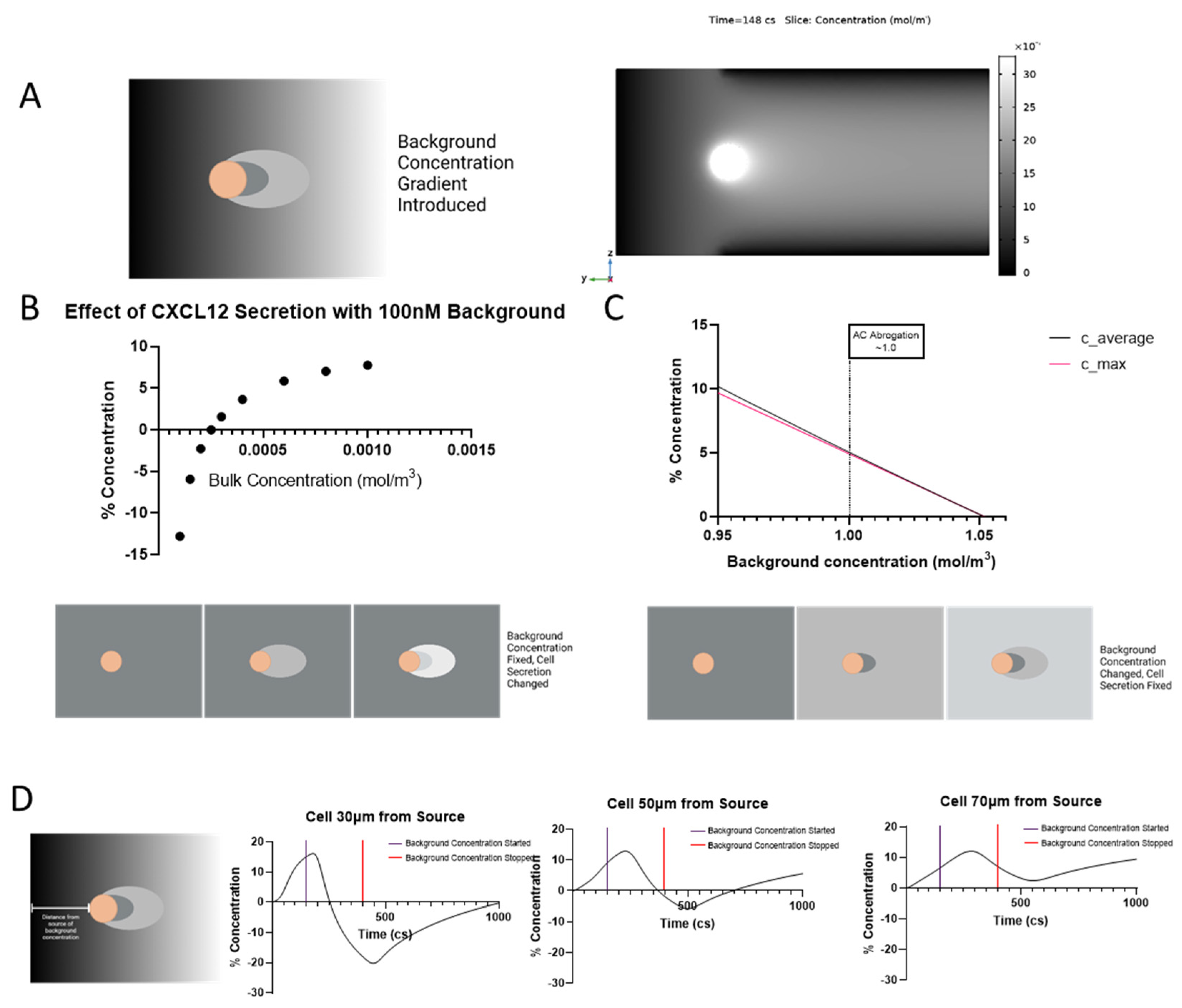
3.4. Background Concentration Can Negate Bound CXCL12 Gradient

As the single tumor cell is not the only contributor to CXCL12 gradients, it is useful to look at how background concentration can affect the development of the autologous gradient. After letting the cell establish its own gradient, we introduce CXCL12 to the background at 150 cs (Figure 4A). The abrogation of the pericellular gradient can be seen over time as the background concentration completely overtakes any gradient development. This abrogation depends on a number of factors such as the bulk concentration of CXCL12 being released by the cell (Figure 4B), the background concentration of CXCL12 that the cell is surrounded by (Figure 4C), and the distance the cell is from the source of the concentration (Figure 4D). If the background CXCL12 is kept constant at 100 nM and the amount of CXCL12 the cell secretes is changed, there is a tipping point where the pericellular gradient starts to form-after 250 nM CXCL12 bulk concentration-after which it reaches a plateau (Figure 4B). If the reverse scenario is explored (constant cell secretion with changing background CXCL12), the pericellular gradient formation is abrogated around 1 mol/m³ (Figure 4C). The position of the cell is also important where background concentration is concerned. As the cell is modeled farther from the source of the background concentration, the pericellular gradient becomes less disrupted to the point that at 70 µm from the source the autologous gradient is still observed for the length of time that the background concentration is applied (Figure 4D). If the cell is closer than 70 μm the background concentration completely abrogates pericellular gradient formation and actually causes a higher concentration of bound CXCL12 to develop upstream of the cell. If the background concentration is removed, the cell reaches a new set point of gradient formation which is notably lower than the starting % concentration the closer the cell is to the source.

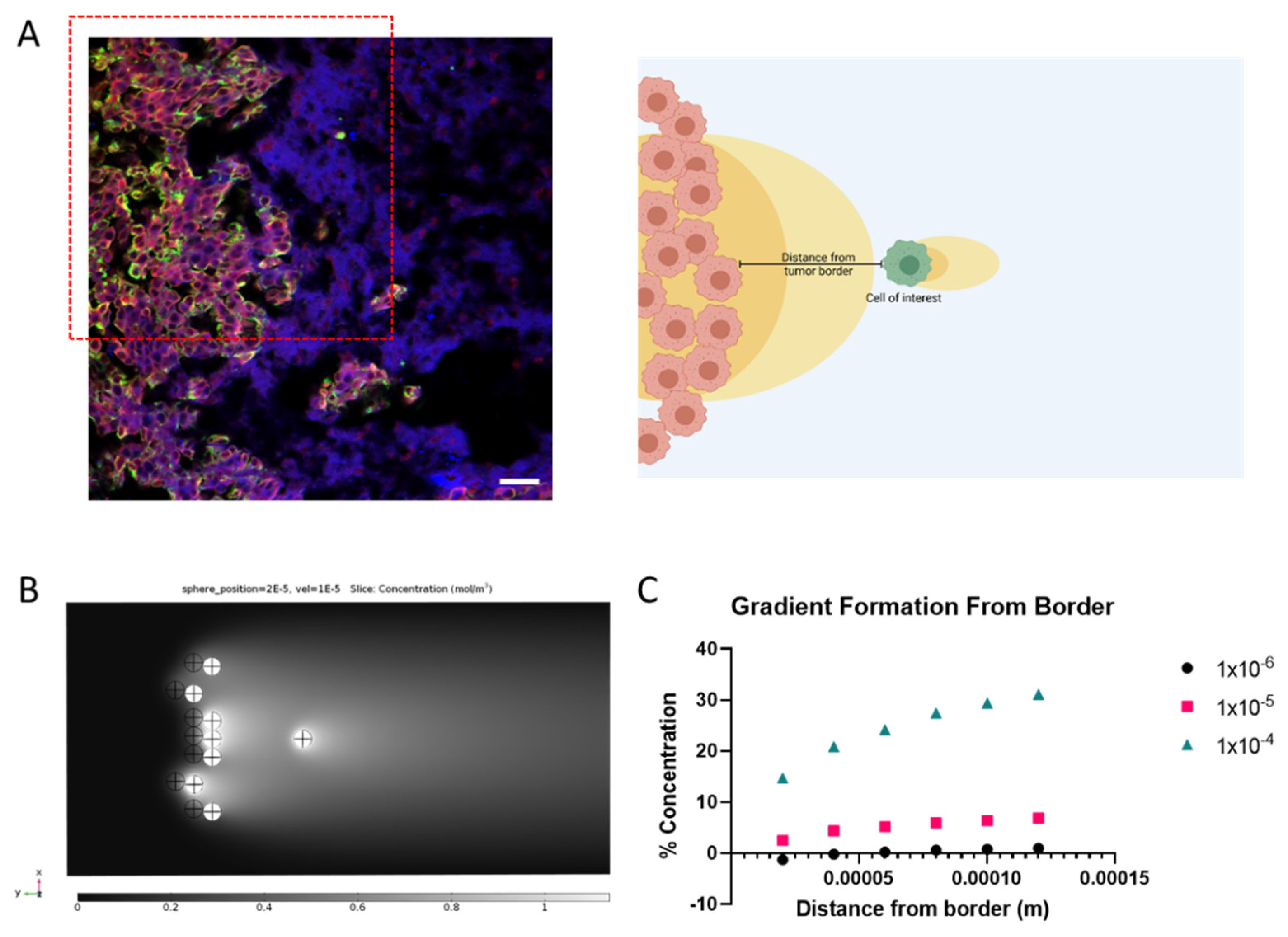
3.5. The Invading Cell Needs to Be a Certain Distance from Tumor Border for Gradient to Develop

Looking into a more physiologically relevant parallel, cells that invade past the tumor border are subjected to varying CXCL12 levels based on the cells at the tumor border that may also secrete CXCL12 as shown in histological samples (Figure 5A). By creating an approximate model with multiple cells on one side of the invading cell and applying CXCL12 secretion to a percentage of those cells, we can model the % concentration that an invading cell would have (Figure 5B,C). As the cell gets farther from the tumor border, the % concentration of bound CXCL12 around the cell increases. In other words, the pericellular gradient can develop without the interference of background CXCL12 secreted by the tumor border in areas where flow is outward. This is further impacted by the magnitude of fluid flow that the cell is under. At higher fluid velocities, the cell is actually able to develop a bound CXCL12 gradient closer to the tumor border. At the lower velocities, the cell cannot overcome the background CXCL12 even at 120 μm away from the border.

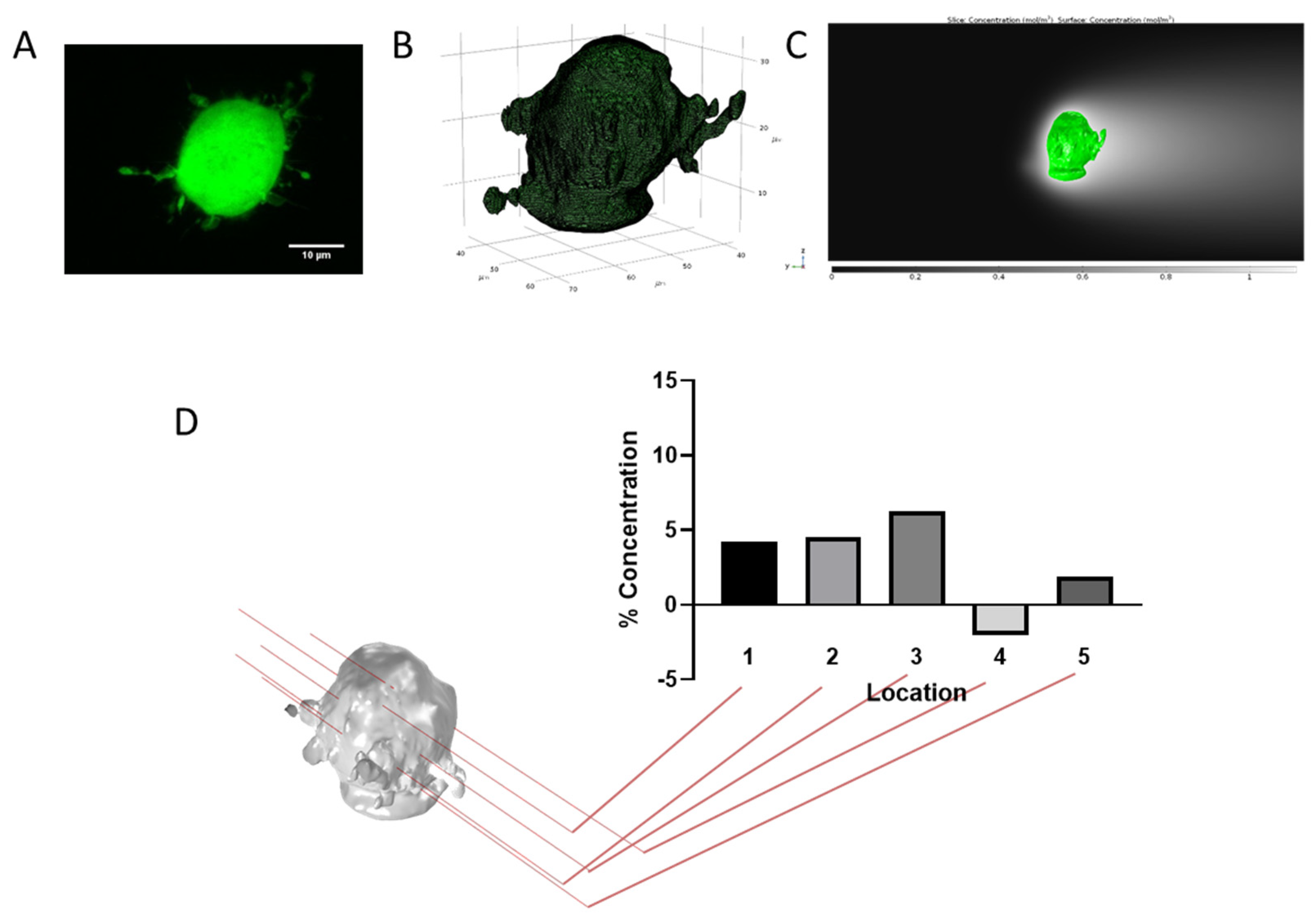
3.6. Cell Type and Morphology Affects Gradient Formation

Up to this point, we have not utilized the full capability of the 3D model as we have concentrated on a readily understandable 2D outcome, % concentration. However, we can probe more complex parameters such as cell size and morphology. As shown in Supplemental Figure S7, cell shape and orientation has a large impact on gradient formation. As the cell increases in diameter, % concentration actually decreases. If we then imagine the cell as an ellipsoid, such as might be seen in a mesenchymal state, we can look into how orientation plays a role in gradient formation. We performed a rotational parametric sweep which shows % concentration is greatest along the long axis of the ellipsoid or when the cell is oriented in the direction of flow (Supplemental Figure S7). When introducing more complex geometry such as that of actual cells, gradient formation becomes heterogeneous and dependent on topography of the cell (Figure 6). In order to accomplish this, we imaged different glioma cells that were within a 3D hydrogel (collagen and hyaluronic acid mixture) at 60× (Figure S7A). The images were then rendered in 3D using a combination of ImageJ and meshing software (refer to the supplemental materials for a detailed description) and imported into the COMSOL model (Figure S7B,C). The overall gradient stays largely the same at the pericellular level but the surface concentration that the cell sees is much more variable (Figure S7D). This topographical heterogeneity is highly dependent on individual cell morphology which complicates matters when trying to understand gradient formation. It may well be that the overall concentration profile is more important than discrete locations on the cell, but this should not be dismissed out of hand.

4. Discussion

In this model, the circumstances leading to and causing autologous gradient formation are investigated to better understand physiologically relevant circumstances with the potential to drive glioma invasion. These glioma cells are introduced to a variety of forces and tissue properties which are heterogeneous by nature. Modulation of individual parameters of the surrounding environment revealed that velocity magnitudes seem to have the highest impact on CXCL12 gradient formation. This may be unsurprising as one would expect higher flow rates to carry chemokines farther and there have been other published models which observe the same for similar chemokines and pathological states [34,35], but it is also complicated by the binding kinetics and tissue properties that are inherent to the system. This does further strengthen the idea, though, that increased interstitial flow magnitudes like those seen in brain cancer can lead to autologous chemotaxis, adding to the invasive potential of tumor cells. The reaction kinetic coefficients were also investigated in order to get an idea of the effect that they have on the model, especially because there is a lack of experimental measurements of these values in the literature. While these should theoretically not change substantially (and not to the extent that we have manipulated in the model), it is worth looking at their impact. From the model results, the % concentration changes from −9 to 25%. This shows a high sensitivity in our model and one that should be further reanalyzed as more data is collected on the binding rates and reaction kinetics of chemokines and their various binding sites. Lastly, the diffusion coefficient is the other variable that the model is sensitive to, with changes to % concentration of −2 to 21%. These changes could be driven by the ECM remodeling that occurs during tumor development, reducing diffusion, but also, we have a hint here of how gradients might form by smaller molecules with higher diffusion coefficients.

We have observed heterogeneous flow magnitude and direction in and around tumors [10]. In patients and in preclinical models, the directionality of IFF is tied to the location of the tumor, surrounding tissue features, and other, as yet unknown drivers. Though the flow-field measured by MRI as depicted in Figure 2 may appear to have multiple directions of flows, ultimately, a cell feels one direction at its scale. Therefore, we see that the gradient around the cell specifically aligns in the direction of the resultant vector of the flow field. Thus, the scale of the flows based on our prior imaging analysis is an oversimplification of the actual flow field which a cell may detect. A cell at the convergence of two flow directions may also sense increased pressures, and we see that here, though we do not account for any deformations that may occur to these cells as a result of their viscoelastic properties as have been seen by others [45]. It has also been shown that fluid flow can fluctuate based on changes in respiration, heart rate, circadian rhythm, and body position (supine vs. sitting) [46,47,48]. These flows happen at different time scales and rates, and are made even more complex when considering pathologic states such as cancer.

Chemokines are released throughout tissue from different cell types within the microenvironment which could impact gradient formation depending on the location of the tumor cell. Specifically, in brain cancer, endothelial cells, immune cells, and astrocytes, in addition to tumor cells, are known producers of CXCL12 [49]. Importantly, CXCL12 also increases after treatment of glioma, specifically after radiation treatment [17,50]. When the background concentration is high enough, the gradient forms in the opposite direction (upstream of the cell instead of downstream), denoted by a negative % concentration value. This finding coincides with our data representing the tumor border. Interestingly, a paradox of the chemotaxis in tumors is that the tumor itself is a reservoir of chemokines such as CXCL12, yet tumor cells still invade away from the bulk. We can see this trend where the gradient is abrogated when the cell is close to the border and begins to form downstream of the cell at a specific distance from the border. The flow magnitude in the local environment also impacts this greatly, with increased velocity causing gradient formation to happen even when the cell is close to the tumor border. In the context of glioma, this is very interesting as it may suggest several things. The first is that invading cells in areas of low flow magnitude must be using multiple modalities by which to move when first invading from the tumor border as the autologous gradient would not have developed in most cases. It is only once the cells reach a certain distance that autologous chemotaxis might be taking place to cause directional tumor cell migration. The other is that under higher flow magnitudes, cells could possibly undergo autologous chemotaxis even when near the tumor border as a way to invade into surrounding tissue. This seems more likely for flow magnitudes between 10 and 100 µm/s which have been observed in human gliomas [42], though not representative of implanted murine models [10].

Most models of gradient formation have modeled idealized rounded cells of similar size, though as with the forces applied to cells, these shapes and sizes are dynamic. Gradient formation was enhanced for smaller cells or cells elongated parallel to the flow direction. This may mean that some cells, or cell states, might be predisposed to autologous chemotaxis-effected movement. The mesenchymal molecular subtype of glioblastoma is marked by increased invasion [51] and may be more likely to display an elongated phenotype. It has been documented that a single tumor can have multiple molecular subtypes [52] and as we have seen heterogeneity in IFF patterns, these factors may combine in intricate ways to modulate regional invasion. Further work, both laboratory and computational, is necessitated to increase the complexity of our simple analyses here. In line with these complexities, the morphology of a single cell is variable as seen in our 3D renderings, and with it so are the arising gradients. Looking at the pericellular gradient as a whole around a cell, the complicated micron-level gradients that form around single parts of the cell disappear. How a cell detects and responds to these micro-gradients is unknown, and would require more advanced experimental systems such as those described in the microfluidics literature [53].

In order to understand what the physiological relevance is of the gradients we have found here, in vitro studies will need to be carried out that vary the concentration of CXCL12 across CXCR4 positive cells. Others have found robust responses to self-generated gradients and thus we suspect these types of responses have potential here [54]. We have not examined the multiple isoforms of CXCL12 nor taken into account other factors of CXCL12 biology which may impact gradient formation and ultimately the cellular consequences of those gradients [37]. The interactions of CXCL12 in our model are simplified and do not account for cellular binding, uptake, recycling, or dimerization that may occur to elicit the downstream cellular signaling involved in mediating glioma invasion [31,37]. The interaction between the CXCL12 gradient modeled here and its receptors CXCR4 and ACKR3 could be probed in future models and expanded to other isoforms [55]. Additionally, we were only concerned with modeling the ECM-bound CXCL12 through HS which does not account for the host of ways in which a cell or the ECM may engage with CXCL12. Introducing other effects on this interaction such as soluble GAGs [56,57], and protease interactions and potential inactivation [31] will help to strengthen this model in future by providing more robust conclusions on how the established gradient might effect the modelled cells. Overall, this model offers an attempt to examine the effects of observed physiological phenomenon in glioma to examine their effects on the generation of CXCL12 gradients. We hope to move forward by not only incorporating the downstream effects of the gradient as cells interact with it, but also to combine our individual manipulations to better understand which governing forces may be driving IFF-mediated invasion heterogeneously into surrounding parenchyma and offer insight into the benefits of targeting this pathway.

5. Conclusions

In conclusion, we have explored the impact of physiological flows and parameters on the formation of autologous gradients around tumor cells. We see that in every case, gradients can form, however, these are often reduced as more tissue-level relevance is added. Not only is the nature of the flow important but also the extracellular context including background gradients and other cells, as would be present at the tumor border. Further, the cell itself, when modeled based on an actual cell which is non-spherical in shape, develops differential gradients depending upon the 2-dimensional cross-section which is examined. These explorations tell us that the formation of autologous gradients in vivo is much more complex than what has been modeled before and what has been replicated in vitro, though further experimental and more advanced modeling work will create a more robust understanding of the interactions of CXCL12 gradients with the cell itself to elicit invasion.

References

1. Barnes, J.M.; Przybyla, L.; Weaver, V.M. Tissue Mechanics Regulate Brain Development, Homeostasis and Disease. J. Cell Sci. 2017, 130, 71–82. [Google Scholar] [CrossRef] [PubMed] [Green Version]
2. Orr, A.W.; Helmke, B.P.; Blackman, B.R.; Schwartz, M.A. Mechanisms of Mechanotransduction. Dev. Cell 2006, 10, 11–20. [Google Scholar] [CrossRef] [PubMed] [Green Version]
3. Polacheck, W.J.; German, A.E.; Mammoto, A.; Ingber, D.E.; Kamm, R.D. Mechanotransduction of Fluid Stresses Governs 3D Cell Migration. Proc. Natl. Acad. Sci. USA 2014, 111, 2447–2452. [Google Scholar] [CrossRef] [PubMed] [Green Version]
4. Miller, R.J.; Rostene, W.; Apartis, E.; Banisadr, G.; Biber, K.; Milligan, E.D.; White, F.A.; Zhang, J. Chemokine Action in the Nervous System. J. Neurosci. 2008, 28, 11792–11795. [Google Scholar] [CrossRef]
5. Wang, J.; Knaut, H. Chemokine Signaling in Development and Disease. Development 2014, 141, 4199–4205. [Google Scholar] [CrossRef] [Green Version]
6. Moore, J.E.; Brook, B.S.; Nibbs, R.J.B. Chemokine Transport Dynamics and Emerging Recognition of Their Role in Immune Function. Curr. Opin. Biomed. Eng. 2018, 5, 90–95. [Google Scholar] [CrossRef] [PubMed]
7. Munson, J.M.; Shieh, A.C. Interstitial Fluid Flow in Cancer: Implications for Disease Progression and Treatment. Cancer Manag. Res. 2014, 6, 317–318. [Google Scholar] [CrossRef] [Green Version]
8. Wagner, M.; Wiig, H. Tumor Interstitial Fluid Formation, Characterization, and Clinical Implications. Front. Oncol. 2015, 5, 115. [Google Scholar] [CrossRef] [Green Version]
9. Müller, A.; Homey, B.; Soto, H.; Ge, N.; Catron, D.; Buchanan, M.E.; McClanahan, T.; Murphy, E.; Yuan, W.; Wagner, S.N.; et al. Involvement of Chemokine Receptors in Breast Cancer Metastasis. Nature 2001, 410, 50–56. [Google Scholar] [CrossRef]
10. Kingsmore, K.M.; Vaccari, A.; Abler, D.; Cui, S.X.; Epstein, F.H.; Rockne, R.C.; Acton, S.T.; Munson, J.M. MRI Analysis to Map Interstitial Flow in the Brain Tumor Microenvironment. APL Bioeng. 2018, 2, 031905. [Google Scholar] [CrossRef]
11. Shetty, A.K.; Zanirati, G. The Interstitial System of the Brain in Health and Disease. Aging Dis. 2020, 11, 200–211. [Google Scholar] [CrossRef] [PubMed] [Green Version]
12. Iliff, J.J.; Wang, M.; Liao, Y.; Plogg, B.A.; Peng, W.; Gundersen, G.A.; Benveniste, H.; Vates, G.E.; Deane, R.; Goldman, S.A.; et al. A Paravascular Pathway Facilitates CSF Flow Through the Brain Parenchyma and the Clearance of Interstitial Solutes, Including Amyloid b. Sci. Transl. Med. 2012, 4, 147ra111. [Google Scholar] [CrossRef] [Green Version]
13. Weller, R.O. Pathology of Cerebrospinal Fluid and Interstitial Fluid of the CNS: Significance for Alzheimer Disease, Prion Disorders and Multiple Sclerosis. J. Neuropathol. Exp. Neurol. 1998, 57, 885–894. [Google Scholar] [CrossRef] [Green Version]
14. Kingsmore, K.M.; Logsdon, D.K.; Floyd, D.H.; Peirce, S.M.; Purow, B.W.; Munson, J.M. Interstitial Flow Differentially Increases Patient-Derived Glioblastoma Stem Cell Invasion: Via CXCR4, CXCL12, and CD44-Mediated Mechanisms. Integr. Biol. 2016, 8, 1246–1260. [Google Scholar] [CrossRef]
15. Shieh, A.C.; Swartz, M.A. Regulation of Tumor Invasion by Interstitial Fluid Flow. Phys. Biol. 2011, 8, 015012. [Google Scholar] [CrossRef]
16. Boucher, Y.; Salehi, H.; Witwer, B.; Harsh, G.R.; Jain, R.K. Interstitial Fluid Pressure in Intracranial Tumours in Patients and in Rodents. Br. J. Cancer 1997, 75, 829–836. [Google Scholar] [CrossRef] [PubMed]
17. Cornelison, R.C.; Brennan, C.E.; Kingsmore, K.M.; Munson, J.M. Convective Forces Increase CXCR4-Dependent Glioblastoma Cell Invasion in GL261 Murine Model. Sci. Rep. 2018, 8, 17057. [Google Scholar] [CrossRef] [Green Version]
18. Munson, J.M.; Bellamkonda, R.V.; Swartz, M.A. Interstitial Flow in a 3d Microenvironment Increases Glioma Invasion by a Cxcr4-Dependent Mechanism. Cancer Res. 2013, 73, 1536–1546. [Google Scholar] [CrossRef] [PubMed] [Green Version]
19. Balkwill, F. Cancer and the Chemokine Network. Nat. Rev. Cancer 2004, 4, 540–550. [Google Scholar] [CrossRef]
20. Lacalle, R.A.; Blanco, R.; Carmona-Rodríguez, L.; Martín-Leal, A.; Mira, E.; Mañes, S. Chemokine Receptor Signaling and the Hallmarks of Cancer. Int. Rev. Cell Mol. Biol. 2017, 331, 181–244. [Google Scholar] [CrossRef]
21. Shields, J.D.; Randolph, G.J.; Fleury, M.E.; Yong, C.; Swartz, M.A.; Tomei, A.A. Autologous Chemotaxis as a Mechanism of Tumor Cell Homing to Lymphatics via Interstitial Flow and Autocrine CCR7 Signaling. Cancer Cell 2007, 11, 526–538. [Google Scholar] [CrossRef] [PubMed] [Green Version]
22. Loberg, R.D.; Day, L.S.L.; Harwood, J.; Ying, C.; St. John, L.N.; Giles, R.; Neeley, C.K.; Pienta, K.J. CCL2 Is a Potent Regulator of Prostate Cancer Cell Migration and Proliferation. Neoplasia 2006, 8, 578–586. [Google Scholar] [CrossRef] [Green Version]
23. Laguri, C.; Arenzana-Seisdedos, F.; Lortat-Jacob, H. Relationships between Glycosaminoglycan and Receptor Binding Sites in Chemokines-the CXCL12 Example. Carbohydr. Res. 2008, 343, 2018–2023. [Google Scholar] [CrossRef] [PubMed]
24. Netelenbos, T.; Zuijderduijn, S.; van den Born, J.; Kessler, F.; Zweegman, S.; Huijgens, P.C.; Dräger, A.M. Proteoglycans Guide SDF-1-induced Migration of Hematopoietic Progenitor cells. J. Leukoc. Biol. 2002, 72, 353–362. [Google Scholar]
25. Barinov, A.; Luo, L.; Gasse, P.; Meas-Yedid, V.; Donnadieu, E.; Arenzana-Seisdedos, F.; Vieira, P. Essential Role of Immobilized Chemokine CXCL12 in the Regulation of the Humoral Immune Response. Proc. Natl. Acad. Sci. USA 2017, 114, 2319–2324. [Google Scholar] [CrossRef] [Green Version]
26. Logun, M.T.; Bisel, N.S.; Tanasse, E.A.; Zhao, W.; Gunasekera, B.; Mao, L.; Karumbaiah, L. Glioma Cell Invasion Is Significantly Enhanced in Composite Hydrogel Matrices Composed of Chondroitin 4- and 4,6-Sulfated Glycosaminoglycans. J. Mater. Chem. B 2016, 4, 6052–6064. [Google Scholar] [CrossRef] [Green Version]
27. Thakar, D.; Dalonneau, F.; Migliorini, E.; Lortat-Jacob, H.; Boturyn, D.; Albiges-Rizo, C.; Coche-Guerente, L.; Picart, C.; Richter, R.P. Binding of the Chemokine CXCL12α to Its Natural Extracellular Matrix Ligand Heparan Sulfate Enables Myoblast Adhesion and Facilitates Cell Motility. Biomaterials 2017, 123, 24–38. [Google Scholar] [CrossRef]
28. Levicar, N.; Nutall, R.K.; Lah, T.T. Proteases in Brain Tumour Progression. Acta Neurochir. 2003, 145, 825–838. [Google Scholar] [CrossRef] [PubMed]
29. Rao, J.S. Molecular Mechanisms of Glioma Invasiveness: The Role of Proteases. Nat. Rev. Cancer 2003, 3, 489–501. [Google Scholar] [CrossRef]
30. Sadir, R.; Imberty, A.; Baleux, F.; Lortat-Jacob, H. Heparan Sulfate/Heparin Oligosaccharides Protect Stromal Cell-Derived Factor-1 (SDF-1)/CXCL12 against Proteolysis Induced by CD26/Dipeptidyl Peptidase IV. J. Biol. Chem. 2004, 279, 43854–43860. [Google Scholar] [CrossRef] [Green Version]
31. Janssens, R.; Struyf, S.; Proost, P. The Unique Structural and Functional Features of CXCL12. Cell. Mol. Immunol. 2018, 15, 299–311. [Google Scholar] [CrossRef]
32. McQuibban, G.A.; Butler, G.S.; Gong, J.H.; Bendall, L.; Power, C.; Clark-Lewis, I.; Overall, C.M. Matrix Metalloproteinase Activity Inactivates the CXC Chemokine Stromal Cell-Derived Factor-1. J. Biol. Chem. 2001, 276, 43503–43508. [Google Scholar] [CrossRef] [PubMed] [Green Version]
33. Saw, S.; Weiss, A.; Khokha, R.; Waterhouse, P.D. Metalloproteases: On the Watch in the Hematopoietic Niche. Trends Immunol. 2019, 40, 1053–1070. [Google Scholar] [CrossRef] [Green Version]
34. Fleury, M.E.; Boardman, K.C.; Swartz, M.A. Autologous Morphogen Gradients by Subtle Interstitial Flow and Matrix Interactions. Biophys. J. 2006, 91, 113–121. [Google Scholar] [CrossRef] [PubMed] [Green Version]
35. Waldeland, J.O.; Evje, S. A Multiphase Model for Exploring Tumor Cell Migration Driven by Autologous Chemotaxis. Chem. Eng. Sci. 2018, 191, 268–287. [Google Scholar] [CrossRef]
36. Jafarnejad, M.; Zawieja, D.C.; Brook, B.S.; Nibbs, R.J.B.; Moore, J.E. A Novel Computational Model Predicts Key Regulators of Chemokine Gradient Formation in Lymph Nodes and Site-Specific Roles for CCL19 and ACKR4. J. Immunol. 2017, 199, 2291–2304. [Google Scholar] [CrossRef] [Green Version]
37. Chang, S.L.; Cavnar, S.P.; Takayama, S.; Luker, G.D.; Linderman, J.J. Cell, Isoform, and Environment Factors Shape Gradients and Modulate Chemotaxis. PLoS ONE 2015, 10, e0174189. [Google Scholar] [CrossRef] [Green Version]
38. Fournier, R. Basic Transport. Phenomena in Biomedical Engineering, 3rd ed.; CRC Press: Boca Raton, FL, USA, 2011. [Google Scholar]
39. Lui, A.C.P.; Polis, T.Z.; Cicutti, N.J. Densities of Cerebrospinal Fluid and Spinal Anaesthetic Solutions in Surgical Patients at Body Temperature. Can. J. Anaesth. 1998, 45, 297–303. [Google Scholar] [CrossRef] [Green Version]
40. Bloomfield, I.G.; Johnston, I.H.; Bilston, L.E. Effects of Proteins, Blood Cells and Glucose on the Viscosity of Cerebrospinal Fluid. Pediatr. Neurosurg. 1998, 28, 246–251. [Google Scholar] [CrossRef]
41. Linninger, A.A.; Tsakiris, C.; Zhu, D.C.; Xenos, M.; Roycewicz, P.; Danziger, Z.; Penn, R. Pulsatile Cerebrospinal Fluid Dynamics in the Human Brain. IEEE Trans. Biomed. Eng. 2005, 52, 557–565. [Google Scholar] [CrossRef]
42. Chatterjee, K.; Atay, N.; Abler, D.; Bhargava, S.; Sahoo, P.; Rockne, R.; Munson, J. Utilizing Dynamic Contrast-Enhanced Magnetic Resonance Imaging (DCE-MRI) to Analyze Interstitial Fluid Flow and Transport in Glioblastoma and the Surrounding Parenchyma in Human Patients. Pharmaceutics 2021, 13, 212. [Google Scholar] [CrossRef]
43. Corzo, J.; Santamaria, M. Time, the Forgotten Dimension of Ligand Binding Teaching. Biochem. Mol. Biol. Educ. 2006, 34, 413–416. [Google Scholar] [CrossRef]
44. Gaab, M.R.; Knoblich, O.E.; Fuhrmeister, U.; Pflughaupt, K.W.; Dietrich, K. Comparison of the Effects of Surgical Decompression and Resection of Local Edema in the Therapy of Experimental Brain Trauma: Investigation of ICP, EEG and Cerebral Metabolism in Cats. Pediatr. Neurosurg. 1979, 5, 484–498. [Google Scholar] [CrossRef]
45. Armistead, F.J.; Gala De Pablo, J.; Gadêlha, H.; Peyman, S.A.; Evans, S.D. Cells Under Stress: An Inertial-Shear Microfluidic Determination of Cell Behavior. Biophys. J. 2019, 116, 1127–1135. [Google Scholar] [CrossRef] [Green Version]
46. Nilsson, C.; Stahlberg, F.; Thomsen, C.; Henriksen, O.; Herning, M.; Owman, C. Circadian Variation in Human Cerebrospinal Fluid Production Measured by Magnetic Resonance Imaging. Am. J. Physiol.-Regul. Integr. Comp. Physiol. 2017, 262, R20–R24. [Google Scholar] [CrossRef]
47. Battal, B.; Kocaoglu, M.; Bulakbasi, N.; Husmen, G.; Tuba Sanal, H.; Tayfun, C. Cerebrospinal Fluid Flow Imaging by Using Phase-Contrast MR Technique. Br. J. Radiol. 2011, 84, 758–765. [Google Scholar] [CrossRef] [PubMed] [Green Version]
48. Brinker, T.; Stopa, E.; Morrison, J.; Klinge, P. A New Look at Cerebrospinal Fluid Movement. Fluids Barriers CNS 2014, 11, 10. [Google Scholar] [CrossRef] [Green Version]
49. Li, M.; Ransohoff, R.M. Multiple Roles of Chemokine CXCL12 in the Central Nervous System: A Migration from Immunology to Neurobiology. Prog. Neurobiol. 2008, 84, 116–131. [Google Scholar] [CrossRef] [PubMed] [Green Version]
50. Giordano, F.A.; Link, B.; Glas, M.; Herrlinger, U.; Wenz, F.; Umansky, V.; Brown, J.M.; Herskind, C. Targeting the Post-Irradiation Tumor Microenvironment in Glioblastoma via Inhibition of CXCL12. Cancers 2019, 11, 272. [Google Scholar] [CrossRef] [Green Version]
51. Behnan, J.; Finocchiaro, G.; Hanna, G. The Landscape of the Mesenchymal Signature in Brain Tumours. Brain 2019, 142, 847–866. [Google Scholar] [CrossRef] [PubMed] [Green Version]
52. Sottoriva, A.; Spiteri, I.; Piccirillo, S.G.M.; Touloumis, A.; Collins, V.P.; Marioni, J.C.; Curtis, C.; Watts, C.; Tavaré, S. Intratumor Heterogeneity in Human Glioblastoma Reflects Cancer Evolutionary Dynamics. Proc. Natl. Acad. Sci. USA 2013, 110, 4009–4014. [Google Scholar] [CrossRef] [PubMed] [Green Version]
53. Yamahira, S.; Satoh, T.; Yanagawa, F.; Tamura, M.; Takagi, T.; Nakatani, E.; Kusama, Y.; Sumaru, K.; Sugiura, S.; Kanamori, T. Stepwise Construction of Dynamic Microscale Concentration Gradients around Hydrogel-Encapsulated Cells in a Microfluidic Perfusion Culture Device. R. Soc. Open Sci. 2020, 7, 200027. [Google Scholar] [CrossRef] [PubMed]
54. Tweedy, L.; Insall, R.H. Self-Generated Gradients Yield Exceptionally Robust Steering Cues. Front. Cell Dev. Biol. 2020, 8, 133. [Google Scholar] [CrossRef] [PubMed] [Green Version]
55. Shi, Y.; Riese, D.J.; Shen, J. The Role of the CXCL12/CXCR4/CXCR7 Chemokine Axis in Cancer. Front. Pharmacol. 2020, 11, 1969. [Google Scholar] [CrossRef] [PubMed]
56. Seeger, F.H.; Rasper, T.; Fischer, A.; Muhly-Reinholz, M.; Hergenreider, E.; Leistner, D.M.; Sommer, K.; Manavski, Y.; Henschler, R.; Chavakis, E.; et al. Heparin Disrupts the CXCR4/SDF-1 Axis and Impairs the Functional Capacity of Bone Marrow–Derived Mononuclear Cells Used for Cardiovascular Repair. Circ. Res. 2012, 111, 854–862. [Google Scholar] [CrossRef] [Green Version]
57. Zhou, Z.-H.; Karnaukhova, E.; Rajabi, M.; Reeder, K.; Chen, T.; Dhawan, S.; Kozlowski, S. Oversulfated Chondroitin Sulfate Binds to Chemokines and Inhibits Stromal Cell-Derived Factor-1 Mediated Signaling in Activated T Cells. PLoS ONE 2014, 9, e94402. [Google Scholar] [CrossRef]
Figure 1. Modulation of transport parameters yields expected responses in gradient formation. (A) Representative images of three different diffusion coefficient combinations which create varying bound CXCL12 gradients around the cell. (B) Quantification of % concentration (bound CXCL12) around the cell. (C) Representative images of three combinations of reaction coefficients showing the differential response of gradient formation. (D) Quantification of bound CXCL12 around the cell with varying reaction coefficients. (E) Representative images of gradient formation with increasing velocity. (F) Quantification of % concentration at varying velocities. (G) Schematic of model and % concentration calculation. (H) Regression of relationship between % concentration and velocity, showing positive correlation between the two.
Biophysica 02 00003 g001
Figure 2. Multidirectional flow and its impact on gradient formation around a single cell. (A) MRI analysis of interstitial fluid flow magnitude and direction overlayed on histological sample showing flow heterogeneity and two specific regions of interest (1) and (2). Scale bar 0.5 mm. (B) Schematic of flow directed evenly on the top and bottom of the cell (left) and resulting flow pathways overlayed on top of bound CXCL12 gradient (right) around a single cell (10µm diameter). (C) Schematic of flow directed above and to the left of the cell (left) and resulting flow pathway (magenta arrows) with corresponding resultant of flow direction (green arrow) overlayed on bound CXCL12 gradient (right).
Biophysica 02 00003 g002
Figure 3. Transient solutions of gradient formation around single cells based on physiological time-dependent changes to superficial flow rate. (A) Schematic of CED increasing fluid flow (top) followed by the resulting concentration gradient over time (middle), and the ramp function input into COMSOL (bottom). (B) Schematic of surgical resection impact of fluid flow (top), the resulting concentration gradient over time (middle), and the pulse function input into COMSOL (bottom). (C) Schematic of oscillating CSF flow coming from the Virchow-Robin space into the parenchyma and interacting with tumor cells (top), the resulting concentration gradient over time (middle), and the oscillating function input into COMSOL (bottom).
Biophysica 02 00003 g003
Figure 4. Background concentration reduces the concentration gradient around single cell. (A) Schematic of background concentration around a secreting cell (left) and timelapse video of background concentration added at 150 cs (right). Note that timelapse images are not to the same scale in order to better show background concentration. (B) Modulating cellular secretion rate of CXCL12 while keeping a constant background CXCL12 concentration of 100 nM. (C) Amount of background bound CXCL12 needed to decrease the cellular gradient below 5%. (D) Impact of distance between cell and source of CXCL12 background on gradient formation.
Biophysica 02 00003 g004
Figure 5. Concentration gradients felt by an invading cell beyond the tumor border at varying distance (A) Immunohistochemistry of tumor border and invading cell (green) with CXCR4 (red) and CXCL12 (blue) (left) and schematic representing model parameters of interest (right). Scale bar = 50 µm (B) Representative image of gradient formation of cell with tumor border CXCL12 secretion. (C) Quantification of gradient formation around invading cell depending on distance from tumor border and velocity of IFF.
Biophysica 02 00003 g005
Figure 6. Concentration gradients depend on location along a morphologically accurate tumor cell. (A) Confocal image of GL261. (B) 3D rendering and mesh used in the model. (C) Representative images of cell imports into model and resulting concentration profiles. (D) Quantification of % concentration at different points on the cell.
Biophysica 02 00003 g006