High-Resolution Subsurface Characterization Using Seismic Inversion—Methodology and Examples

Abstract

Subsurface characterization for lithological and fluid properties is important for all aspects of geophysical exploration where estimating a high-resolution elastic property through seismic inversion is vital. Starting with an initial subsurface model, computing synthetic or predicted seismic data, and matching these data with observed seismic data, seismic inversion uses an optimization process to iteratively modify the initial model until the prediction reasonably matches the observation. Routine applications of seismic inversion for subsurface reservoir characterization are currently restricted to amplitude-variation-with-angle inversion, which uses convolution as the basis for forward modeling to compute synthetic seismic data. Although computationally efficient, the inherent convolutional assumption ignores complex wave propagation effects and often fails to estimate subsurface models with sufficient accuracy. Here, we review the current state of the art for seismic inversion, and we discuss a method that uses an analytical wave equation solver for forward modeling and a global method for optimization that can overcome the current limitations of amplitude-variation-with-angle inversion. Using real seismic data, we demonstrate the accuracy of this method. Because this waveform-based method is computationally demanding, we also discuss the current advances of computational technology, including artificial intelligence that can improve its computational efficiency.

1. Introduction

Characterizing the subsurface for lithological and fluid properties such as porosity, permeability, lithology, fluid saturation and pressure, and in situ stress fields is vital for all aspects of fossil fuel-based (oil and gas) energy exploration and production and is routinely used in the oil and gas industry. These properties can be directly measured at well locations. It is, however, necessary to estimate them in between wells, where seismic inversion plays a primary role. Seismic inversion is an optimization method that allows for estimating subsurface elastic Earth properties, such as P- and S-wave velocities ($V_P,V_S$) and density ($\rho$), from observed seismic data. These elastic properties, in combination with rock–physics modeling and inversion, can be mapped onto the lithological and fluid properties in between well locations. Once the elastic Earth properties are estimated from seismic inversion, a variety of rock–physics tools can be used to map them onto the lithological and fluid properties [1]. However, to allow this mapping, accurately estimating the elastic properties through seismic inversion is essential.

Going beyond fossil fuel-based energy, as we move toward the future target of net-zero emissions with a carbon-free grid, the need for accurate seismic inversion is likely to become even more important. To mitigate global warming from fossil fuel usage, for example, there is now a lot of interest in carbon capture and storage (CCS) research. Inverting baseline and time-lapse seismic data and comparing them with one another allows for identifying the time-dependent subsurface movements of injected fluid for all CCS applications. In addition, these inverted data, in conjunction with rock–physics inversion and modeling, reservoir fluid flow, and geomechanical simulations, allow for designing an optimal monitoring, verification, and accounting (MVA) strategy for injected carbon dioxide (CO₂) and other greenhouse gases [2]. To achieve the net-zero target, however, CCS is not sufficient, and enhancing energy production from other alternate resources is crucial. Geothermal energy, especially enhanced geothermal systems (EGSs), is not only an energy resource but also a resource for harnessing energy-critical minerals like lithium [3]. The sustenance of these reservoirs requires routine subsurface characterization [4], where seismic inversion must play a vital role. Energy production from other resources like wind, solar, and hydropower seasonally fluctuates, with periods of energy excesses and deficits. Therefore, without devising means for energy storage, they cannot meet future demands. Producing and storing hydrogen (H₂) underground during excess periods of these alternative forms of energy production and using it for energy production during deficits can meet such demands. This, again, requires subsurface characterization to optimize H₂ storage and production [5,6,7], where the use of seismic inversion is critical [8]. Therefore, seismic inversion is and will continue to remain a vital element in energy technology.

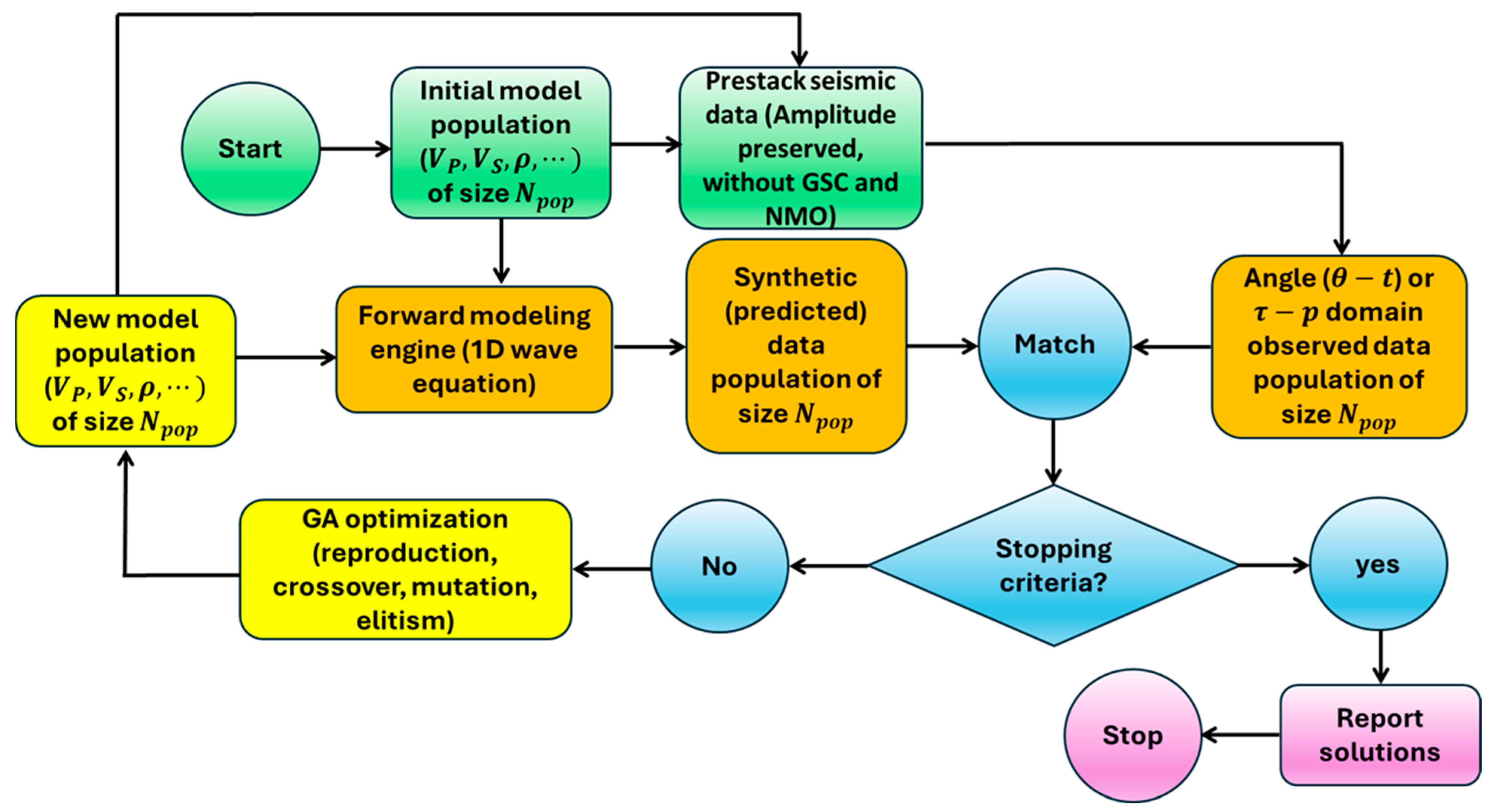
Seismic inversion can be broadly classified into poststack and prestack inversion. Poststack inversion is applied to stacked seismic data. Reflections on stacked seismic data represent normal ($0°$) incident angle reflections, whose amplitudes are sensitive to the acoustic impedance (velocity times density) contrasts across the subsurface layer boundaries. Consequently, we can only estimate the subsurface acoustic impedance through this method. In the past, poststack was the primary seismic inversion tool, not only because computers were not fast enough but also because they did not have sufficient memory. Because of its simplicity and ease of use, this method is still popular, specifically as a reconnaissance tool [9]. With the advances in computing technology, inverting prestack seismic data became feasible for reservoir-related applications, and poststack inversion has now been replaced by prestack inversion. Figure 1 shows the general workflow of these prestack inversion methods, where the input modules are shaded in green; the two main inversion modules, (1) the forward modeling engine used to compute synthetic data and (2) the model performing modifications via optimization, are shaded in orange and yellow, respectively; the iterative process of switching between forward modeling and optimization via matching and eventually entering the output modules is shaded in blue; and the output modules are shaded in purple.

As we can see in Figure 1, the inputs to prestack seismic inversion are (1) the initial model, which we obtain from our geological knowledge and other observations such as well logs, and (2) prestack seismic data (observed data). Restricting to isotropic elastic inversion, the initial model is the model of the P- and S-wave velocities ($V_P,V_S$) and density ($\rho$) as functions of depth or time. We also emphasize that the observed data are the prestack seismic data that are relative amplitude-preserved (RAP). Estimating a subsurface model of $V_P,V_S$, and $\rho$ requires the prestack seismic data to be processed through an RAP processing workflow, which we elaborate further below. Using the initial model, we run the forward modeling engine to compute the synthetic or predicted prestack seismic data. Next, we perform a convergence check by matching the predicted synthetic data with the observed data. If the match is not satisfactory, we use an optimization procedure to modify the model, recompute the synthetic data and match them with observations, and remodify the model. We continue this iterative process until the point where the computed synthetic data satisfactorily match the observations, and then we report solutions and exit via output modules. Based on the general workflow in Figure 1, prestack inversion methods can be classified in two ways: (1) the forward modeling engine used to compute the synthetic data (the box shaded in orange in Figure 1) and (2) the optimization method used to iteratively modify the model (the box shaded in yellow in Figure 1).

Within the broad spectrum of the different forward modeling methods used to compute synthetic seismograms, the current industry practice for prestack seismic inversion is focused on two extreme ends: (1) amplitude-variation-with-angle (AVA) inversion [10,11] and (2) full-waveform inversion (FWI) [12]. In addition, elastic impedance (EI) [13] inversion and extended elastic impedance (EEI) [14] inversion are also popular. EI and EEI are, however, subsets of AVA, and, therefore, we classify them here as AVA inversion. Subsurface characterization demands estimating a high-resolution elastic model from seismic inversion. Although AVA provides this resolution, the forward modeling engine of AVA is convolution-based and thus ignores complex wave effects and often fails to estimate an accurate elastic model [15,16]. FWI, however, uses complete physics by numerically solving the seismic wave equation as the forward modeling engine. However, the computation cost and the curse of high dimensionality limit FWI applications to low resolution, which is suitable for imaging but not for subsurface characterization [17]. In between FWI and AVA, a method that we refer to here as prestack waveform inversion (PWI) was also introduced [18,19,20,21,22,23,24,25,26,27,28]. PWI is a subset of FWI that analytically solves the one-dimensional (1D) wave equation for computing synthetic seismic data. Because of the 1D assumption, PWI is strictly valid for horizontally stratified layers. However, although never explicitly mentioned, all AVA inversion methods are also based on this 1D assumption. To approximately validate this assumption, AVA inversions are typically applied to prestack migrated data. Migration is the process of moving the reflection from all source–receiver pairs to their common image points. For a simple-to-moderate subsurface geology, the common image gathers (CIGs) from prestack migration can be regarded as locally 1D, to which both AVA inversion and PWI can be applied [29].

Besides classifying based on the forward modeling engine, prestack seismic inversion can also be classified based on the optimization method used for iterative model adjustment. In gradient-based or local methods, such as the steepest descent, conjugate gradient, and Gauss–Newton methods, the gradient of the error or misfit function between the observed and synthetic data, also known as the objective, is used as a guide to find a new model for each iteration step, and this continues until the point that the misfit function is less than a certain user-defined tolerance [30,31,32,33,34,35]. In nonlinear or global methods, such as the Markov Chain Monte Carlo (MCMC), simulated annealing (SA), very fast simulated annealing/reannealing (VFSA/VFSR), genetic algorithm (GA), and particle swarm optimization (PSO) methods, models are randomly searched within the model space to find the model or a suite of models that reasonably match observations [36].

Both global and local methods can be combined with the corresponding forward modeling method used to cast inversion in a Bayesian framework. In this framework, we treat the model parameters as random variables. Starting with the prior distributions of each model parameter, such as $V_P,V_S$, and $\rho$, we combine them with the corresponding physics of the forward problem (forward modeling engine) to compute their corresponding posterior probability density functions (PDFs) [37,38,39,40,41,42,43,44,45,46,47]. Casting inversion in a Bayesian framework allows for estimating the PDFs of each model parameter, from which we can not only estimate the maximum likelihood model but also quantify the uncertainties associated with these estimates.

In this paper, we first review the fundamental principles of AVA inversion, its inherent assumptions, and their drawbacks and consequences, and we discuss how using a wave equation-based method in place of a convolution-based method as the forward modeling engine can overcome the drawbacks of AVA. Next, we discuss PWI with genetic algorithm (GA)-based global optimization and detailed aspects of its implementation. Using real seismic data, we then compare PWI with AVA inversion. Finally, we analyze the results, discuss directions for future research on seismic inversion using artificial intelligence, and make concluding remarks.

2. Amplitude-Variation-with-Angle (AVA) Inversion and Its Limitations

The fundamental principle of AVA inversion is convolutional modeling. This convolutional modeling implies that the reflection coefficient, convolved with the seismic wavelet, is an appropriate representation of the seismic data. For simplicity, we use P-wave reflection only where the convolutional modeling assumes that the synthetic seismic data $S_{syn}\left(\theta ,t\right)$ for any given angle of incidence $\theta$ and time sample $t$ are a convolution, given as

$$S_{syn}\left(\theta ,t\right)=w\left(t\right)\ast R_{PP}\left(\theta ,t\right).$$

(1)

In Equation (1), $w\left(t\right)$ is the seismic wavelet, $R_{PP}\left(\theta ,t\right)$ is the P-P reflection coefficient (the ratio between the reflected and incident P-wave amplitudes) as a function of $\theta$ and $t$, and the symbol $\ast$ represents convolution. Restricting to an isotropic elastic case, $R_{PP}$ is a function of $V_P,V_S$, and $\rho$ [48]. Thus, starting with an initial model of $V_P,V_S$, and $\rho$, AVA inversion computes $S_{syn}\left(\theta ,t\right)$ using Equation (1) for a given set of incidence angles ($\theta$) and matches them with the observed seismic data $S_{obs}\left(\theta ,t\right)$ for the same set of incidence angles. Then, by iteratively modifying $V_P,V_S$, and $\rho$ via optimization until $S_{syn}$ and $S_{obs}$ satisfactorily match, the method obtains an estimate of the subsurface model. By repeating this process for each common midpoint (CMP) location over a three-dimensional (3D) prestack data volume, AVA inversion estimates the subsurface elastic model for the volume. Because computing $R_{PP}\left(\theta ,t\right)$ using either the exact reflection coefficient formula or its linearized approximation [49] is computationally efficient, AVA inversions are cost effective, especially for handling large 3D data volumes.

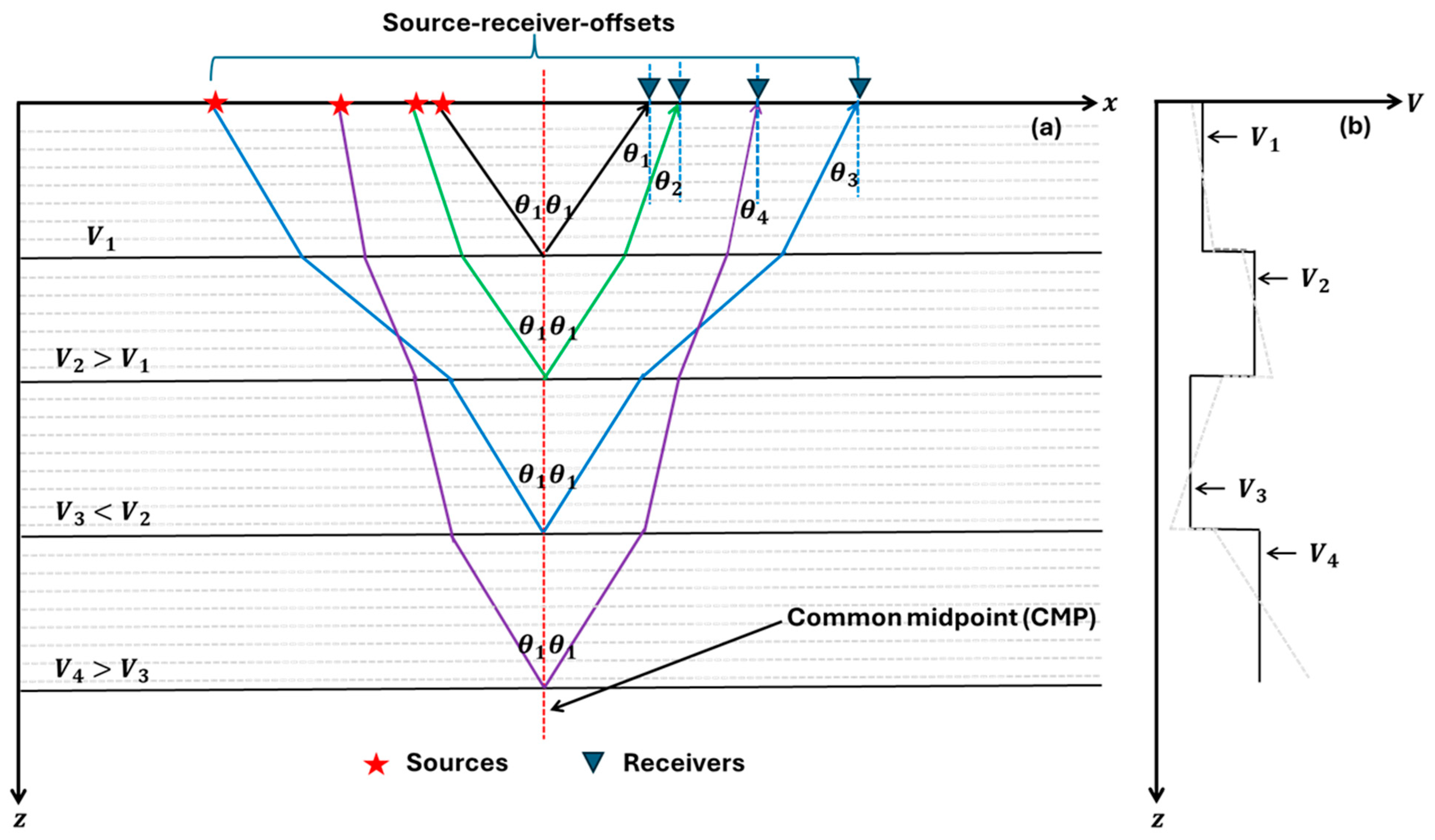
Note that AVA requires the observed seismic data $S_{obs}$ to be in the incidence angle and time domain. Seismic data are, however, acquired in the offset–time ($x-t$) domain, not in the $\theta -t$ domain. So, to apply AVA inversion, it is first necessary to transform $x-t$-domain data into the $\theta -t$ domain. We use Figure 2, Figure 3, Figure 4, Figure 5, Figure 6 and Figure 7 to illustrate $x-t$-to-$\theta -t$ transformation, the problems associated with convolutional modeling, and how we can overcome them using a wave equation instead of a convolution approach for forward modeling.

We start with a simple horizontally stratified four-layer model, underlain by a half space, shown in Figure 2a, with the horizontal (source–receiver offset) and vertical (depth) axes designated by $x$ and $z$, respectively. The four layers with P-wave velocities $V_1,V_2,V_3$, and $V_4$ are indicated by solid black lines. Also, in Figure 2b, we visually illustrate the velocities $V_1,V_2,V_3$, and $V_4$, with velocity $V$ as the horizontal axis and depth as the vertical axis. Please also note that, in Figure 2, we designate the vertical axes as depth $z$. In dealing with seismic data, however, they are measured in the time domain, or, specifically, in the two-way time domain $t$. In the following, we therefore freely switch between depth and time to represent the vertical axis.

Now, consider the source–receiver pairs from a common midpoint (CMP), designated by a red (dashed) vertical line in Figure 2a, which reflect with the same incidence angle ${\theta }_1$ from the four interfaces represented by black, green, blue, and purple ray paths in Figure 2a. It is evident that, to map seismic data from $x-t$ to $\theta -t$, we must draw constant-angle ray paths for the desired range of incidence angles like the one shown in Figure 2a and gather data from different ranges of source–receiver offset values for different times from the $x-t$-domain data. It is also evident that, when velocity increases with depth (time), the source–receiver offsets for a given incidence angle (${\theta }_1$) increase with increasing time, as shown by the reflections from interfaces 1 and 2 (black and green ray paths), where $V_2>V_1$. However, if there is a low-velocity layer in the subsurface followed by a high-velocity layer, the ray paths bend in the opposite direction, causing the source–receiver offsets needed for the same angle ${\theta }_1$ to be lower for higher depths (times) than those needed for lower depths (times). This is shown for the reflection from interfaces 3 and 4. Because $V_3<V_2$, the ray paths in layer 3 bend in the direction opposite to that in layer 2, causing the required source–receiver offset for the incidence angle ${\theta }_1$ for layer 3 reflection to be very high (see the blue ray path). However, because $V_4>V_3$, the ray paths in layer 4 bend like in layer 2, causing the source–receiver offset for the layer 4 reflection for the same incidence angle ${\theta }_1$ to be less than that for the layer 3 reflection (see the purple ray path).

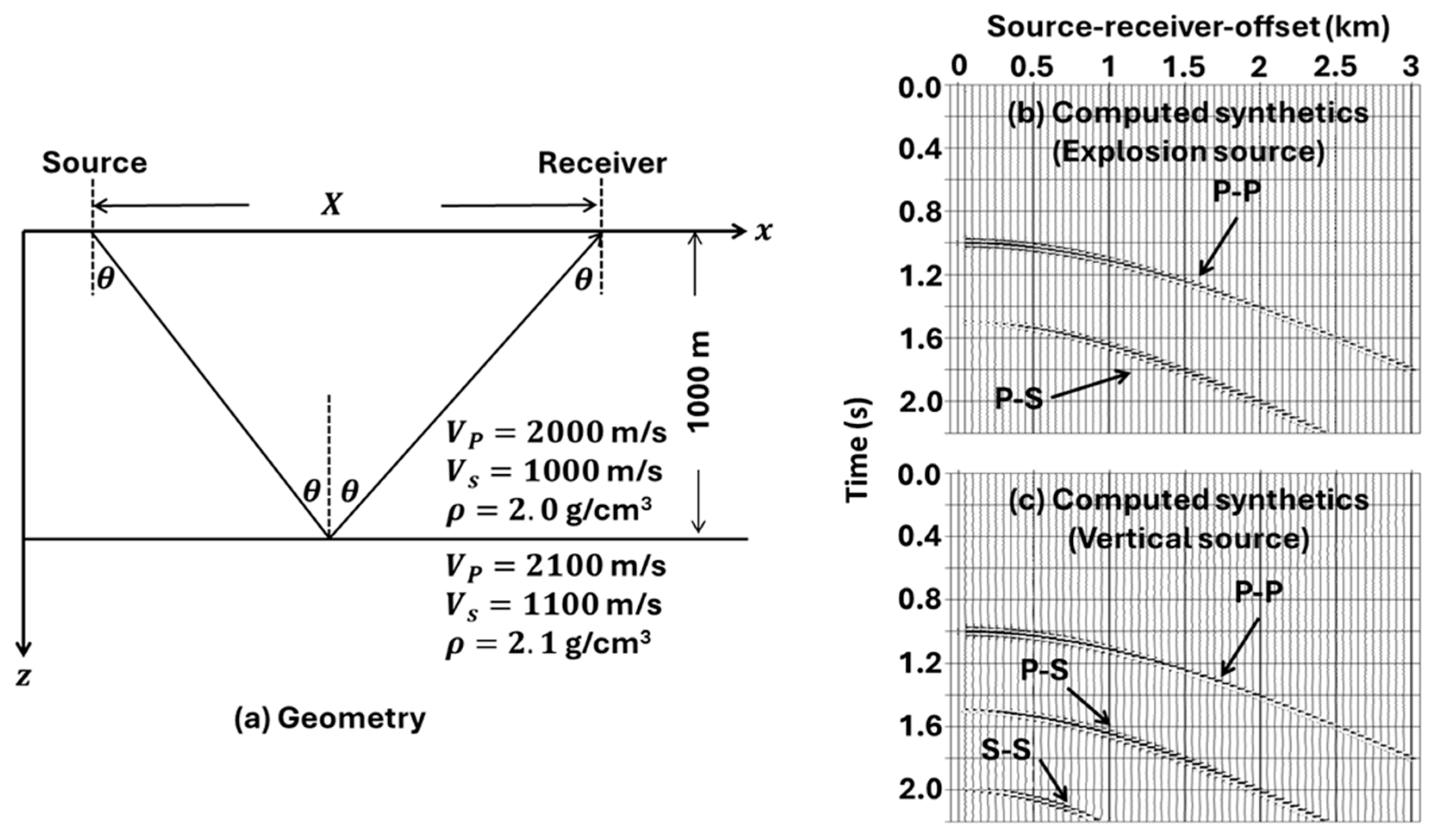
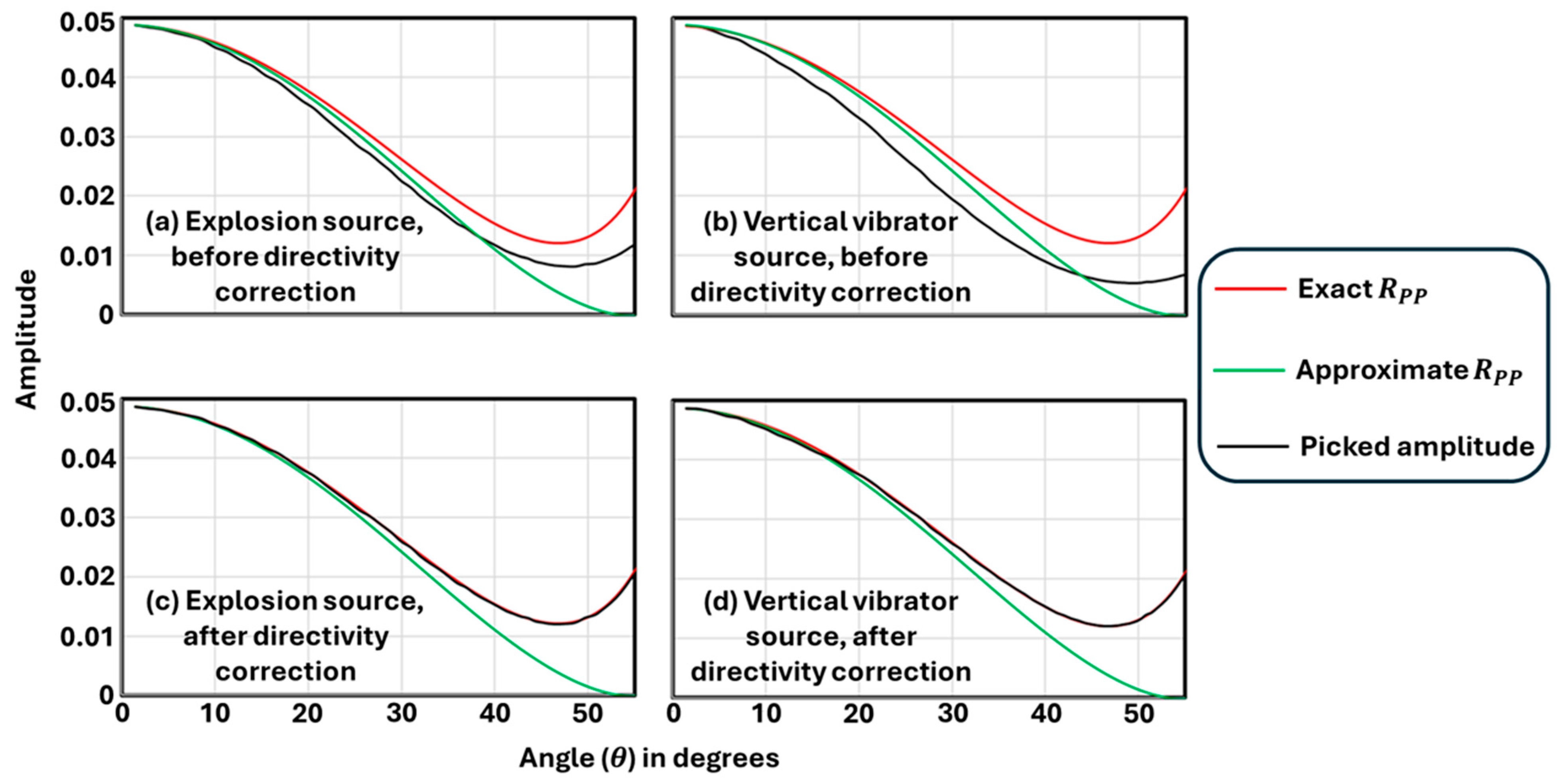
For land seismic data, we typically record the vertical component response (particle velocity or displacement). Recorded amplitudes from this response are not the full reflection coefficients but rather their angle-dependent components. This is the directivity factor, which we must incorporate while computing the convolutional synthetic response. For the layer 1 response, the ray path at the receiver location is at angle ${\theta }_1$ from the vertical component; therefore, only a component of the reflection coefficient should contribute to the vertical component response that the seismic data record. For the reflections for layers 2, 3, and 4, the ray paths are at different angles (${\theta }_2,{\theta }_3,{\theta }_4$), and the vertical component response must be computed by taking the corresponding vertical components of the reflection coefficients for the respective ray path directions. We use Figure 3 and Figure 4 to further explain the directivity factor. Figure 3a shows a layer over a half-space model, in which the P- and S-wave velocities ($V_P,V_S$) and density ($\rho$) of the top layer are 2000 m/s, 1000 m/s, and 2.0 g/cm³, and those for the bottom layer are 2100 m/s, 1100 m/s, and 2.1 g/cm³. We compute the vertical component $x-t$-domain synthetic seismograms for this model using both explosion and vertical vibrator (vertical point force) sources and wave equation-based reflectivity modeling software [50,51,52,53], and the computed results are displayed in Figure 3b,c. Note that the computed synthetics for an explosion source (Figure 3b) contain the primary (P-P) and mode-converted (P-S) reflections. The computed synthetics from the vertical vibrator source (Figure 3c) however contain the S-S reflection in addition to the P-P and P-S reflections. We pick the amplitudes for the P-P reflection from both synthetic data, correct them for the geometrical spreading loss, and compare them with the exact and approximate reflection coefficients given by Aki and Richards (2002) [49] in Figure 4a,b. For each source-to-receiver offset ($x$), their two-way times ($t$), and the layer thickness, we compute the incidence angle ($\theta$), calculate the exact and approximate P-P reflection coefficients ($R_{PP}$), and display the results in these figures, with $\theta$ as the horizontal axis and the picked and corrected amplitude and the computed reflection coefficients as the vertical axis. We must note here that the exact reflection coefficients are functions of the incidence angle $\theta$. The approximate reflection coefficients are, however, functions of the average angle. Therefore, we compute the transmitted angle ${\theta }_T$ for each incidence angle $\theta$ and then use the average angle ${\displaystyle \frac{1}{2}}\left(\theta +{\theta }_T\right)$ to compute the approximate reflection coefficients. Figure 4c,d are the same as Figure 4a,b, except that we correct the picked amplitudes for directivity. For the explosion source, we need correction for the receiver directivity only, and, therefore, we divide the picked amplitudes by $\mathit{cos}\theta$. For the vertical vibrator source, we must account for the directivity from both the source and receiver sides, so we divide the picked amplitudes by ${\mathit{cos}}^2\theta$. Note that, after the directivity correction, the amplitudes of the synthetic seismic data perfectly match the exact $R_{PP}$. The approximate $R_{PP}$, however, closely match the picked amplitudes up to about $\theta =25-30°$, and, beyond that, they significantly differ. In standard seismic processing workflows for $x-t$-to-$\theta -t$ mapping, we usually ignore the issue of directivity, and it is evident from Figure 4 that the effect is significant. It is also important to point out that incorporating this directivity is necessary for land seismic data only, which measure the vertical component response. For marine seismic (streamer) data, where the measured response is pressure, incorporating directivity is not necessary.

Besides the issues discussed in Figure 2, Figure 3 and Figure 4, there is also a loss due to transmission. For reflection from each interface, a part is reflected, and the other part is transmitted. Representing seismic data as convolution (Equation (1)) ignores this amplitude loss from transmission.

Finally, the convolutional assumption means that the recorded seismic data are primary reflections and are not contaminated by multiples, mode conversions (P-S reflection), or other wave effects. This is true when the subsurface layers are widely separated like the four interfaces shown by solid black lines in Figure 2 such that the multiple reflections and mode conversions do not interfere with the primary reflections. In the real world, however, this is unrealistic, and the subsurface consists of many thin layers like the ones indicated by gray dotted lines in Figure 2a, with the corresponding depth varying velocities in Figure 2b. The short-period interbed multiples and mode conversions from these thin layers interfere with the primaries, especially for incidence angles ($\theta$) > 30°. In addition, the rays can also bend and reach a turning point, causing some high-angle reflections not recorded for some time intervals where the subsurface velocity gradients are high. In a modeling study using real well logs, Mallick (2007) [16] demonstrated the severity of these effects. The short-period events from thin layers have moveout almost like primary reflections, and, to the best of our knowledge, there is no data processing technique that can eliminate them.

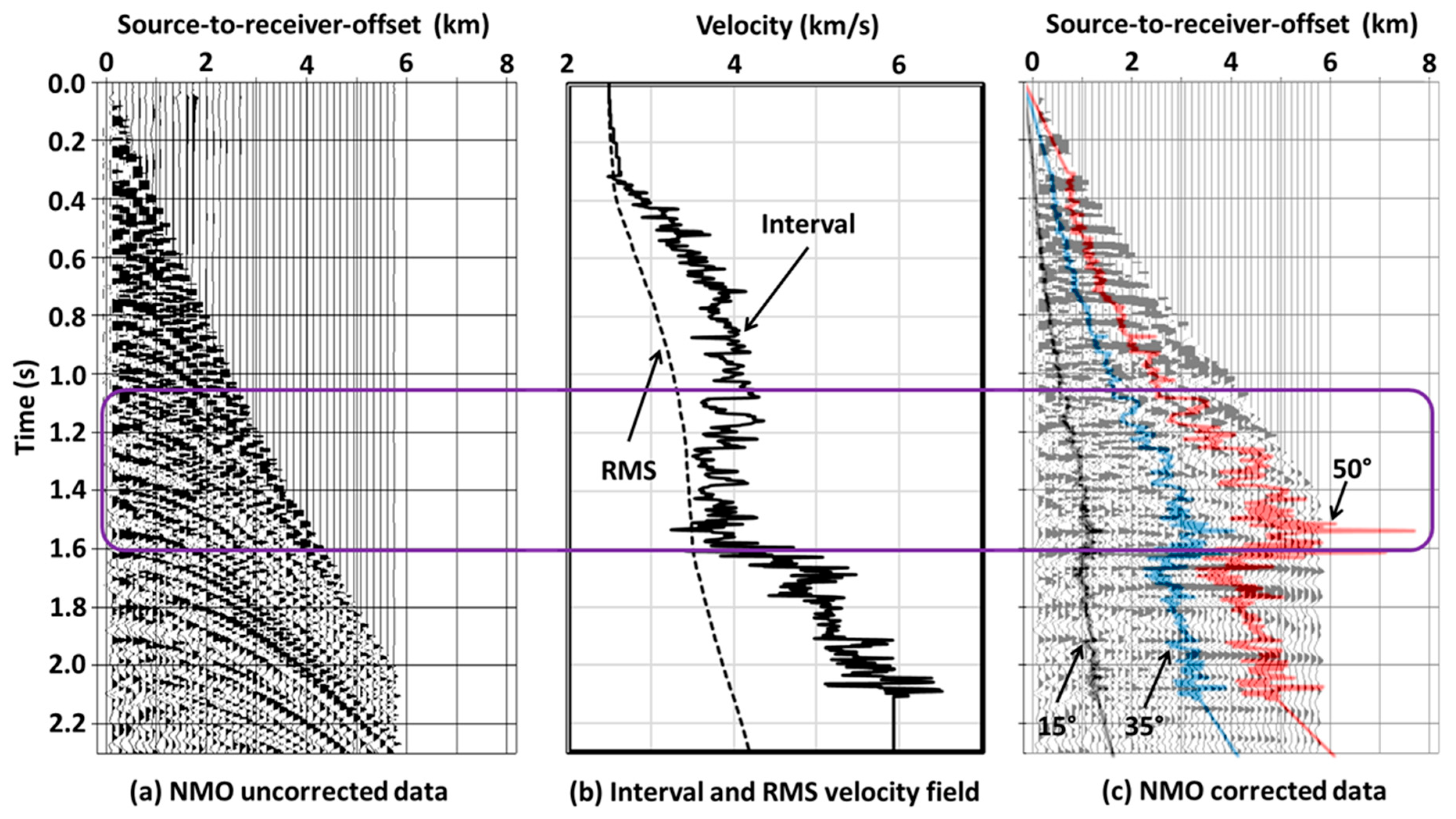
Having demonstrated the offset-to-angle mapping using Figure 2 and the other related issues using Figure 3 and Figure 4, we now use real seismic and well log data to demonstrate how to perform $x-t$-to-$\theta -t$ mapping in practice, which will further emphasize the shortcomings of convolutional modeling and lay the foundations for the appropriateness of using a wave equation method as the basis for the forward modeling engine in Figure 1. Figure 5a shows the real $x-t$-domain data without geometrical spreading compensation (GSC) and normal moveout (NMO) correction. These data are from the Rock Springs Uplift (RSU), Wyoming, USA, which coincides with the location of the RSU#1 well log. The seismic-to-well-tied interval and computed root-mean-square (RMS) P-wave velocities for this RSU #1 well log are shown in Figure 5b. The seismic data in the background of Figure 5c are the GSC- and NMO-corrected data in Figure 5a with the RMS velocity field in Figure 5b, on top of which the constant incidence angle trajectories for the 15$°$, 35$°$, and 50° incidence angles, computed from the interval and RMS velocity fields ($V_{int}$ and $V_{rms}$) in Figure 5b, are overlain in black, blue, and red, respectively. To compute these trajectories, we use the traveltime equation for a multilayered Earth [54]:

$$t^2\approx t_0^2+{\displaystyle \frac{x^2}{V_{rms}^2}},$$

(2)

where $t$ is the two-way traveltime for any source-to-receiver offset $x$, and $t_0$ is the zero-offset (normal incidence) two-way traveltime. By differentiating Equation (2), we get the ray parameter $p$ as

$$p={\displaystyle \frac{dt}{dx}}={\displaystyle \frac{1}{V_{rms}^2}}{\displaystyle \frac{x}{t}}.$$

(3)

Solving Equation (3) provides the trajectories of $x$ as a function of $t$ for any value of $p$, which are constant ray parameter trajectories. To find the constant angle trajectories, we use the definition of $p$:

$$p={\displaystyle \frac{\mathit{sin}\theta }{V_{int}}}.$$

(4)

Plugging in Equation (4) into Equation (3) gives

$$\mathit{sin}\theta ={\displaystyle \frac{V_{int}}{V_{rms}^2}}{\displaystyle \frac{x}{t}}.$$

(5)

Thus, solving Equation (5) provides the trajectory of $x$ as a function of $t$ for any value of $\theta$. These are the constant incidence angle trajectories, and the black, blue, and red curves shown in Figure 5c were computed from Equation (5) for $\theta =15°$, 35$°$, and $50°$.

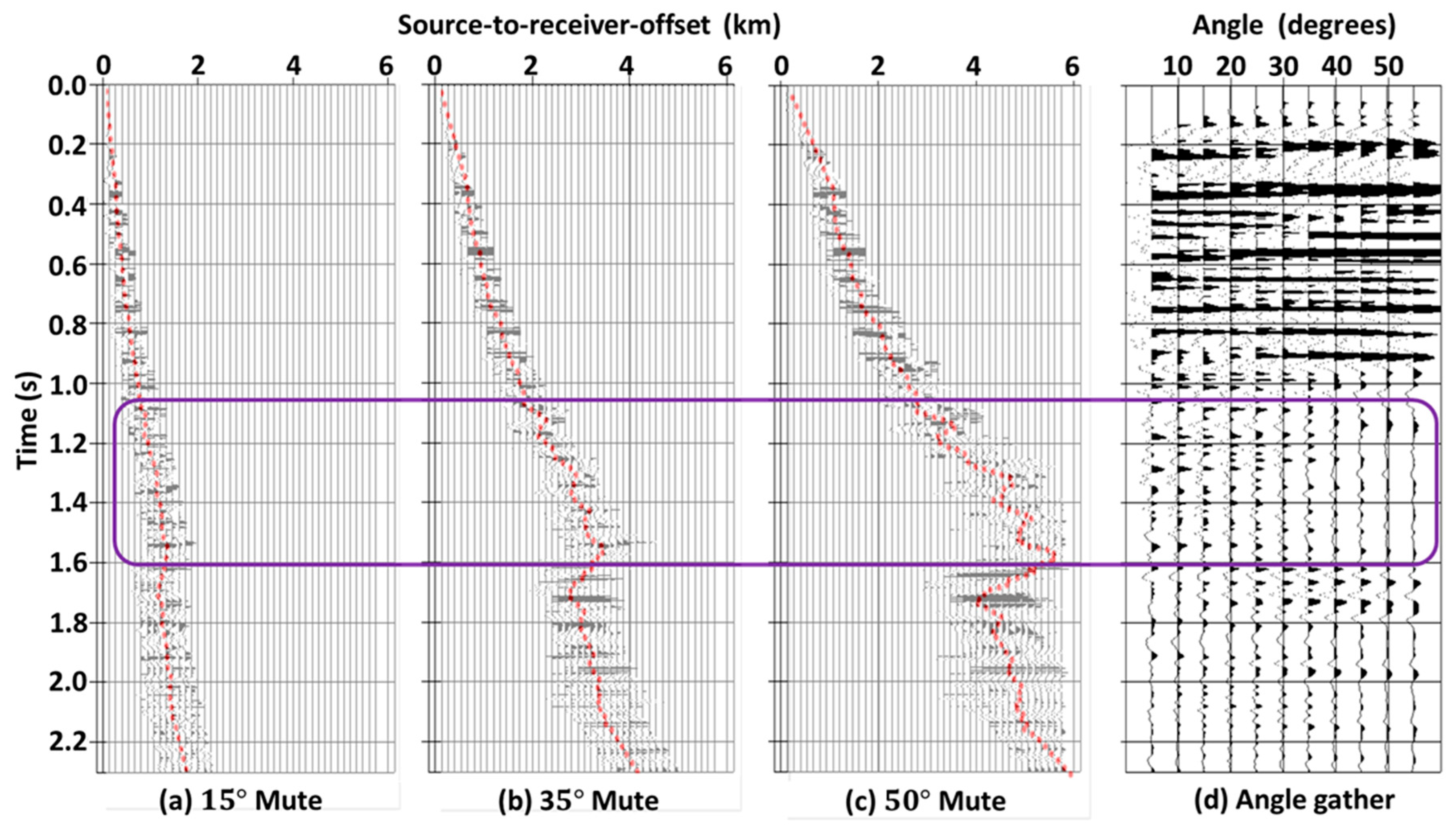
Because seismic data are band-limited, the contribution of each $p$ or $\theta$ does not come precisely from the source–receiver offsets obtained from Equation (3) or Equation (5) but rather a range around them, which lies within the Fresnel zone. This Fresnel zone is given as the quarter wavelength of the dominant seismic frequency on either side of these constant $p$ or $\theta$ trajectories [55,56]. Partial stacking of the $x-t$-domain traces within these Fresnel zones along either constant $p$ or $\theta$ trajectories is the process of slant stacking [57], and the Fresnel zones within which such partial stackings are performed are called the ray parameter mute or angle mute patterns depending on whether they are along constant $p$ or constant $\theta$. Because AVA computes data in the $\theta -t$ domain, here, we illustrate slant stacking for $x-t$-to-$\theta -t$ transformation. We must, however, emphasize that a similar transformation can be performed using constant ray parameters leading to $x-t$ to intercept time/ray parameter ($\tau -p$)-domain transformation. In Figure 6a–c, we show the angle mutes for 15$°$, 35$°$, and 50$°$ incidence angles, along with the smoothed versions of their corresponding constant angle trajectories (dashed red curves). The original (unsmoothed) versions of these smoothed trajectories are presented in black, blue, and red in Figure 5c. The reason for showing the smoothed trajectories instead of the exact ones in Figure 6a–c is not only for clarity but also for a practical reason. Although we compute the constant angle trajectories in Figure 5c from well log $V_P$, in practice, it is only possible to do this at the well locations. For locations away from the wells, the best way to compute them is using the velocities estimated from a velocity analysis or a similar process, and they would be like the ones shown as dashed red curves in Figure 6a–c. The angle mutes shown in Figure 6a–c are the portions of the seismic data in Figure 5c that lie within the Fresnel zones centered around each smoothed constant angle trajectory (dashed red curves). Stacking all live traces within each angle mute is the angle-domain trace for the given angle, and partially stacking the NMO-corrected offset traces along the Fresnel zone for different incidence angle trajectories is the offset-to-angle ($x-t$-to-$\theta -t$) transformation, shown in Figure 6d for incidence angles ranging from 5° to 55° in steps of 5°.

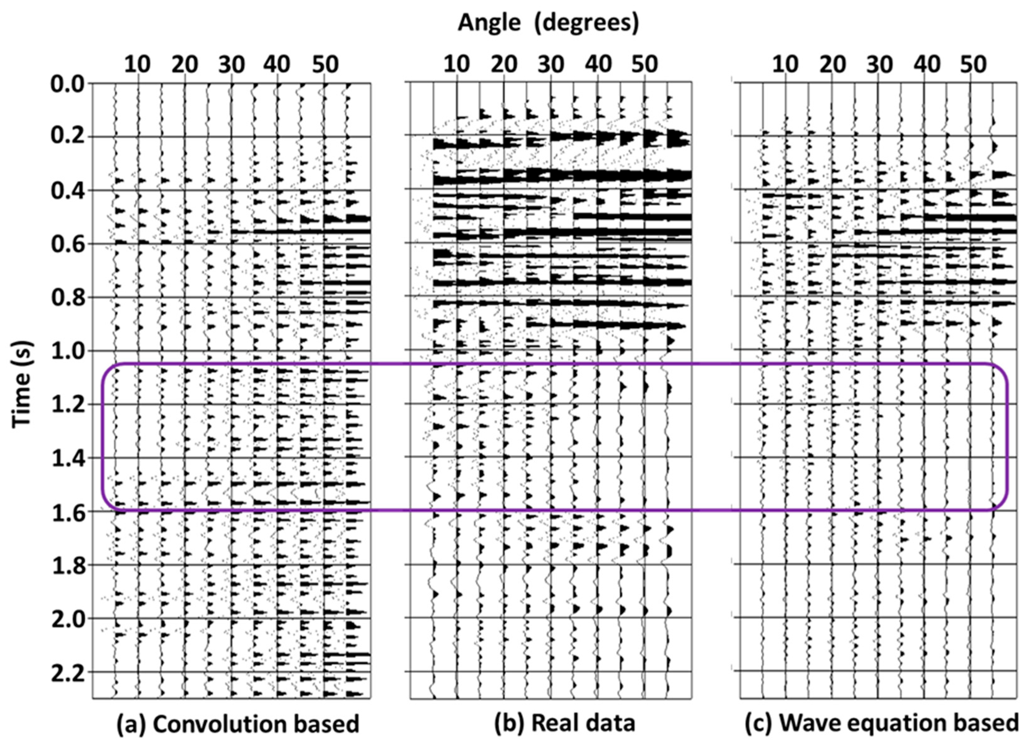
In Figure 7, we compare the real angle gather from Figure 6c with the synthetic angle gather computed from convolution and the wave equation. Figure 7a presents the synthetic angle gather computed using convolution (Equation (1)). Figure 7b presents the angle gather computed from real seismic data via partial stacking, and it is identical to the one shown in Figure 6c. Finally, Figure 7c presents the synthetic angle gather computed from the same 1D wave equation method used to compute the synthetic data in Figure 3b,c.

We now concentrate on the zone lying approximately within the 1.05–1.6 s time window and marked by purple boxes in Figure 5, Figure 6 and Figure 7. It is noticeable in the real $\theta -t$-domain data (Figure 6d and Figure 7b) that, although there are strong reflection amplitudes for $\theta \ge 40°$ above and immediately below 1.05–1.6 s, they appear to be anomalously low within this window. Note in Figure 5b that this 1.05–1.6 s time window is characterized by low velocity, which is then followed by an increasing velocity with a steep gradient between 1.6 and 1.7 s. In addition, the zone above 1.05–1.6 s is characterized by an increasing velocity zone with a moderately steep gradient (~0.3–0.7 s), followed by a zone with an approximately constant velocity (0.7–1.05 s). This scenario is like the four-layer example in Figure 2, as explained below:

• The high velocities above 1.05 with a positive gradient in the 0.3–0.7 s window cause the rays to bend like the black and green ray paths in layers 1 and 2. So, the rays bend successively away from the normal and eventually reach the turning point for large angles.
• The low-velocity zone of the 1.05–1.6 s time window is analogous to layer 3 in Figure 2 and behaves like the blue ray path shown in this figure. So, the rays within this zone turn in the reverse direction and cause the offsets needed for $x-t$-to-$\theta -t$ mapping to be very high. This effect is especially evident in the $50°$ angle mute, as shown in Figure 6c. From these angle mutes (Figure 6a–c), the offsets needed for $x-t$-to-$\theta -t$ mapping for these zone appear to be present in the data. However, because the rays needed for $x-t$-to-$\theta -t$ mapping for $\theta \ge 40°$ within this zone reach the turning point due to the high velocities above 1.05 s, $x-t$-to-$\theta -t$ mapping for these high angles in this zone is not possible, and, therefore, the reflection amplitudes for these high angles within this zone are anomalously low. This effect is also evident from the low reflection amplitudes in the $50°$ angle mute for the 1.05–1.6 s time window (Figure 6c).
• The ray paths in high velocities below 1.6 s behave like those in layer 4, shown by the purple ray path in Figure 2. Because the angle mutes move in the reverse direction (see Figure 6a–c), the rays needed for $x-t$-to-$\theta -t$ mapping for $\theta \ge 40°$ in this zone do not reach the turning point caused by the high-velocity layers above 1.05 s, and, consequently, the reflections for these high angles are visible.

Now, in the $\theta -t$ domain, the synthetic data computed from the convolution (Figure 7a) of all high-angle ($\theta \ge 40°)$ reflections within the entire time window, including the 1.05–1.6 s window, are visible. The wave equation synthetics (Figure 7c), however, model them like they are on real data. Like real data, high-angle reflections are visible above 1.05 s and below 1.6 s, and they are low in the 1.05–1.6 s window. Although not perfect, in an overall sense, the wave equation synthetics present a much closer representation of the real data than the convolutional synthetics. This is because the wave equation method incorporates all wave effects, such as the transmission loss, short-period interbed multiple reflections and mode conversions, effects due to ray bending, and directivity, and convolutional synthetics do not. To incorporate these wave effects in an ad hoc sense, AVA inversion methods tend to use angle-dependent wavelets, but doing so can only approximately and not exactly correct for these effects. Therefore, using a wave equation method for synthetic computation as the forward modeling engine in Figure 1 is more appropriate than convolution.

Before proceeding further, it is necessary to make a few final remarks regarding the slant stacking procedure of $x-t$-to-$\tau -p$ or -$\theta -t$ mapping. Equations (3) and (5) on which these mappings are based are derived from the traveltime formula given in Equation (2). This equation is a two-term approximation of the infinite Taylor Series expansion of the exact equation [58]. Mallick (1999) [22] demonstrated that applying NMO correction using high-order terms and then applying Equations (3) or (5) provide adequately accurate $x-t$-to-$\tau -p$ or $x-t$-to-$\theta -t$ mapping. Exact mapping of the $x-t$-domain seismic data onto $\tau -p$ or $\theta -t$, however, requires plane-wave decomposition [59]. Such plane-wave decomposition is based on Fourier and Hankel transformations requiring prestack seismic data to be adequately sampled in offset and time. Although the time sampling of the recorded seismic data is generally adequate, the offset sampling is not. The RSU seismic data that we use to compute the $\theta -t$-domain data (Figure 6c and Figure 7b), for example, have an offset sampling of 440 feet (134.112 m), and computing $\tau -p$- or $\theta -t$-domain data via the plane-wave decomposition of such $x-t$-domain data will be spatially aliased and unusable. Therefore, the slant stacking process of partially stacking over angle or ray parameter mutes is the most practical choice for mapping the $x-t$-domain data onto the $\theta -t$ or $\tau -p$ domain. Finally, the process of computing the angle (or ray parameter) mutes (Figure 6) is based purely on the traveltimes and the velocities derived from them. These traveltime-based procedures provide ray (group) velocities. The reflections, however, are controlled by constant phase directions. For an isotropic elastic medium, the wavefronts are spherical, where the ray and phase directions are identical. For an anisotropic medium, however, they are different. Therefore, the mapping of $x-t$-domain data onto $\theta -t$ or $\tau -p$ using the partial stacking method that we provide is valid for an isotropic medium only. For an anisotropic medium, it is important to account for the difference between the ray and phase directions, which requires a more rigorous process to obtain the constant ray parameter or phase angle trajectories and their corresponding mutes for partial stacking [60,61].

3. Prestack Waveform Inversion with Genetic Algorithm Optimization

The details of GA-based PWI can be found in Mallick (1995, 1999) [21,22]. For completeness, here, we briefly summarize the implementation aspects of the method. Figure 8 shows the modification of the general seismic inversion workflow in Figure 1 for GA-based PWI. In Figure 8, we use the same color-coding convention as in Figure 1, with the input modules shaded in green, the forward modeling engine used to compute synthetic data shaded in orange, the models modifying via GA optimization shaded in yellow, the iterative process of switching between forward modeling and optimization via matching and eventually entering the output modules shaded in blue, and the output modules shaded in purple. As we can see in Figure 8, there are two inputs to the GA-based PWI, (1) prestack seismic data and (2) the initial population of models of size $N_{pop}$. The prestack seismic data are the relative amplitude-preserved $x-t$-domain data without GSC and NMO. For isotropic elastic inversion, the initial model population consists of the depth-domain models of $V_P,V_S$, and $\rho$, which can be generated in several ways. For example, by taking the initial $V_P,V_S,\rho$ models and specifying a search window around each one, a random population of $N_{pop}$ models can be generated such that the $V_P,V_S$, and $\rho$ at any depth sample can take any random value within their specified search bounds for that sample. Alternatively, in the presence of well logs with borehole measurements of $V_P,V_S$, and $\rho$, we can use the well log data, define a prior distribution, and draw $N_{pop}$ models of $V_P,V_S$, and $\rho$.

Using each $V_P,V_S$, and $\rho$ model, we use a 1D wave equation for the forward modeling engine and compute a set of $N_{pop}$ synthetic (predicted) seismic data, either in the $\theta -t$ or $\tau -p$ domain. This 1D wave equation modeling is the same as the method used to compute the synthetic seismic data shown in Figure 3, besides the fact that we compute them in the $\tau -p$ or $\theta -t$ domain instead of the $x-t$ domain. Details of this 1D wave equation forward modeling can be found in Mallick and Frazer (1987, 1988, 1990, 1991) [50,51,52,53], and, for completeness, we provide a brief overview in Appendix A. From each $V_P$ model, we also obtain observed (real) $\theta -t$- or $\tau -p$-domain data via a partial stacking process that we previously discussed (Figure 5, Figure 6 and Figure 7). After computing the synthetic data and generating the observed data by partial stacking, we then match each set of observed data with the corresponding set of synthetic data to compute the objective for each of the $N_{pop}$ models. For the GA, it is convenient to cast optimization as maximization. We therefore compute the objective $y_k$ for each model $k=1,2,\dots ,N_{pop}$ as normalized cross-correlations, given as

$$y_k={\displaystyle \frac{1}{N_t{N}_{\theta }}}{\sum }_{i=1}^{N_t}{\sum }_{j=1}^{N_{\theta }}{\displaystyle \frac{2S_{ij}{D}_{ij}}{S_{ij}^2+D_{ij}^2}}.$$

(6)

In Equation (6), $N_t$ and $N_{\theta }$ are the number of time and angle (or ray parameter) samples in the observed and synthetic data, respectively, and $S_{ij}$ and $D_{ij}$ represent the synthetic and observed data with $i=1,2,\dots ,N_t$ and $j=1,2,\dots ,N_{\theta }$, respectively.

Having computed the objective $y_k$ for each model $k$, the next step is a convergence check and making the decision whether to continue iterating or exit. However, before discussing this convergence check, it is first necessary to discuss the process of GA optimization, shown in yellow boxes in Figure 8. In the GA, the models are modified using four fundamental processes: (1) reproduction (tournament selection), (2) crossover, (3) mutation, and (4) elitism. Prior to invoking these four fundamental processes, the computed objectives are first scaled using a suitably chosen scaling function. Stoffa and Sen (1991) [20] and Mallick (1995, 1999) [21,22] provided details of how to perform this scaling for prestack seismic inverse problems. The purpose of this scaling is to regularize the computed objectives such that quick convergence to a local optima instead of achieving the target of reaching the desired global optimum (or optima) is avoided [62]. In reproduction, the models are simply reproduced in proportion to their scaled objective values. So, the models with high objective values are reproduced more, and those with low objective values are reproduced less or not reproduced at all. From the original $N_{pop}$ models, reproduction produces a new population of the same size, in which some models from the original population are repeated once or more than once, and some others are eliminated. In crossover, two members from the reproduced population are randomly chosen as parents, and their model contents are partially swapped to produce two children. For a population of size $N_{pop}$, performing $N_{pop}/2$ crossovers would thus produce an $N_{pop}$ child population from an $N_{pop}$ parent population. Crossover is generally performed with a given crossover probability $P_{cross}$. After choosing the parents, a coin is tossed for each model parameter, with the chance of obtaining heads set to $P_{cross}$. If the outcome of the coin toss is heads, only then is the crossover between the parents for the given model parameter performed; otherwise, they are left as they are. In mutation, each model parameter of the entire child population is sequentially visited and changed with a mutation probability $P_{mut}$. Following crossover and mutation, the objectives of the new (child) population are computed, scaled, and compared with their corresponding parents. Then, with a probability of elitism $P_{elit}$, the best two out of each pair of parents and their (mutated) children are chosen to advance to the next generation. Performing such $N_{pop}/2$ elitism operations advances the $N_{pop}$ members of the old generation to $N_{pop}$ members of the new (next) generations. This process of advancing to the new generation continues until it reaches one of the stopping criteria (see Figure 8).

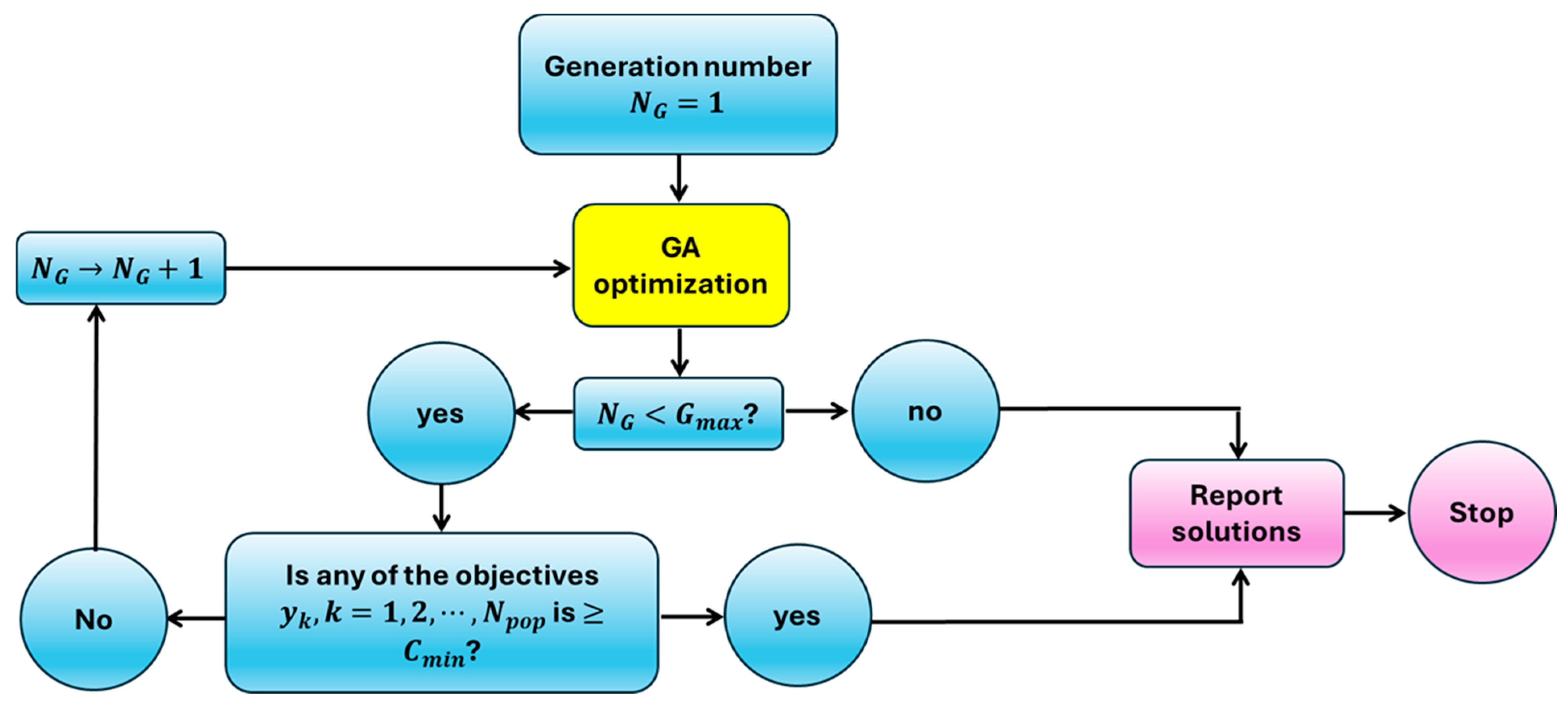
We use Figure 9 to illustrate the setting up of the stopping or convergence criteria for the GA, which is controlled by two parameters: (1) $G_{max}$ and (2) $C_{min}$. $G_{max}$ is the maximum number of generations, and $C_{min}$ is the minimum correlation value between the observed and predicted (synthetic) data ($D_{ij}$ and $S_{ij}$ in Equation (6)) to be attained in the optimization process. After advancing to the new generation, $N_G$, we first check whether $N_G=G_{max}$. If yes, we stop iterating and report the solutions. However, if $N_G<G_{max}$, we check whether any of the computed objectives ($y_k, k=1,2,\dots ,N_{pop}$) $\ge C_{min}$. If yes, we exit iteration to report the solutions. However, if none of the computed objectives are $\ge C_{min}$, we then advance the generation and continue iterating. The choice of GA parameters ($N_{pop},G_{max}$, and $C_{min}$) and the probabilities of crossover, mutation, and elitism ($P_{cross},P_{mut}$, and $P_{elit}$) are data-dependent. However, Jia et. al. (2021) [17] conducted thorough testing of these parameters and found that the following choices generally work for a wide set of real seismic data: $N_{pop}=80$; $G_{max}=400$; $C_{min}=0.95$; $P_{cross}=0.6$; $P_{elit}=0.9$; and $P_{mut}=0.1$ for the first 1/10th of $G_{max}$ (generations 1–40) and 0.001 for generations 41 to 400. In our applications (shown below), we use this recommended set of parameters.

Besides the fundamental steps in Figure 8 and Figure 9, inverting real seismic data using GA-based PWI requires the consideration of other aspects. These aspects include (1) the method used to generate the random model population, (2) the methods used to preserve population diversity, and (3) the different methods used for parameter coding to drive GA optimization. The details of these aspects, including sensitivity analyses of different parameters, can be found in [63]; we do not repeat them here.

4. Inversion Setup

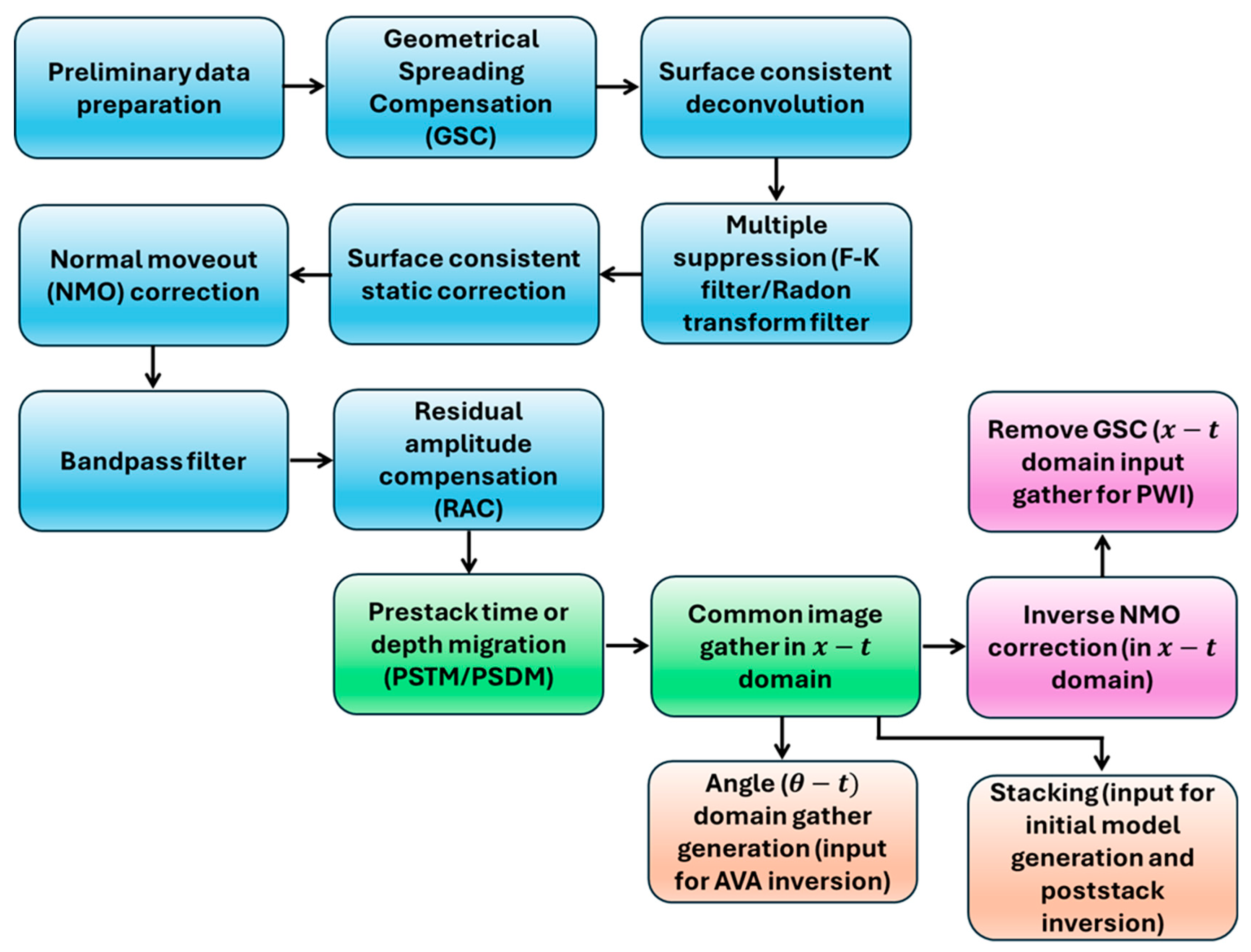
In Figure 5, Figure 6 and Figure 7, we use a single $x-t$-domain prestack gather and the corresponding well log ($V_P$ only) from the RSU area and demonstrate $x-t$-to-$\theta -t$ mapping. Here, we provide the procedures for setting up both AVA inversion and PWI using 3D RSU seismic and RSU #1 well log data. The RSU seismic data volume is acquired with 245 inlines and 247 crosslines spanning an area of approximately 25 miles² (64 km²). The inline direction is oriented west to east, and the crossline direction is oriented south to north. The first step in setting up any inversion run is the processing of the raw seismic data using a relative amplitude-preserved (RAP) data processing workflow. In Figure 10, we provide this workflow. The modules shaded in blue in Figure 10 are the recommended RAP processing steps practiced in the seismic industry for AVA analysis. Detailed descriptions of these steps can be found in Resnick (1993) [56]. To this recommended RAP processing, we add prestack time or depth migration, shaded in green in Figure 10. By moving the image locations for all source–receiver pairs to their reflection points, the $x-t$-domain common image gathers from migration is a crucial step to approximately validate the inherent 1D assumptions of both AVA and PWI. Additionally, by focusing the image, this process also improves the signal-to-noise ratio, which, in turn, lets both AVA inversion and PWI quickly converge and save a lot of computational expense. For a relatively simple subsurface geology, applying prestack time migration (PSTM) is adequate. However, when the geology is complex, prestack depth migration (PSDM) is more appropriate than PSTM. It is also important to note that the migration method, either PSTM or PSDM, must be an amplitude-preserving process. There are a variety of true-amplitude PSTM and PSDM methods (Yilmaz, 2001 [54]) that can be applied depending on the complexity of the subsurface geology. The geology of the RSU area is simple, with gentle southwest-to-northeast trending dips not exceeding $3-4°$. We therefore apply a Kirchoff PSTM method (Yilmaz, 2001 [54]) for migration. For AVA inversion, we convert the $x-t$-domain image gathers into the angle ($\theta -t$) domain via partial stacking, as described above in Figure 5, Figure 6 and Figure 7. We also stack the $x-t$-domain migrated gathers to produce the stacked seismic data volume. As we explain below, this stacked data volume is needed to generate the initial model. Additionally, this volume can also be used as input for poststack inversion. Generating $\theta -t$-domain gathers by partial stacking and using the process of stacking to generate zero-offset traces are parts of the recommended RAP processing. However, because we generate them in our workflow from the common image gathers after migration, we show these modules in a different (peach) color in Figure 10. While AVA inversion works on $\theta -t$-domain data, the input to PWI is $x-t$-domain prestack data without any NMO or GSC. We therefore remove the NMO correction and reverse the GSC from the common image gathers to prepare data as input to PWI, and, in Figure 10, we show these steps in purple.

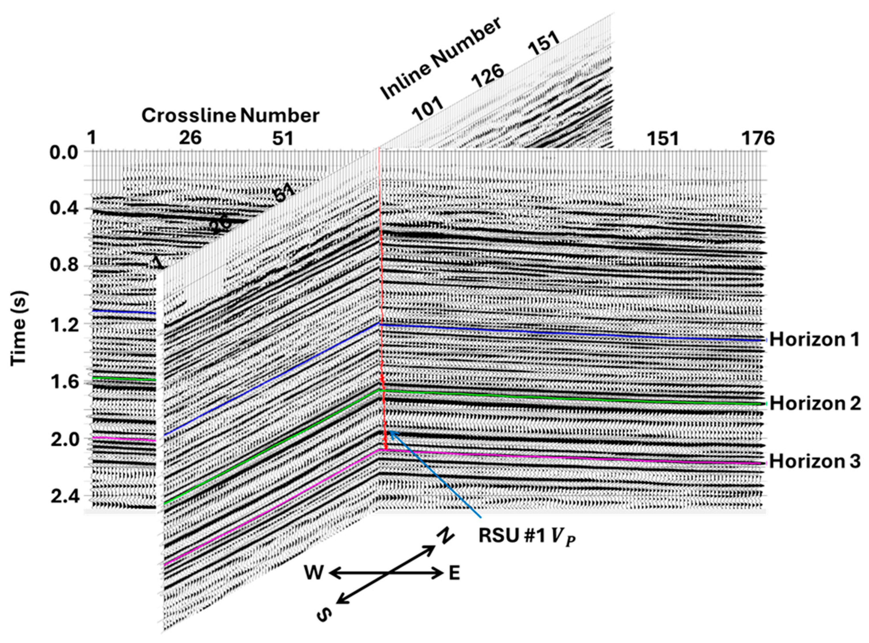
Out of the entire 3D data volume, 176 inline and 176 crossline locations have enough offsets needed for prestack inversion. In Figure 11, we show the stacked seismic data after RAP processing for one inline (IL-74) and one crossline (XL-77), which intersect one another at the location of the RSU #1 well.

Following RAP processing and setting up the input data, the next step in seismic inversion is generating an initial model. This initial model generation requires three steps: (1) importing well logs ($V_P,V_S,\rho$) at the proper location (or locations) of the seismic data and tying them to the seismic data; (2) interpreting horizons on the stacked seismic data; and (3) interpolating the well logs over the interpreted horizons to provide the initial models of $V_P,V_S$, and $\rho$. Once the initial model is generated, an appropriate forward modeling method is needed to compute the synthetic data, match them to the observed data, and iteratively modify the model via optimization (see Figure 1 and Figure 8). Because seismic data are band-limited, it is also necessary to provide an appropriate wavelet for the synthetic data computation for both AVA and PWI. This wavelet estimation is an integral part of the seismic-to-well tie. Below, we use RSU data to provide the steps for generating the initial model, estimating the wavelet, and setting up parameters for both AVA inversion and PWI.

Step 1, importing well logs, well-to-seismic tie, and wavelet estimation: The RSU area had a single well (RSU #1) with a suite of well log measurements, including $V_P,V_S$, and $\rho$. The location of the RSU #1 well corresponded to the intersection of IL-74 and XL-77, and the well logs were in the depth domain with the depths measured from Kelly bushing at an elevation of 6679 feet (2036 m) above the mean sea level (MSL). The RSU seismic data, however, were processed with a reference datum of 7500 feet (2286 m) above the MSL. After importing the $V_P,V_S$, and $\rho$ logs from the RSU #1 well at its proper location, for the well-to-seismic tie, we bulk-shifted them such that their measured depths corresponded to the depths from the seismic datum. We then converted the depth-domain well logs into two-way P-wave times. The starting and ending depths of the RSU #1 well logs were 400 and 4200 m, respectively, after bulk shifting to the seismic datum. Starting with the depth domain $V_P$ between 400 and 4200 m from the RSU #1 well log, we obtained the time-domain $V_P$ model that optimally flattened the prestack seismic data for NMO. This time-domain $V_P$ is shown as the interval velocity in Figure 5b, in which the actual well log spans a time interval between 0.3 and 2.1 s, and the overburden $V_P$ values above 0.3 s and below 2.1 s were estimated from velocity analysis. The prestack data shown in Figure 5a were optimally NMO-corrected (Figure 5c) using the $V_P$ model in Figure 5b. Therefore, the interval $V_P$ in Figure 5b is a well-to-seismic-tied well log in the time domain. Using the same depth-to-time conversion, we also obtained our well-to-seismic-tied RSU #1 $V_S$ and $\rho$. For outside the well log time interval (<0.3 s and >2.1 s), we computed $V_S$ by setting $V_S={\displaystyle \frac{V_P}{2}}$, and we computed $\rho$ from Gardner’s power law equation as $\rho =\alpha V_P^{\beta }$ [64]. In Figure 11, we overlay the RSU #1 $V_P$ at its proper location after the depth-to-time conversion and well-to-seismic tie.

Following well-to-seismic tie, we used the stacked seismic data and the well-to-seismic-tied $V_P$ and $\rho$ for wavelet estimation. If stacked seismic data are represented as $S\left(t\right)$, the zero-offset (normal incidence) reflection coefficient is represented as $R_0\left(t\right)$, and $W\left(t\right)$ is the wavelet to be estimated; then, from the convolution equation (Equation (1)), we write

$$S\left(t\right)=W\left(t\right)\ast R_0\left(t\right).$$

(7)

By Fourier-transforming Equation (7) into the frequency ($\omega$) domain and using the convolution theorem [65], we can write the frequency-domain version of Equation (7) as

$$S\left(\omega \right)=W\left(\omega \right)R_0\left(\omega \right).$$

(8)

Equation (8) allows us to estimate the frequency-domain wavelet $W\left(\omega \right)$ as

$$W\left(\omega \right)={\displaystyle \frac{S\left(\omega \right)}{R_0\left(\omega \right)+N_W}}.$$

(9)

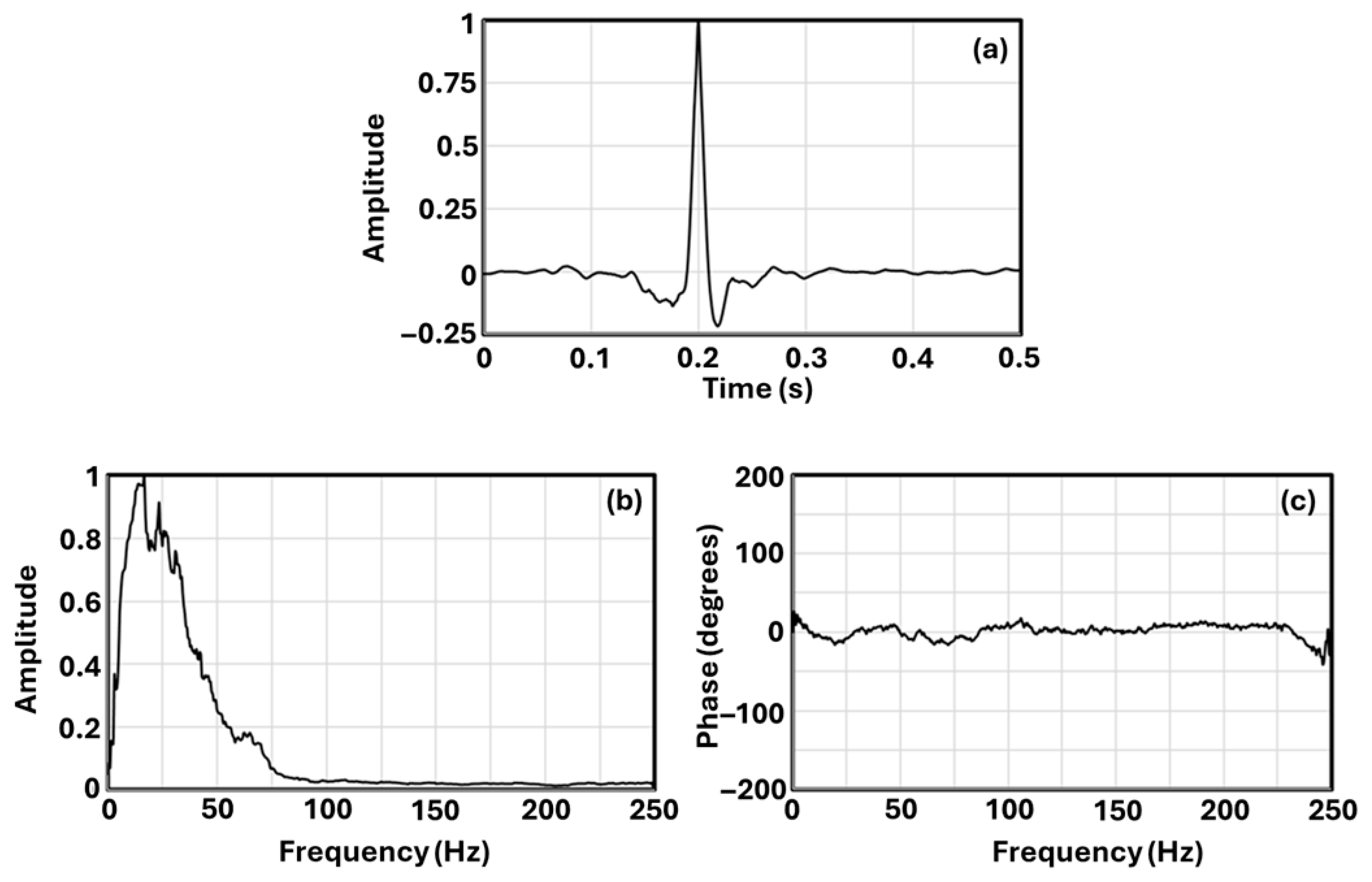
The parameter $N_W$ in the denominator of equation 9 is the white noise added for the stability of the wavelet estimation, typically computed as a fraction of the RMS value of the amplitude spectrum of $S\left(\omega \right)$. Figure 12 shows the estimated wavelet for the RSU seismic data using the above procedure in both the time and frequency domains with 10% white noise ($N_W=0.1)$. The wavelet estimation shown in Figure 12 is from stacked seismic data. For PWI, using such a single wavelet is adequate. To handle the complex effects of wave propagation and other issues that we discussed above, AVA requires angle ($\theta$)-dependent wavelets. These $\theta$-dependent wavelets can be easily computed using the same process by replacing $R_0\left(t\right)$ in Equation (7) with $R_{\theta }\left(t\right)$, where $R_{\theta }\left(t\right)$ is the reflection coefficient for the incidence angle $\theta$.

Step 2, horizon interpretation: Geophysical inversions, like many optimization problems in applied sciences and engineering, are nonunique problems. Restricting to isotropic seismic inversion, nonuniqueness means that, given the observed seismic data, there could be many models within the entire model space of $V_P,V_S$, and $\rho$ that can fit the observation equally well. Out of many such solutions, our objective is to find a solution that is consistent with the local geology of the area of interest. Finding this geologically consistent model from seismic inversion requires estimating a geologically consistent initial model. Starting with such an initial model, seismic inversions using gradient-based local optimization can then quickly find the desired model. Because our PWI is GA-based global optimization, it does not, in theory, require such a geologically consistent initial model. However, the GA runtime required to estimate a geologically feasible model is prohibitively expensive if we start from an initial model that is not consistent with the local geology. Therefore, for practical implementations, providing a good geologically consistent initial model is also necessary for PWI.

The first step in initial model generation is to interpret horizons from the stacked seismic data. These horizons must be carefully interpreted. As a rule of thumb, the number of interpreted horizons should be limited as much as possible such that they follow the local geology but do not put too much bias on the resulting model. We therefore set the limit to only three horizons, and, in Figure 11, we show them as “Horizon 1”, “Horizon 2”, and “Horizon 3”. The interpretation of horizons is a fully automated process in most seismic inversion software platforms. After automatic picking, it is, however, necessary to scan through the entire data volume and ensure that they are consistent throughout. In our application, we first interpret these three horizons on IL-74 and scan through every 10th inline and crossline location to ensure that they are consistent throughout the data volume.

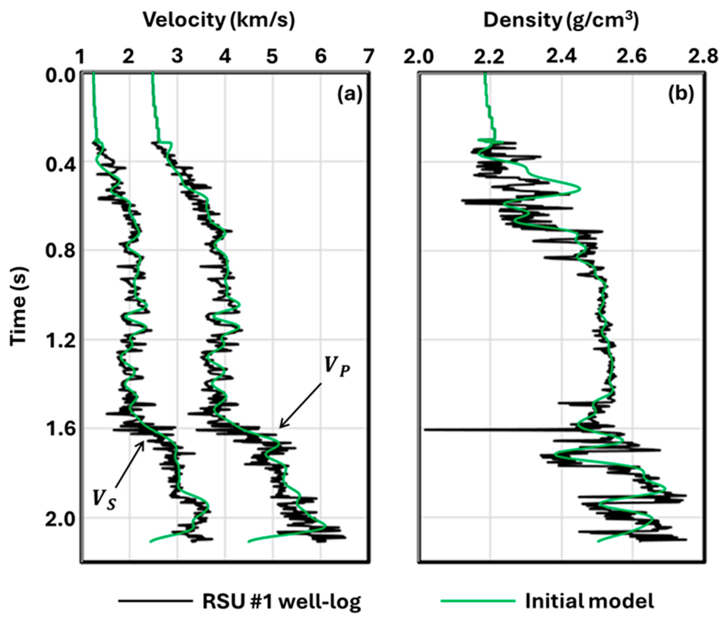
Step 3, initial model generation: Following horizon interpretation, the initial model is generated by interpolating the low-frequency components of the imported well logs over the interpreted horizons. In our application, we filter the time-domain RSU #1 $V_P,V_S$, and $\rho$ logs using a 10–15 Hz high-cut filter and interpolate them over the three horizons as the estimate of the initial model. Figure 13 compares the low-frequency model with the actual RSU #1 well logs, and Figure 14, Figure 15 and Figure 16 show the interpolated initial model for IL-74 and XL-77.

5. AVA Inversion

Starting from the initial models of $V_P,V_S$, and $\rho$ (Figure 14, Figure 15 and Figure 16), AVA inversion can be performed using the generalized prestack inversion workflow in Figure 1, where, in each iteration step, the forward synthetic computation is the convolution (Equation (1)). After computing the objective from the match between the real and synthetic $\theta -t$-domain gathers, the gradient of the objective is computed and used to update the model in each iteration step. To account for complex wave propagation effects, which we previously discussed, this AVA inversion also uses an angle ($\theta$)-dependent wavelet instead of a single wavelet, as shown in Figure 12. The details of this AVA inversion using the workflow in Figure 1 is given in Hampson et al. (2005) [10], and, in Figure 17, Figure 18 and Figure 19, we provide the estimated $V_P,V_S$, and $\rho$ from AVA inversion for the RSU seismic data along IL-74 and XL-77.

6. Prestack Waveform Inversion

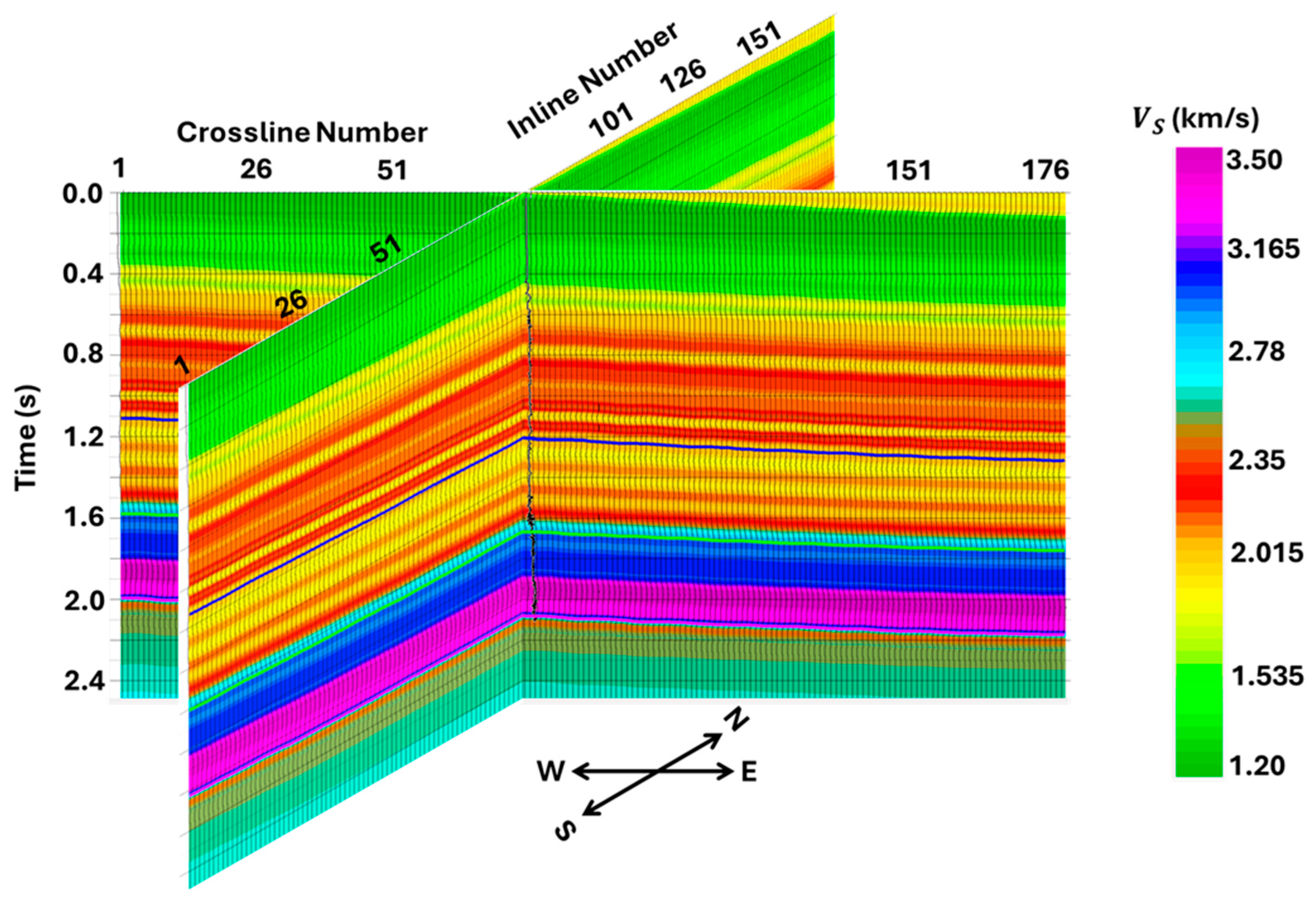
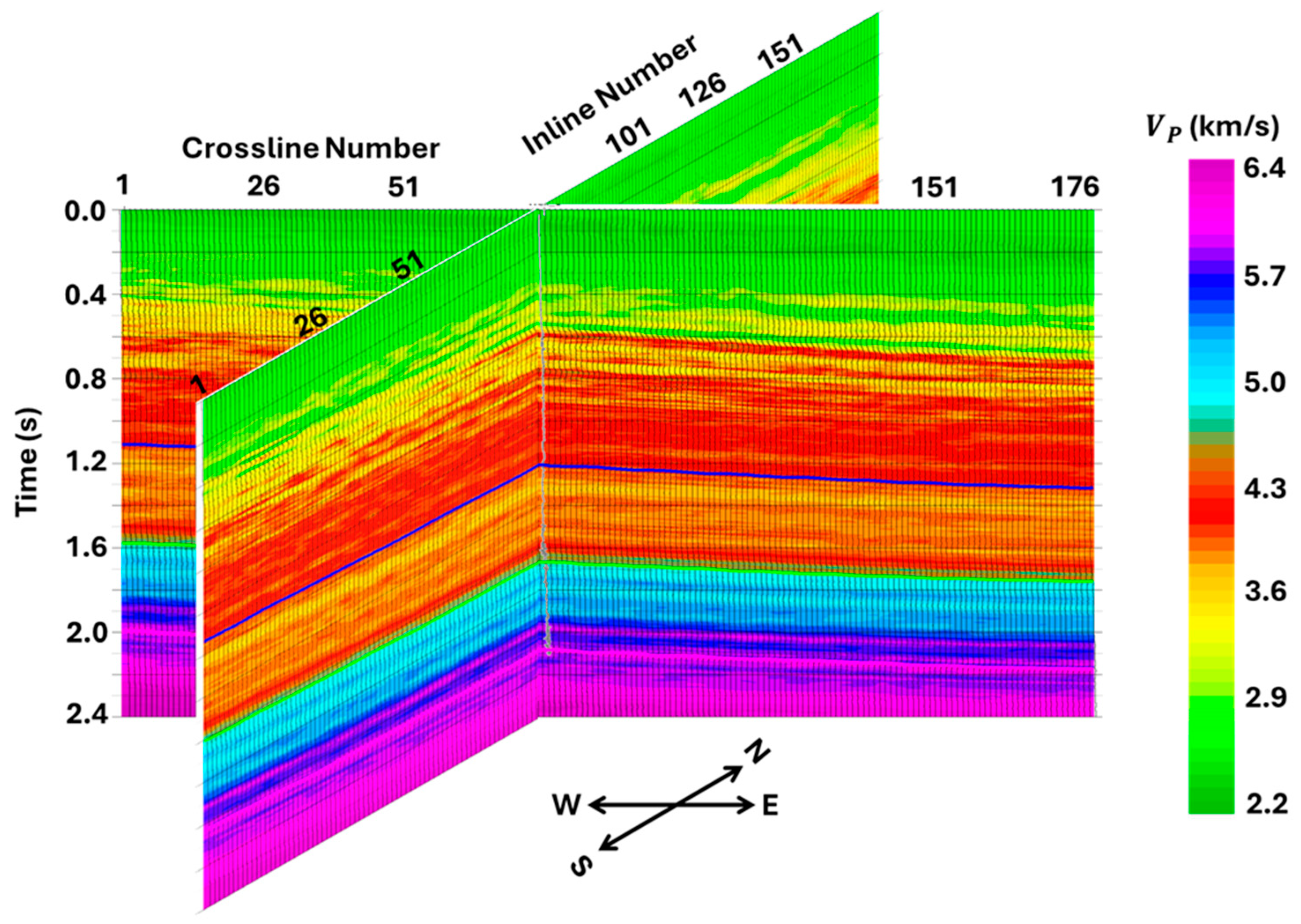
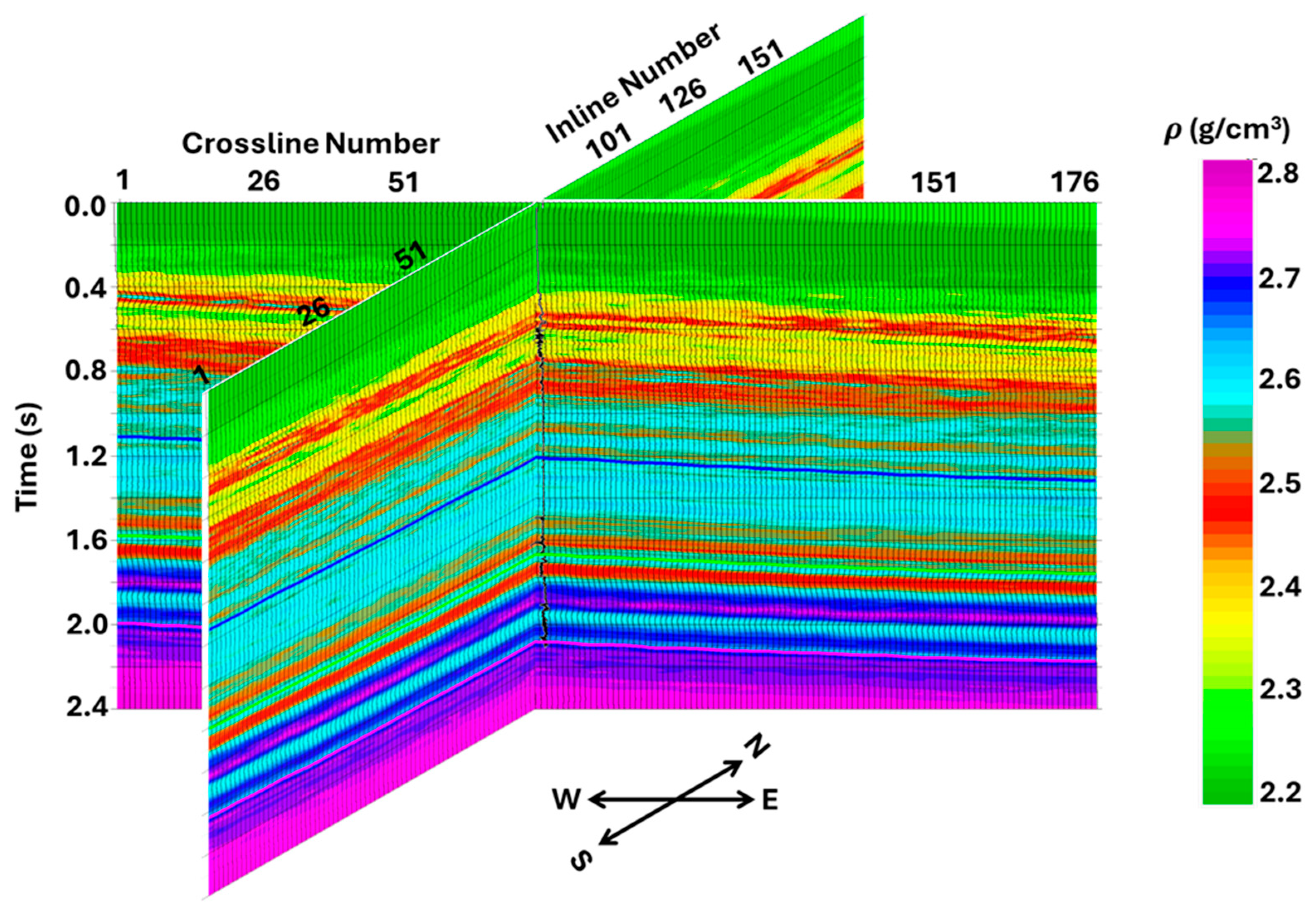
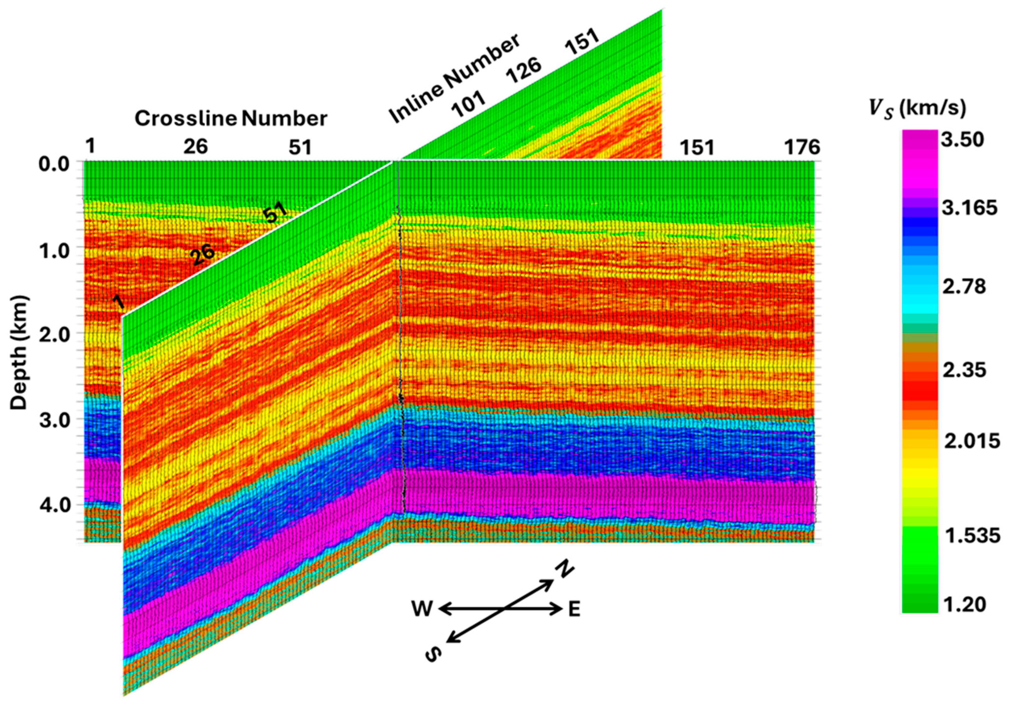
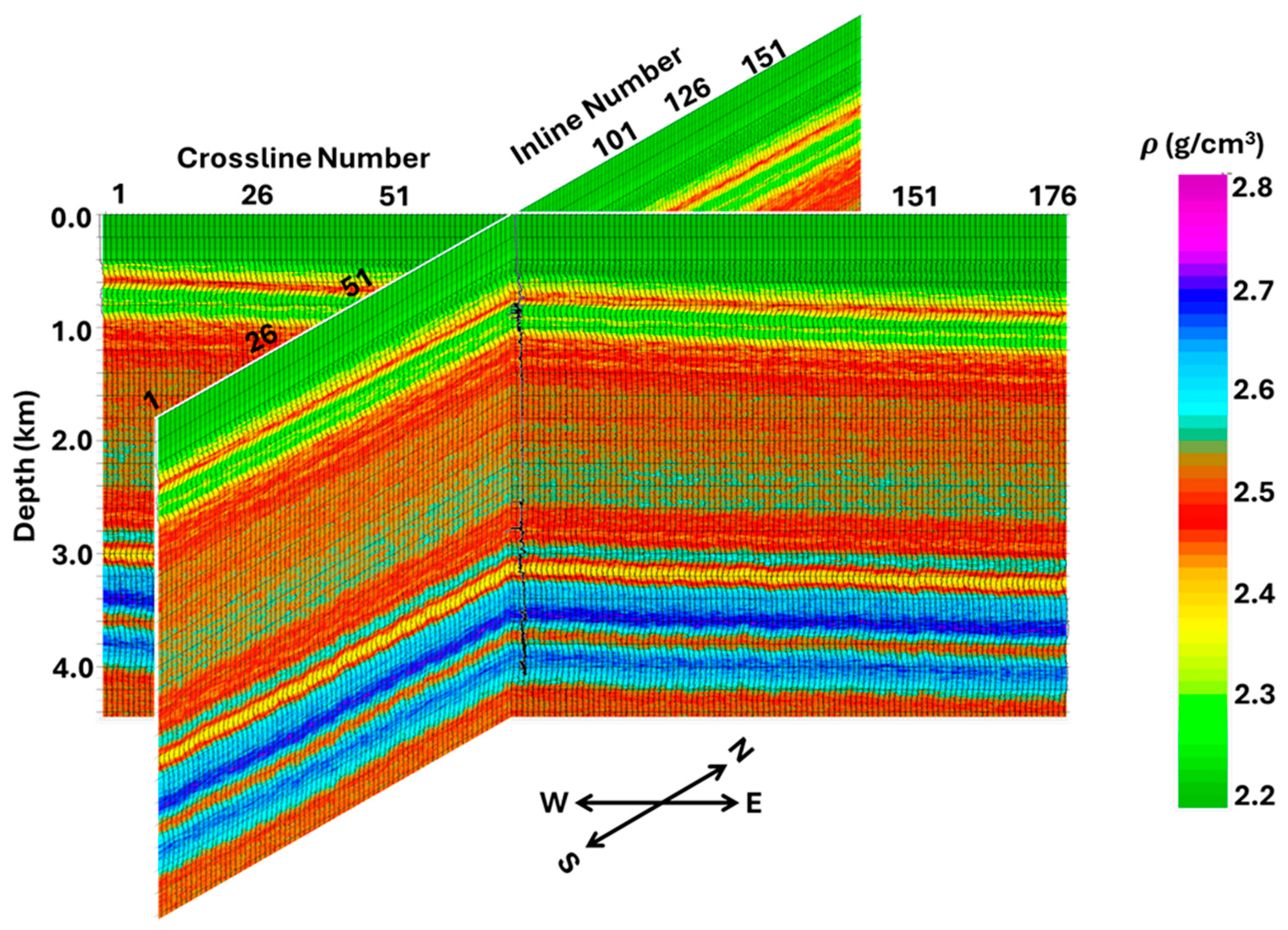
Like AVA inversion, we start from the same initial models of $V_P,V_S$, and $\rho$, shown in Figure 14, Figure 15 and Figure 16 for the GA-based PWI. However, instead of the angle-dependent wavelet, we use a single wavelet, as shown in Figure 12. Additionally, computing wave equation synthetic seismic data requires models in the depth domain instead of in the time domain, and the output is also in the depth domain. We therefore convert the initial time-domain models in Figure 14, Figure 15 and Figure 16 into depth-domain models and iteratively update them using the workflows shown in Figure 8 and Figure 9. The estimated depth-domain $V_P,V_S$, and $\rho$ models from PWI are shown in Figure 20, Figure 21 and Figure 22, respectively.

7. Discussion

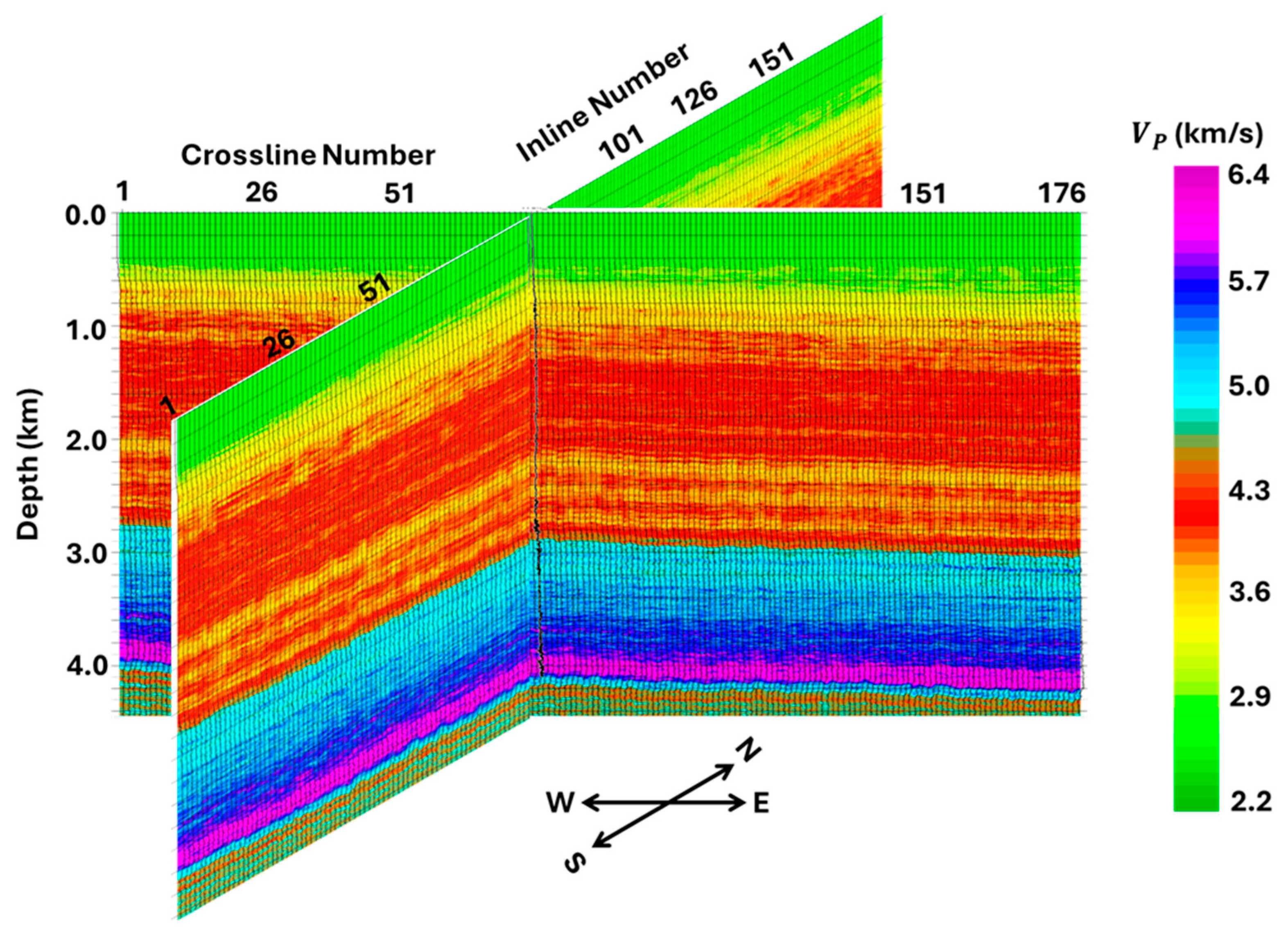
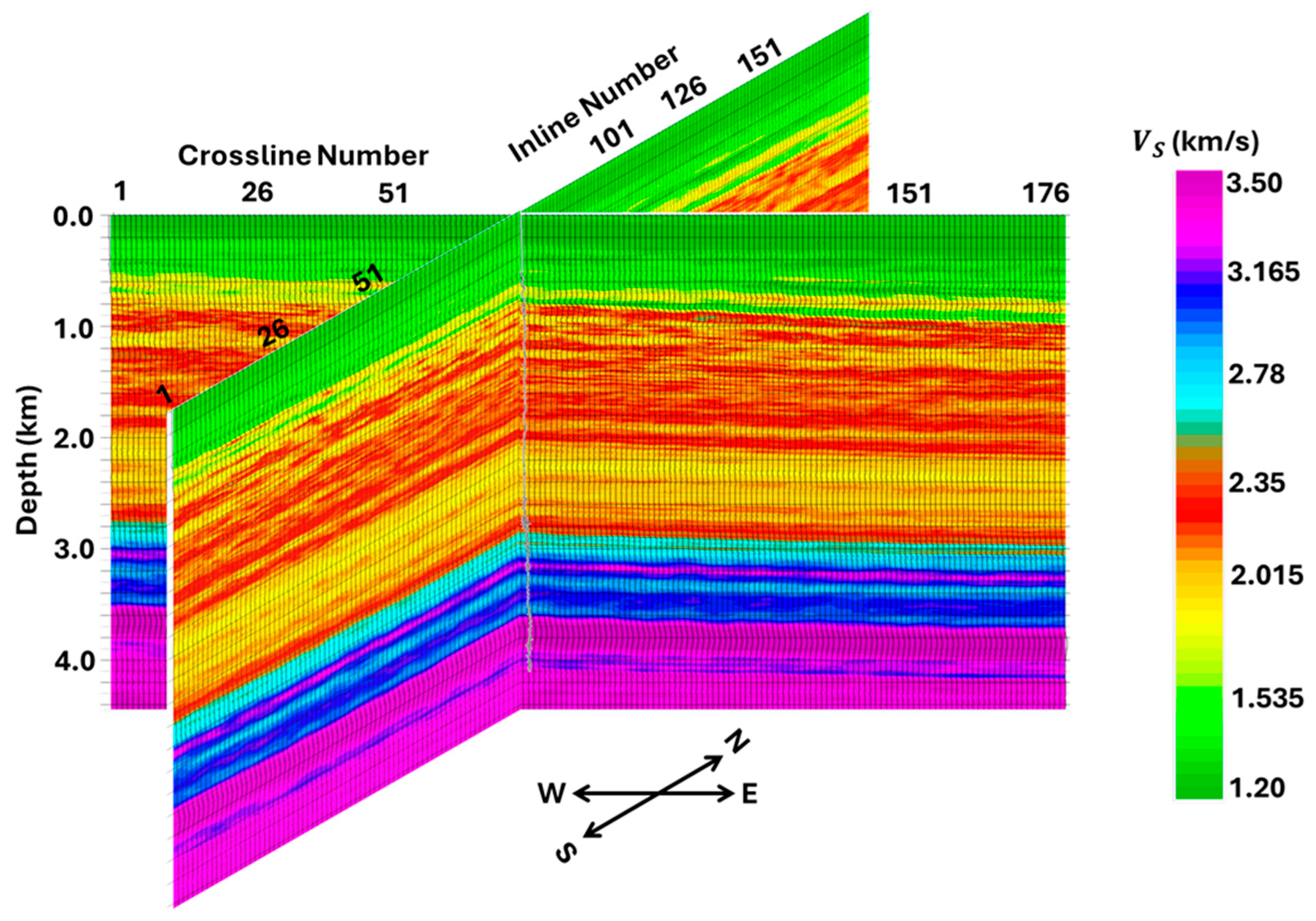
While the models estimated from AVA are in the time domain, those estimated from PWI are in the depth domain. To directly compare the results of these two inversions, we first convert the time-domain models from AVA inversion (Figure 17, Figure 18 and Figure 19) into the depth domain and show them in Figure 23, Figure 24, Figure 25 and Figure 26.

Comparing the depth-domain results from PWI with those from AVA inversion, we observe the following:

• In an overall sense, the inverted $V_P$ and $V_S$ obtained from PWI and AVA inversion have similar features (see Figure 20 and Figure 23, and Figure 21 and Figure 24, respectively).

  ○

  Between 0 and 3.5 km, they can both be subdivided into three velocity zones: (1) 0–0.8 km—a low-velocity (green) zone; (2) 0.8–2.8 km—a slightly higher velocity (yellow to red) zone; and (3) 2.8–3.5 km—an even higher velocity (cyan to blue) zone. Within each of these zones, the PWI-estimated $V_P$ and $V_S$ (Figure 20 and Figure 21) are, however, of a much higher resolution than the corresponding AVA-estimated models (Figure 23 and Figure 24).

  ○

  Below 3.5 km, we observe a major difference between the PWI- and AVA-estimated $V_P$ and $V_S$ models. AVA (Figure 23 and Figure 24) estimates the entire zone below 3.5 km as a high-velocity (blue to purple) zone. PWI (Figure 20 and Figure 21), however, finds two separate zones: (1) 3.5–4 km, with a high velocity (blue to purple), and (2) below 4 km, with a relatively low velocity (cyan to green). Earlier interpretations of the RSU data by Pafeng et al. (2017) [28] revealed that the purple layer, starting from about 3.8 km in both $V_P$ and $V_S$ (Figure 20, Figure 21, Figure 23 and Figure 24), marks the top of the Madison carbonate formation. Additionally, fracture and core analysis studies revealed that the top of this formation is a tight limestone with a high velocity; this is then followed by a dolomitized formation, which is highly fractured with low $V_P$ and $V_S$ [66]. Note that PWI identifies both the high-velocity limestone (~3.8–4 km) and the low-velocity dolomitized zone below 4 km. AVA, however, fails to delineate the dolomitized part of the Madison formation.

• From a quick inspection, the PWI- and AVA-estimated density models (Figure 22 and Figure 25) appear to be different and require further analysis:

  ○

  On the top part (~0–1 km), the PWI and AVA densities are comparable. In the 1–3 km window, the PWI densities have an average value of about 2.5 g/cm³, while the AVA densities average at approximately 2.6 g/cm³. For depths above 3 km, the estimated densities from PWI and AVA are similar. Below 4 km, however, the density drop in the dolomitized part of the Madison formation can be delineated from PWI but not from AVA.

  ○

  In an overall sense, the PWI-estimated density model is of a higher resolution than the AVA-estimated density model.

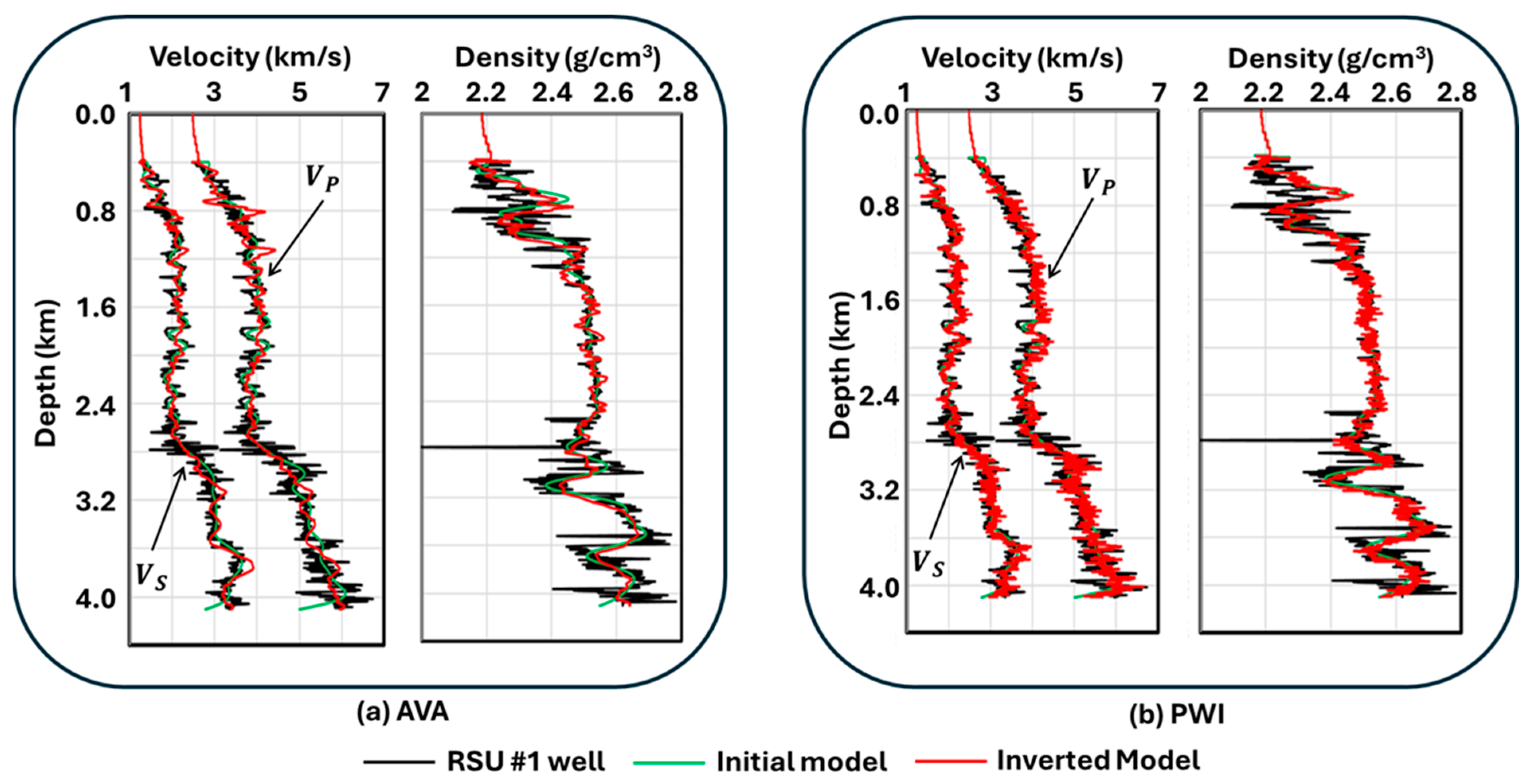
To further analyze the similarities and differences between the PWI- and AVA-estimated models, in Figure 26, we compare the well logs (black curves) and the initial models (green curves) with the models estimated from AVA inversion (red curves in Figure 26a) and PWI (red curves in Figure 26b) at the RSU #1 well location. Clearly, the PWI results are of a much higher resolution than the AVA results. Note in Figure 26a that, although the AVA results are satisfactory in an overall sense, they are of a low resolution. In addition, it fails to accurately predict the well logs in certain zones. However, the PWI results, shown in Figure 26b, are of a much higher resolution than the AVA inversion results. Besides the prediction density in the shallow part, approximately between 0.6 and 0.7 km, the PWI-estimated models almost duplicate the well logs. In addition, the average density in the 1–3 km window is about 2.5 g/cm³, not 2.6 g/cm³, which is more consistent with the PWI-estimated density model (Figure 22) than the AVA-estimated density model (Figure 25).

To illustrate the accuracy of PWI compared with that of AVA inversion, in Figure 27a and b, we compare real stacked data of IL-74 with the synthetic stacked data computed from the estimated $V_P,V_S$, and $\rho$ models from AVA inversion (Figure 27a) and PWI (Figure 27b). We first compute wave equation synthetic seismograms using the estimated models for each CMP location along IL-74 for the same range of source-to-receiver offsets, as they are in the real seismic data. We then compensate the computed synthetic data for geometrical spreading, correct them for NMO, and stack them. It is evident in Figure 27a that there are visible differences between the real stacked data and synthetic stacked data computed from the AVA-estimated model for the entire data range. However, the synthetic stacked data from the PWI-estimated model almost duplicate the real stacked data, and the difference between the two is negligibly small (Figure 27b). Furthermore, in Figure 27c, we compare the cross-correlation between the real and synthetic prestack data computed from Equation (6) along IL-74 and XL-77 for both the AVA and PWI models. Note that, while the average cross-correlations for the PWI-estimated models are about 0.9, those for the AVA-estimated models are much lower, with an average value between 0.5 and 0.6. These cross-correlation values further illustrate the superiority of PWI over AVA inversion.

Despite its superiority, we must admit that PWI is much more computationally demanding than AVA. We ran AVA inversion on a laptop computer with an Intel 10th Generation Core^TM i7 processor, and inverting the entire 3D dataset with 176 inline and crossline locations took about 18 h to complete. Our PWI is fully parallelized, the details of which are thoroughly discussed by Mallick and Adhikari (2015) [27]. Using 100 compute nodes, each with 128 AMD Milan cores, inverting the same data volume using our parallelized PWI required about 36 h. Although these are not direct comparisons, it is still evident that PWI is much more computationally demanding than AVA. We can, however, argue and justify this additional runtime as follows:

• The need to estimate an accurate subsurface model from inversion is vital for all aspects of subsurface reservoir characterization projects. This is also true for hydrocarbon exploration and CCS-related projects. As we shift to non-fossil fuel resources like geothermal energy and hydrogen storage, the need to estimate an accurate subsurface model is vital for optimal energy production from these resources. By conducting thorough qualitative and quantitative analyses (Figure 20, Figure 21, Figure 22, Figure 23, Figure 24, Figure 25, Figure 26 and Figure 27), we clearly demonstrated the superiority of the estimated model from PWI over that from AVA inversion.
  • Referring to the RSU example, RSU data were acquired to characterize the site for delineating potential formations for long-term CO₂ storage. The low-velocity and -density zone within the dolomitized zone of the Madison formation is indicative of fracture porosity and, therefore, a potential storage formation. This fractured zone was clearly delineated by PWI and not by AVA inversion.
  • Such an additional accuracy justifies the preference for running PWI instead of AVA for any reservoir characterization project.
• PWI is currently fully parallelized and optimized for running on CPU-based high-performance computing platforms. The 1D forward modeling methodology implemented in PWI is, however, easily portable to GPU-based platforms. Nowadays, access to high-performance computing, both CPU- and GPU-based, is common. Therefore, our proposed PWI method can be routinely run for future reservoir characterization projects.

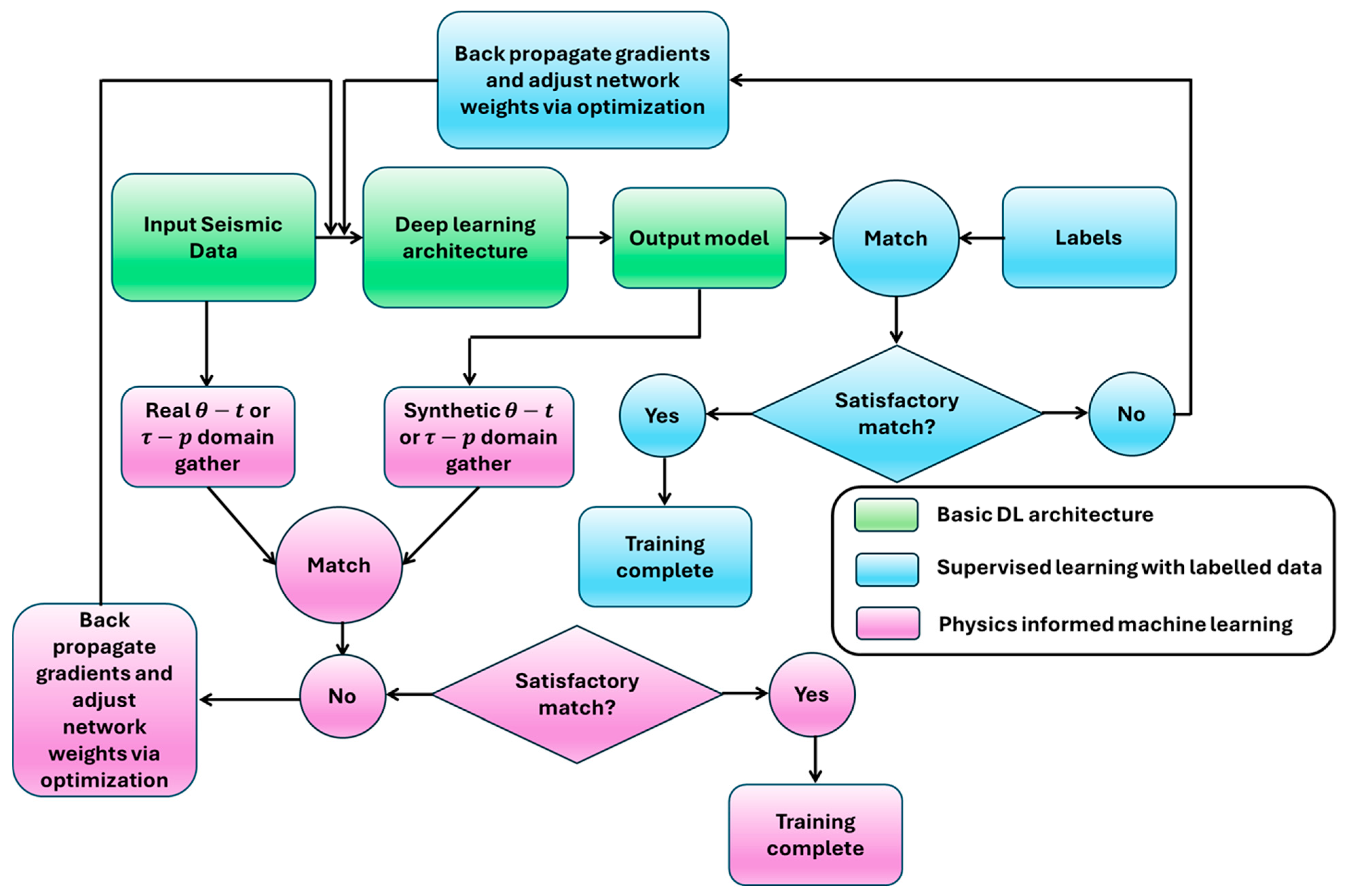
It is, however, worth investigating whether the computational efficiency of PWI can be further improved. Recently, the use of artificial intelligence (AI) technology has revolutionized all fields of applied science and engineering. Using AI for seismic inversion has also been recently investigated [67,68,69,70,71,72,73,74,75,76,77,78,79,80,81,82,83,84,85,86,87,88,89,90,91,92,93,94,95,96,97,98,99,100,101,102,103,104,105,106,107,108,109,110,111,112,113,114,115,116,117,118,119,120,121,122,123,124,125,126,127,128,129,130,131,132,133], a comprehensive account of which can be found in Mallick (2025) [63], and, in Figure 28, we provide an overall vision of how deep learning (DL) can improve the computational efficiency of PWI and other seismic inversion methods. In the modules shaded in green in Figure 28, the input seismic data are fed to a DL architecture, such as a convolutional neural network (CNN), which outputs an estimated model of $V_P,V_S$, and $\rho$. To refine this model by adjusting the network weights, we show two different approaches. The first approach is traditional supervised learning using labeled data, which are shaded in blue. In this approach, we provide the true $V_P,V_S$, and $\rho$ models as labels. By comparing the DL models with their corresponding labels, we compute the gradient of the misfit function and back propagate them to adjust the network weights via optimization until the $V_P,V_S$, and $\rho$ models output from DL satisfactorily match their corresponding labels. In the second approach, shaded in purple, we compute the synthetic seismic data, either in the $\tau -p$ or $\theta -t$ domain, using the $V_P,V_S$, and $\rho$ models that are output from the DL model. We then compute the gradient of the misfit function by comparing these computed synthetic data with the real seismic data and back propagating them to adjust the network weights until the synthetic seismic data satisfactorily match the real seismic data. This approach is also a supervised learning approach, but, instead of using labeled data, it uses the physics of the forward synthetic computation as the basis for learning and, therefore, a physics-informed machine learning (PIML) approach. If we use a CNN architecture with convolutional, pooling, and fully connected layers in its deep learning module to connect the input layer with the output layer in Figure 28, there are analytical expressions that can be used to back propagate the gradients [134]. Sen and Roy (2003) [23] provided the procedures used to analytically compute the gradient of the misfit function between the synthetic and real seismic data. Therefore, applying either of the two methods shown in Figure 28 on a selected part of the seismic data to estimate network weights and then applying them to the entire data can be a computationally efficient way to estimate the subsurface elastic Earth model from seismic inversion. Note that the topic of this investigation is PWI, not deep learning. Therefore, in Figure 28, we provide only the overall vision of using deep learning for the computational efficiency of PWI without any details. The implementation details of each step in Figure 28 are the subject of a different investigation and will be discussed in a separate paper.

In earlier investigations, Mallick (1995, 1999) [21,22] cast the GA-based PWI method in a Bayesian framework and showed the procedure used to compute the posterior probability density function (PDF) and quantify uncertainties in the model parameter estimates. The results of such a computation for RSU seismic data were reported by Mallick (2025) [63]. However, here, we deliberately avoided showing these results. The GA belongs to the class of stochastic optimization methods, which tend to underestimate the posterior PDF (Sen and Stoffa, 1996 [44]). Consequently, the uncertainties in the model parameter estimates from our GA-based PWI are approximate, not exact. This is primarily because of the way that the method samples the model space, and, to estimate the true PDF and exactly quantify uncertainty, it is necessary to implement a rigorous sampling strategy such as Gibbs’ sampler in the GA (Li and Mallick, 2015 [26]). Implementing such a sampling strategy in our GA-based PWI will be the subject of future research.

As a final note, the wave equation-based modeling method implemented in our GA-based PWI is 1D. We argued that implementing prestack migration (PSTM or PSDM) within the RAP workflow (Figure 10) and applying the method to the common image gathers approximately satisfies the local 1D assumption. This is, however, true for a simple-to-moderately complex subsurface geology. When the geology is complex with steeply dipping structures, such as the areas near salt diapirs, our method may not be applicable, and a more rigorous numerical solution to the wave equation using finite difference or finite element methods as the basis for the forward modeling engine would be necessary.

8. Conclusions

Estimating an accurate subsurface elastic model with a high resolution using seismic inversion is vital for all reservoir characterization-related applications. AVA-based seismic inversion methods that use convolution as the forward modeling engine suffer from drawbacks and fail to obtain a sufficiently accurate high-resolution elastic model. By thoroughly investigating the consequences of the assumptions of the AVA inversion method, we demonstrate that PWI that uses a wave equation-based method as the forward modeling engine is superior to AVA in terms of both resolution and accuracy. PWI is much more computationally demanding than AVA inversion. However, the resolution and accuracy that are obtainable justify the use of PWI in place of AVA for reservoir-related applications, especially when access to a high-performance computing platform is readily available. Furthermore, the latest advances in AI technology can potentially overcome PWI computational challenges so that it can be routinely used in the future.

References

1. Grana, D.; Verma, S.; Pafeng, J.; Lang, X.; Sharma, H.; Wu, W.; McLaughlin, F.; Campbell, E.; Ng, K.; Alvarado, V.; et al. A rock physics and seismic reservoir characterization study of the Rock Springs Uplift, a carbon dioxide sequestration site in Southwestern Wyoming. Int. J. Greenh. Gas Control. 2017, 63, 296–309. [Google Scholar] [CrossRef]
2. Padhi, A.; Mallick, S.; Behzadi, H.; Alvarado, V. Efficient modeling of seismic signature of patchy saturation for time lapse monitoring of carbon sequestrated deep saline reservoirs. Appl. Energy 2014, 114, 445–455. [Google Scholar] [CrossRef]
3. Chandrasekharam, D. Enhanced geothermal systems (EGS) for UN sustainable development goals. Discov. Energy 2022, 2, 4. [Google Scholar] [CrossRef]
4. Luo, W.; Kottsova, A.; Vardon, P.J.; Dieudonné, A.C.; Brehme, M. Mechanisms causing injectivity decline and enhancement in geothermal projects. Renew. Sustain. Energy Rev. 2023, 185, 113623. [Google Scholar] [CrossRef]
5. Lindblom, U.E. A Conceptual Design for Compressed Hydrogen Storage in Mined Caverns. Int. J. Hydrogen Energy 1985, 10, 667–675. [Google Scholar] [CrossRef]
6. Hassanpouryouzband, A.; Joonaki, E.; Edlmann, K.; Haszeldine, R.S. Offshore Geological Storage of Hydrogen: Is this our Best Option to Achieve Net-Zero? ACS Energy Lett. 2021, 6, 2181–2186. [Google Scholar] [CrossRef]
7. Heinemann, N.; Alcalde, J.; Miocic, J.M.; Hangx, S.J.T.; Kallmeyer, J.; Christian Ostertag-Henning, C.; Hassanpouryouzband, A.; Thaysen, E.M.; Strobel, G.J.; Schmidt-Hattenberger, C.; et al. Enabling large-scale hydrogen storage in porous media—The scientific challenges. Energy Environ. Sci. 2021, 14, 853–964. [Google Scholar] [CrossRef]
8. Chakraborty, D.; Mallick, S.; Dejam, M. Subsurface hydrogen storage: A feasibility study. In Fourth International Meeting for Applied Geoscience & Energy Expanded Abstracts; Society of Exploration Geophysicists: Tulsa, OK, USA, 2024. [Google Scholar] [CrossRef]
9. Farfour, M.; Yoon, W.J.; Kim, J. Seismic attributes and acoustic impedance inversion in interpretation of complex hydrocarbon reservoirs. J. Appl. Geophys. 2015, 114, 68–80. [Google Scholar] [CrossRef]
10. Hampson, D.P.; Russell, B.; Bankhead, B. Simultaneous inversion of pre-stack seismic data. In SEG Technical Program Expanded Abstracts; Society of Exploration Geophysicists: Tulsa, OK, USA, 2005. [Google Scholar] [CrossRef]
11. Dai, R.; Wang, J. Amplitude-Versus-Angle (AVA) inversion for Pre-Stack Seismic Data with L0-Norm-Gradient Regularization. Mathematics 2023, 11, 880. [Google Scholar] [CrossRef]
12. Virieux, J.; Asnaashari, A.; Brossier, R.; Métivier, L.; Ribodetti, R.; Zhou, W. An introduction to full waveform inversion, Encyclopedia of Exploration Geophysics; Society of Exploration Geophysicists: Tulsa, OK, USA, 2017; ISBN 978-1-56080-302-7. [Google Scholar] [CrossRef]
13. Connolly, P.A. Elastic impedance. Lead. Edge 1999, 18, 438–452. [Google Scholar] [CrossRef]
14. Whitcombe, D.N.; Connolly, P.A.; Reagan, R.L.; Redshaw, T.C. Extended elastic impedance for fluid and lithology prediction. Geophysics 2002, 67, 63–67. [Google Scholar] [CrossRef]
15. Mallick, S. AVO and elastic impedance. Lead. Edge 2001, 20, 1094–1104. [Google Scholar] [CrossRef]
16. Mallick, S. Amplitude-variation-with-offset, elastic impedance, and prestack waveform inversion, a modeling study. Geophysics 2007, 72, C1–C7. [Google Scholar] [CrossRef]
17. Jia, L.; Mallick, S.; Wang, C. Data driven prestack waveform inversion- methodology and examples. Interpretation 2021, 9, T1065–T1084. [Google Scholar] [CrossRef]
18. Sen, M.K.; Stoffa, P.L. Nonlinear one-dimensional seismic waveform inversion using simulated annealing. Geophysics 1991, 56, 1624–1638. [Google Scholar] [CrossRef]
19. Sen, M.K.; Stoffa, P.L. Rapid sampling of model space using genetic algorithms: Examples from seismic waveform inversion. Geophys. J. Int. 1992, 108, 281–292. [Google Scholar] [CrossRef]
20. Stoffa, P.L.; Sen, M.K. Nonlinear multiparameter optimization using genetic algorithms: Inversion of plane-wave seismograms. Geophysics 1991, 56, 1794–1810. [Google Scholar] [CrossRef]
21. Mallick, S. Model-based inversion of amplitude-variations-with-offset data using a genetic algorithm. Geophysics 1995, 60, 939–954. [Google Scholar] [CrossRef]
22. Mallick, S. Some practical aspects of prestack waveform inversion using a genetic algorithm: An example from the east Texas Woodbine gas sand. Geophysics 1999, 64, 326–336. [Google Scholar] [CrossRef]
23. Sen, M.K.; Roy, I.G. Computation of differential seismograms and iteration adaptive regularization in prestack waveform inversion. Geophysics 2003, 68, 2026–2039. [Google Scholar] [CrossRef]
24. Padhi, A.; Mallick, S. Accurate estimation of density from the inversion of multicomponent prestack seismic waveform data using a nondominated sorting genetic algorithm. Lead. Edge 2013, 32, 94–98. [Google Scholar] [CrossRef]
25. Padhi, A.; Mallick, S. Multicomponent pre-stack seismic waveform inversion in transversely isotropic media using a non-dominated sorting genetic algorithm. Geophys. J. Int. 2015, 196, 1600–1618. [Google Scholar] [CrossRef]
26. Li, T.; Mallick, S. Multicomponent, multi-azimuth pre-stack seismic waveform inversion for azimuthally anisotropic media using a parallel and computationally efficient non-dominated sorting genetic algorithm. Geophys. J. Int. 2015, 200, 1136–1154. [Google Scholar] [CrossRef]
27. Mallick, S.; Adhikari, S. Amplitude-variation-with-offset and prestack waveform inversion- a direct comparison using a real data example from the Rock-Springs Uplift, Wyoming, USA. Geophysics 2015, 80, B49–B59. [Google Scholar] [CrossRef]
28. Pafeng, J.; Mallick, S.; Sharma, H.H. Prestack waveform inversion of three-dimensional seismic data—An example from the Rock Springs Uplift, Wyoming, USA. Geophysics 2017, 82, B1–B12. [Google Scholar] [CrossRef]
29. Mahmoudian, F.; Margrave, G.F. A Review of Angle Domain Common Image Gathers. CREWS Res. Rep. 2009, 21, 29. Available online: https://www.crewes.org/Documents/ResearchReports/2009/CRR200953.pdf (accessed on 30 April 2025).
30. McAulay, A.D. Prestack inversion with plane layer point source modeling. Geophysics 1985, 50, 77–89. [Google Scholar] [CrossRef]
31. Pan, G.S.; Phinney, R.A. Full-waveform inversion of plane wave seismograms in stratified acoustic media: Applicability and limitations. Geophysics 1989, 54, 368–380. [Google Scholar] [CrossRef]
32. Pan, G.S.; Young, C.Y.; Castagna, J.P. An integrated target oriented prestack elastic waveform inversion. Geophysics 1994, 59, 1392–1404. [Google Scholar] [CrossRef]
33. Kormendi, F.; Dietrich, M. Nonlinear waveform inversion of plane-wave seismograms in stratified elastic media. Geophysics 1991, 56, 664–674. [Google Scholar] [CrossRef]
34. Padhi, A.; Mallick, S.; Fortin, W.; Holbrook, W.S. 2-D ocean temperature and salinity images from pre-stack seismic waveform inversion methods: An example from the South China Sea. Geophys. J. Int. 2015, 202, 800–810. [Google Scholar] [CrossRef]
35. Witte, P.; Louboutin, M.; Lensink, K.; Lange, M.; Kukreja, N.; Luporini, F.; Gorman, G.; Herrman, F.J. Full-waveform inversion, Part 3: Optimization. Lead. Edge 2018, 37, 142–145. [Google Scholar] [CrossRef]
36. Sen, M.K.; Stoffa, P.L. Global Optimization Methods in Geophysical Inversion, 2nd ed.; Cambridge University Press: Cambridge, UK, 2013; ISBN 978-1-107-01190-8. [Google Scholar]
37. Backus, G. Inference from inadequate and inaccurate data: I. Proc. Natl. Acad. Sci. USA 1970, 65, 1–7. [Google Scholar] [CrossRef]
38. Backus, G. Inference from inadequate and inaccurate data: II. Proc. Natl. Acad. Sci. USA 1970, 65, 281–287. [Google Scholar] [CrossRef]
39. Backus, G. Inference from inadequate and inaccurate data: III. Proc. Natl. Acad. Sci. USA 1970, 67, 282–289. [Google Scholar] [CrossRef]
40. Backus, G.; Gilbert, F. Numerical applications of a formalism for geophysical inverse problems. Geophys. J. Int. 1967, 13, 247–276. [Google Scholar] [CrossRef]
41. Backus, G.; Gilbert, F. Resolving the power of gross Earth data. Geophys. J. Int. 1968, 16, 169–205. [Google Scholar] [CrossRef]
42. Backus, G.; Gilbert, F. Uniqueness in the inversion of inaccurate gross Earth data. Philos. Trans. R. Soc. Lond. 1970, 266, 1230192. [Google Scholar] [CrossRef]
43. Tarantola, A. Inverse Problem Theory, Methods for Data Fitting and Model Parameter Estimation; Elsevier: Amsterdam, The Netherlands, 1987; ISBN 0-444-42765-1. [Google Scholar]
44. Sen, M.K.; Stoffa, P.L. Bayesian inference, Gibbs’ sampler and uncertainty estimation in geophysical inversion. Geophys. Prospect. 1996, 44, 313–350. [Google Scholar] [CrossRef]
45. Mosegaard, K.; Sambridge, M. Monte Carlo analysis of inverse problems. Inverse Probl. 2002, 18, R29–R54. [Google Scholar] [CrossRef]
46. Sambridge, M.; Mosegaard, K. Monte Carlo methods in geophysical inverse problems. Rev. Geophys. 2002, 40, 3-1–3-29. [Google Scholar] [CrossRef]
47. Buland, A.; Omre, H. Bayesian linearized AVO inversion. Geophysics 2003, 68, 185–198. [Google Scholar] [CrossRef]
48. Mallick, S. A simple approximation to the P-wave reflection coefficient and its implication in the inversion of amplitude variation with offset data. Geophysics 1993, 58, 544–552. [Google Scholar] [CrossRef]
49. Aki, K.; Richards, P.G. Quantitative Seismology, 2nd ed.; University Science Books: Sausalito, CA, USA, 2002; 700p, ISBN 0-935702-96-2. [Google Scholar]
50. Mallick, S.; Frazer, L.N. Practical aspects of reflectivity modeling. Geophysics 1987, 52, 1355–1364. [Google Scholar] [CrossRef]
51. Mallick, S.; Frazer, L.N. Rapid computation of multi offset vertical seismic profile synthetic seismograms for layered elastic media. Geophysics 1988, 53, 479–491. [Google Scholar] [CrossRef]
52. Mallick, S.; Frazer, L.N. Computation of synthetic seismograms for stratified azimuthally anisotropic media. J. Geophys. Res. 1990, 95, 8513–8526. [Google Scholar] [CrossRef]
53. Mallick, S.; Frazer, L.N. Reflection/transmission coefficients and azimuthal anisotropy in marine seismic studies. Geophys. J. Int. 1991, 105, 241–252. [Google Scholar] [CrossRef]
54. Yilmaz, Ö. Seismic Data Analysis, 2nd ed.; Society of Exploration Geophysicists: Tulsa, OK, USA, 2001; ISBN 978-1-56080-094-1. [Google Scholar] [CrossRef]
55. Todd, C.P.; Backus, M.M. Offset-dependent reflectivity in a structural context. In SEG Technical Program Expanded Abstracts; Society of Exploration Geophysicists: Tulsa, OK, USA, 1985. [Google Scholar] [CrossRef]
56. Resnick, J.R. Seismic data processing for AVO and AVA analysis. In Offset Dependent Reflectivity-Theory and Practice for AVO and AVA Analysis; Castagna, J.P., Backus, M.M., Eds.; Society of Exploration Geophysicists: Tulsa, OK, USA, 1993; pp. 175–189. ISBN 1-56080-059-3. [Google Scholar] [CrossRef]
57. Treitel, S.; Gutowski, P.R.; Wagner, D.E. Plane-wave decomposition of seismograms. Geophysics 1982, 47, 1375–1401. [Google Scholar] [CrossRef]
58. Taner, M.T.; Koehler, F. Velocity spectra-digital computer derivation and applications of velocity functions. Geophysics 1969, 34, 859–881. [Google Scholar] [CrossRef]
59. Brysk, H.; McCowan, D.W. A slant-stack procedure for point-source data. Geophysics 1986, 31, 1370–1386. [Google Scholar] [CrossRef]
60. Mukhopadhyay, P.K.; Mallick, S. An accurate ray-based offset-to-angle transform from normal moveout uncorrected multicomponent data in a transversely isotropic medium with vertical symmetry axis. Geophysics 2011, 76, C41–C51. [Google Scholar] [CrossRef]
61. Mukhopadhyay, P.K.; Mallick, S. Exact angle-mute pattern for a transversely isotropic medium with vertical symmetry axis and its implication in offset-to-angle transform. In SEG Technical Program Expanded Abstracts; Society of Exploration Geophysicists: Tulsa, OK, USA, 2012. [Google Scholar] [CrossRef]
62. Goldberg, D.E. Genetic Algorithms in Search Optimization and Machine Learning; Addison-Wesley Pub. Co., Inc.: Boston, MA, USA, 1989; ISBN 978-0201157673. [Google Scholar]
63. Mallick, S. Computation, Optimization, and Machine Learning in Seismology; American Geophysical Union Advanced Textbook Series; Willey: Hoboken, NJ, USA, 2025; 448p, ISBN 978-1119654469. [Google Scholar]
64. Gardner, G.H.F.; Gardner, L.W.; Gregory, A.R. Formation velocity and density- the diagnostic basics for stratigraphic traps. Geophysics 1974, 39, 770–780. [Google Scholar] [CrossRef]
65. Robinson, E.A.; Treitel, S. Geophysical Signal Analysis; Society of Exploration Geophysicists: Tulsa, OK, USA, 2000; ISBN 978-1560801047. [Google Scholar]
66. Sharma, H.S.; Mallick, S.; Verma, S.; Campbell, E. Azimuthal anisotropy analysis of multiazimuth P-wave seismic data—An example from the Rock Springs Uplift, Wyoming, USA. Interpretation 2018, 6, T649–T666. [Google Scholar] [CrossRef]
67. Aleardi, M.; Salusti, A. Elastic prestack seismic inversion through discrete cosine transform reparameterization and convolutional neural network. Geophysics 2021, 86, R129–R146. [Google Scholar] [CrossRef]
68. Ali, K.; Mukerji, T. Physics-informed PointNet: A deep learning solver for steady-state incompressible flows and thermal fields on multiple sets of irregular geometries. J. Comput. Phys. 2022, 468, 111510. [Google Scholar] [CrossRef]
69. Almuteri, K.; Sava, P. Seismic deghosting using convolutional neural networks. Geophysics 2023, 88, V113–V125. [Google Scholar] [CrossRef]
70. Birnie, C.; Hansteen, F. Bidirectional recurrent neural networks for seismic event detection. Geophysics 2022, 87, KS97–KS111. [Google Scholar] [CrossRef]
71. Biswas, R.; Sen, M.K.; Das, V.; Mukerji, T. Prestack and poststack inversion using a physics-guided convolutional neural network. Interpretation 2019, 7, SE161–SE174. [Google Scholar] [CrossRef]
72. Cui, R.; Cao, D.; Liu, Q.; Zhu, Z.; Jia, Y. VP and VS prediction from digital rock images using a combination of U-Net and convolutional neural networks. Geophysics 2021, 86, MR27–MR37. [Google Scholar] [CrossRef]
73. Das, V.; Mukerji, T. Petrophysical properties prediction from prestack seismic data using convolutional neural networks. Geophysics 2020, 85, N41–N55. [Google Scholar] [CrossRef]
74. Das, V.; Pollack, A.; Wollner, U.; Mukerji, T. Convolutional neural network for seismic impedance inversion. Geophysics 2019, 84, R869–R880. [Google Scholar] [CrossRef]
75. Deng, X.; Yang, D.; Peng, J.; Guan, X.; Yang, B. Noise reduction and drift removal using least-squares support vector regression with the implicit bias term. Geophysics 2010, 75, V119–V127. [Google Scholar] [CrossRef]
76. Dhara, A.; Bagaini, C. Seismic image registration using multiscale convolutional neural networks. Geophysics 2020, 85, V425–V441. [Google Scholar] [CrossRef]
77. Di, H.; Li, Z.; Maniar, H.; Abubakar, A. Seismic stratigraphy interpretation by deep convolutional neural networks: A semisupervised workflow. Geophysics 2020, 85, WA77–WA86. [Google Scholar] [CrossRef]
78. Di, H.; Li, C.; Smith, S.; Li, Z.; Abubakar, A. Imposing interpretational constraints on a seismic interpretation convolutional neural network. Geophysics 2021, 86, IM63–IM71. [Google Scholar] [CrossRef]
79. Di, H.; Li, Z.; Abubakar, A. Using relative geologic time to constrain convolutional neural network-based seismic interpretation and property estimation. Geophysics 2022, 87, IM25–IM35. [Google Scholar] [CrossRef]
80. Dorrington, K.P.; Link, C.A. Genetic-algorithm/neural-network approach to seismic attribute selection for well-log prediction. Geophysics 2004, 69, 212–221. [Google Scholar] [CrossRef]
81. Fabien-Ouellet, G.; Sarkar, R. Seismic velocity estimation: A deep recurrent neural-network approach. Geophysics 2020, 85, U21–U29. [Google Scholar] [CrossRef]
82. Feng, R.; Grana, D.; Balling, N. Uncertainty quantification in fault detection using convolutional neural networks. Geophysics 2021, 86, M41–M48. [Google Scholar] [CrossRef]
83. Gao, L.; Huang, L.; Zheng, Y.; Lin, R.; Hu, H.; Cladohous, T. Automatic fault detection on seismic images using a multiscale attention convolutional neural network. Geophysics 2022, 87, N13–N29. [Google Scholar] [CrossRef]
84. Grana, D.; Azevedo, L.; Liu, M. A comparison of deep machine learning and Monte Carlo methods for facies classification from seismic data. Geophysics 2020, 85, WA41–WA52. [Google Scholar] [CrossRef]
85. Gupta, I.; Devegowda, D.; Jayaram, V.; Rai, C.; Sondergeld, C. Machine Learning Regressors and their Metrics to predict Synthetic Sonic and Brittle Zones. In Proceedings of the Unconventional Resources Technology Conference (URTeC), Denver, CO, USA, 22–24 July 2019. [Google Scholar] [CrossRef]
86. Günaydın, K.; Günaydın, A. Peak ground acceleration prediction by artificial neural networks for Northwestern Turkey. Math. Probl. Eng. 2008, 2008, 919420. [Google Scholar] [CrossRef]
87. Huang, K.-Y. Hopfield neural network for seismic horizon picking. In SEG Technical Program Expanded Abstracts; Society of Exploration Geophysicists: Tulsa, OK, USA, 1997. [Google Scholar] [CrossRef]
88. Huang, K.-Y.; Liu, W.H.; Chang, I.C. Hopfield Model of Neural Networks for Detection of Bright Spots. In SEG Technical Program Expanded Abstracts; Society of Exploration Geophysicists: Tulsa, OK, USA, 1989. [Google Scholar] [CrossRef]
89. Huang, K.-Y.; Yang, J.-R. Seismic velocity picking using Hopfield neural network. In SEG Technical Program Expanded Abstracts; Society of Exploration Geophysicists: Tulsa, OK, USA, 2015. [Google Scholar] [CrossRef]
90. Huang, X.; Alkhalifah, T.; Song, C. A modified physics-informed neural network with positional encoding. In First International Meeting of Applied Geoscience and Energy Expanded Abstracts; Society of Exploration Geophysicists: Tulsa, OK, USA, 2021; pp. 2480–2484. [Google Scholar] [CrossRef]
91. Jia, L.; Sen, S.; Mallick, S. Improvement of generalization capability of 2D salt segmentation via iterative semisupervised learning. Interpretation 2022, 10, T213–T222. [Google Scholar] [CrossRef]
92. Jing, J.; Yan, Z.; Zhang, Z.; Gu, H.; Han, B. Fault detection using a convolutional neural network trained with point-spread function-convolution-based samples. Geophysics 2023, 87, IM1–IM14. [Google Scholar] [CrossRef]
93. Li, T.; Wang, R.; Wang, Z.; Zhao, M.; Li, L. Prediction of fracture density using genetic algorithm support vector machine based on acoustic logging data. Geophysics 2018, 83, D49–D60. [Google Scholar] [CrossRef]
94. Li, Z. Adaptive multiple subtraction based on support vector regression. Geophysics 2020, 85, V57–V69. [Google Scholar] [CrossRef]
95. Liu, M.; Jervis, M.; Li, W.; Nivlet, P. Seismic facies classification using supervised convolutional neural networks and semisupervised generative adversarial networks. Geophysics 2020, 85, O47–O58. [Google Scholar] [CrossRef]
96. Liu, Z.; Chen, Y.; Schuster, G. Deep convolutional neural network and sparse least-squares migration. Geophysics 2020, 85, WA241–WA253. [Google Scholar] [CrossRef]
97. Liu, Q.; Fu, L.; Zhang, M. Deep-seismic-prior-based reconstruction of seismic data using convolutional neural networks. Geophysics 2021, 86, V131–V142. [Google Scholar] [CrossRef]
98. Liu, S.; Ni, W.; Fang, W.; Fu, L. Absolute acoustic impedance inversion using convolutional neural networks with transfer learning. Geophysics 2023, 88, R163–R174. [Google Scholar] [CrossRef]
99. Mallick, S.; Rath, P.; Liu, M.; Darhower, S.A.; Ha, C.D.M. Machine-learning based prediction of phase velocities and phase angles from group velocities and group angles in an anisotropic elastic medium-a feasibility study. In SEG Technical Program Expanded Abstracts; Society of Exploration Geophysicists: Tulsa, OK, USA, 2019. [Google Scholar] [CrossRef]
100. Mohamed, I.M.; Mehta, D.; Mohamed Salah, M.; Ibrahim, M.; Ozkan, E. Advanced Machine Learning Methods for Prediction of Fracture Closure Pressure, Closure Time, Permeability and Time to Late Flow Regimes From DFIT. In Proceedings of the Unconventional Resources Technology Conference (URTeC), Denver, CO, USA, 22–24 July 2019. [Google Scholar] [CrossRef]
101. Mosser, L.; Naeini, E.Z. A comprehensive study of calibration and uncertainty quantification for Bayesian convolutional neural networks—An application to seismic data. Geophysics 2022, 87, IM157–IM176. [Google Scholar] [CrossRef]
102. Mukhopadhyay, P.; Mallick, S. Bayesian deep learning for seismic facies classification and its uncertainty estimation. In SEG Technical Program Expanded Abstracts; Society of Exploration Geophysicists: Tulsa, OK, USA, 2019. [Google Scholar] [CrossRef]
103. Park, M.J.; Sacchi, M.D. Automatic velocity analysis using convolutional neural network and transfer learning. Geophysics 2020, 85, V33–V43. [Google Scholar] [CrossRef]
104. Phan, S.D.T.; Sen, M.K. A Boltzmann machine for high-resolution prestack seismic inversion. Interpretation 2019, 7, SE215–SE224. [Google Scholar] [CrossRef]
105. Ren, Y.; Liu, B.; Yang, S.; Li, D.; Jiang, P. Seismic data inversion with acquisition adaptive convolutional neural network for geologic forward prospecting in tunnels. Geophysics 2021, 86, R659–R670. [Google Scholar] [CrossRef]
106. Sen, S.; Kainkaryam, S.; Ong, C.; Sharma, A. Regularization strategies for deep-learning-based salt model building. Interpretation 2019, 7, T911–T922. [Google Scholar] [CrossRef]
107. Sheng, T.; Zhao, J. Separation and imaging of diffractions using a dilated convolutional neural network. Geophysics 2022, 87, S117–S127. [Google Scholar] [CrossRef]
108. Shi, Y.; Wu, X.; Fomel, S. SaltSeg: Automatic 3D salt segmentation using a deep convolutional neural network. Interpretation 2019, 7, SE113–SE122. [Google Scholar] [CrossRef]
109. Sun, J.; Slang, S.; Elboth, T.; Greiner, T.L.; McDonald, S.; Gelius, L.-J. A convolutional neural network approach to deblending seismic data. Geophysics 2020, 85, WA13–WA26. [Google Scholar] [CrossRef]
110. Sun, J.; Yang, J.; Li, Z.; Huang, J.; Xu, J.; Zhuang, S. Reflection and diffraction separation in the dip-angle common-image gathers using convolutional neural network. Geophysics 2023, 88, WA281–WA291. [Google Scholar] [CrossRef]
111. Vamaraju, J.; Sen, M.K. Mean field Boltzmann machines for high resolution Kirchhoff migration. In SEG Technical Program Expanded Abstracts; Society of Exploration Geophysicists: Tulsa, OK, USA, 2018. [Google Scholar] [CrossRef]
112. Vamaraju, J.; Sen, M.K. Unsupervised physics-based neural networks for seismic migration. Interpretation 2019, 7, SE189–SE200. [Google Scholar] [CrossRef]
113. Vamaraju, J.; Zhao, Z.; Sen, M.K. Pre-stack target-oriented least squares RTM in image domain using conjugate Hopfield networks and the Boltzmann machine. In SEG Technical Program Expanded Abstracts; Society of Exploration Geophysicists: Tulsa, OK, USA, 2019. [Google Scholar] [CrossRef]
114. Vinard, N.A.; Drijkoningen, G.G.; Verschuur, D.J. Localizing microseismic events on field data using a U-Net-based convolutional neural network trained on synthetic data. Geophysics 2022, 87, KS33–KS43. [Google Scholar] [CrossRef]
115. Vrolijk, J.-W.; Blacquière, G. Source deghosting of coarsely sampled common-receiver data using a convolutional neural network. Geophysics 2021, 86, V185–V196. [Google Scholar] [CrossRef]
116. Wang, H.; Alkhalifah, T. Direct microseismic event location and characterization from passive seismic data using convolutional neural networks. Geophysics 2021, 86, KS109–KS121. [Google Scholar] [CrossRef]
117. Wang, L.; Mendel, J.M. Adaptive minimum prediction-error deconvolution and source wavelet estimation using Hopfield neural networks. Geophysics 1992, 57, 670–679. [Google Scholar] [CrossRef]
118. Wu, Y.; McMechan, G. Parametric convolutional neural network-domain full-waveform inversion. Geophysics 2019, 84, R881–R896. [Google Scholar] [CrossRef]
119. Wu, H.; Zhang, B.; Lin, T.; Cao, D.; Lou, Y. Semiautomated seismic horizon interpretation using the encoder-decoder convolutional neural network. Geophysics 2019, 84, B403–B417. [Google Scholar] [CrossRef]
120. Wu, X.; Liang, L.; Shi, Y.; Fomel, S. FaultSeg3D: Using synthetic data sets to train an end-to-end convolutional neural network for 3D seismic fault segmentation. Geophysics 2019, 84, IM35–IM45. [Google Scholar] [CrossRef]
121. Wu, H.; Zhang, B.; Lin, T.; Li, F.; Liu, N. White noise attenuation of seismic trace by integrating variational mode decomposition with convolutional neural network. Geophysics 2019, 84, V307–V317. [Google Scholar] [CrossRef]
122. Wu, X.; Geng, Z.; Shi, Y.; Pham, N.; Fomel, S.; Caumon, G. Building realistic structure models to train convolutional neural networks for seismic structural interpretation. Geophysics 2020, 85, WA27–WA39. [Google Scholar] [CrossRef]
123. Xiong, W.; Ji, X.; Ma, Y.; Wang, Y.; AlBinHassan, N.M.; Ali, M.N.; Luo, Y. Seismic fault detection with convolutional neural network. Geophysics 2018, 83, O97–O103. [Google Scholar] [CrossRef]
124. Xu, M.; Zhao, L.; Gao, S.; Zhu, X.; Geng, J. Joint use of multiseismic information for lithofacies prediction via supervised convolutional neural networks. Geophysics 2022, 87, M151–M162. [Google Scholar] [CrossRef]
125. Yao, J.; Wang, Y. Building a full-waveform inversion starting model from wells with dynamic time warping and convolutional neural networks. Geophysics 2022, 87, R223–R230. [Google Scholar] [CrossRef]
126. Yildirim, I.E.; Alkhalifah, T.; Yildirim, E.U. Machine learning-enabled traveltime inversion based on the horizontal source-location perturbation. Geophysics 2022, 87, U1–U8. [Google Scholar] [CrossRef]
127. Yuan, C.; Li, J.; Chen, X.; Rao, Y. Quantitative uncertainty evaluation of seismic facies classification: A case study from northeast China. Geophysics 2016, 81, B87–B99. [Google Scholar] [CrossRef]
128. Yuan, P.; Wang, S.; Hu, W.; Wu, X.; Chen, J.; Van Nguyen, H. A robust first-arrival picking workflow using convolutional and recurrent neural networks. Geophysics 2020, 85, U109–U119. [Google Scholar] [CrossRef]
129. Zhang, G.; Lin, C.; Chen, Y. Convolutional neural networks for microseismic waveform classification and arrival picking. Geophysics 2020, 85, WA227–WA240. [Google Scholar] [CrossRef]
130. Zhang, W.; Gao, J.; Yang, T.; Jiang, X.; Sun, W. Least-squares reverse time migration using convolutional neural networks. Geophysics 2021, 86, R959–R971. [Google Scholar] [CrossRef]
131. Zhao, L.; Zou, C.; Chen, Y.; Shen, W.; Wang, Y.; Chen, H.; Geng, J. Fluid and lithofacies prediction based on integration of well-log data and seismic inversion: A machine-learning approach. Geophysics 2021, 86, M151–M165. [Google Scholar] [CrossRef]
132. Zhu, D.; Li, L.; Guo, R.; Tao, C.; Zhan, S. 3D fault detection: Using human reasoning to improve performance of convolutional neural networks. Geophysics 2022, 87, IM143–IM156. [Google Scholar] [CrossRef]
133. Zou, C.; Zhao, L.; Hong, F.; Wang, Y.; Chen, Y.; Geng, J. A comparison of machine learning methods to predict porosity in carbonate reservoirs from seismic-derived elastic properties. Geophysics 2023, 88, B101–B120. [Google Scholar] [CrossRef]
134. Venkatesan, R.; Li, B. Convolutional Neural Networks in Visual Computing: A Concise Guide; CRC Press: Boca Raton, FL, USA, 2017; ISBN 978-1-351-65032-8. [Google Scholar]
135. Woodhouse, J.H. Surface waves in a laterally varying layered structure. Geophys. J. Int. 1974, 37, 461–490. [Google Scholar] [CrossRef]
136. Fryer, G.J.; Frazer, L.N. Seismic waves in stratified anisotropic media. Geophys. J. Int. 1984, 78, 691–710. [Google Scholar] [CrossRef]
137. Kennett, B.L.N. Seismic Wave Propagation in Stratified Media; Cambridge University Press: Cambridge, UK, 1985; ISBN 978-0-521-31219-6. [Google Scholar]
Figure 1. Generalized workflow of prestack seismic inversion methods.
Eng 06 00206 g001
Figure 2. Illustration of offset-to-angle transformation. (a) Ray path geometry. (b) Velocity field.
Eng 06 00206 g002
Figure 3. (a) A layer over a half-space model. (b) x t -domain synthetic seismogram computed for the model shown in (a) and an explosion source. (c) Same as (b) but for a vertical vibrator (point force) source.
Eng 06 00206 g003
Figure 4. Comparison of the picked P-P reflection amplitudes with the exact and approximate P-P reflection coefficients ( R P P ). (a) Picked P-P reflection amplitudes from the synthetic data shown in Figure 3b after compensating them for the geometric spreading loss (black), compared with the exact (red) and approximate (green) R P P . (b) Same as (a) but with the picked amplitudes from the P-P reflection in Figure 3b. (c) Same as (a) but after correcting the picked amplitudes for the receiver directivity. (d) Same as (b) but after correcting the picked amplitudes for both source and receiver directivity.
Eng 06 00206 g004
Figure 5. Illustration of the offset-to-angle transformation of real seismic data. (a) x t -domain seismic data from the Rock Springs Uplift, Wyoming, USA, before geometrical spreading compensation and NMO correction. (b) P-wave interval and RMS fields. (c) Prestack seismic data after geometrical spreading compensation and NMO correction are shown in the background. The black, blue, and red curves in the foreground are the ray paths for 15 ° , 35 ° , and 50 ° incidence angles.
Eng 06 00206 g005
Figure 6. The slant stacking for offset-to-angle ( x t -to- θ t ) transformation. Constant angle mutes for (a) 15 ° , (b) 35 ° , and (c) 50 ° . (d) Angle gather ( θ t ) traces from 5 ° to 55 ° in increments of 5 ° . The dashed red curves shown in 15 ° , 35 ° , and 50 ° mutes are the smoothed versions of the constant angle trajectories for those angles, shown in black, blue, and red in Figure 5c, respectively.
Eng 06 00206 g006
Figure 7. (a) Convolution-based angle gather, (b) real angle gather, and (c) wave equation-based angle gather. Note that the angle-domain data shown in Figure 7b are the same as those shown in Figure 6c.
Eng 06 00206 g007
Figure 8. GA-based PWI workflow.
Eng 06 00206 g008
Figure 9. Stopping criteria setup for GA optimization.
Eng 06 00206 g009
Figure 10. A relative amplitude-preserved (RAP) workflow for seismic inversion.
Eng 06 00206 g010
Figure 11. RSU stacked seismic data for IL-74 and XL-77, with the V P of RSU #1 well inserted in the correct location of the intersection between the two lines and three interpreted horizons, marked “Horizon 1”, “Horizon 2”, and “Horizon 3”.
Eng 06 00206 g011
Figure 12. Estimated wavelet. (a) Time-domain wavelet. (b) Amplitude spectrum. (c) Frequency spectrum.
Eng 06 00206 g012
Figure 13. Low-frequency initial model at the well location compared with the well log. (a) V P and V S , (b) ρ .
Eng 06 00206 g013
Figure 14. Initial V P model for IL-74 and XL-77, with RSU #1 V P log overlain at its proper location.
Eng 06 00206 g014
Figure 15. Initial V S model for IL-74 and XL-77, with RSU #1 V S log overlain at its proper location.
Eng 06 00206 g015
Figure 16. Initial ρ model for IL-74 and XL-77, with RSU #1 ρ log overlain at its proper location.
Eng 06 00206 g016
Figure 17. AVA-inverted V P along IL-74 and XL-77 for the RSU seismic data. IL-74 is oriented west to east, and XL-77 is oriented south to north. The RSU #1 V P log is inserted at its location at the intersection between the two lines.
Eng 06 00206 g017
Figure 18. Same as Figure 17 but for the estimated V S .
Eng 06 00206 g018
Figure 19. Same as Figure 17 but for the estimated ρ .
Eng 06 00206 g019
Figure 20. Depth-domain V P estimated from PWI along IL-74 and XL-77 for the RSU seismic data. IL-74 is oriented west to east, and XL-77 is oriented south to north. The RSU #1 V P log is inserted at its location at the intersection between the two lines.
Eng 06 00206 g020
Figure 21. Same as Figure 20 but for V S .
Eng 06 00206 g021
Figure 22. Same as Figure 20 but for ρ .
Eng 06 00206 g022
Figure 23. Same as Figure 20 but from AVA inversion.
Eng 06 00206 g023
Figure 24. Same as Figure 21 but from AVA inversion.
Eng 06 00206 g024
Figure 25. Same as Figure 22 but from AVA inversion.
Eng 06 00206 g025
Figure 26. Comparisons of the inverted model (red) with the initial model used (green) and the actual well log (black) at the RSU #1 well location. (a) AVA inversion results and (b) PWI results.
Eng 06 00206 g026
Figure 27. (a) Comparison of the real stacked data along IL-74 with the synthetic stacked data computed using the AVA-estimated model. (b) Same as (a) but for the PWI-estimated model. (c) Cross-correlations between the prestack real and synthetic data of IL-74 (left) and XL-77 (right).
Eng 06 00206 g027
Figure 28. A concept of using deep learning to improve the computational efficiency of seismic inversion. The basic components of deep learning are shaded in green. Components for network training via supervised learning using labeled data are shaded in blue. Finally, the components for network training from supervised learning using a physics-informed approach are shaded in purple.
Eng 06 00206 g028
Disclaimer/Publisher’s Note: The statements, opinions and data contained in all publications are solely those of the individual author(s) and contributor(s) and not of MDPI and/or the editor(s). MDPI and/or the editor(s) disclaim responsibility for any injury to people or property resulting from any ideas, methods, instructions or products referred to in the content.