Abstract
Ensuring the overall efficiency of hydraulic fracturing treatment depends on the ability to forecast bottomhole pressure. It has a direct impact on fracture geometry, production efficiency, and cost control. Since the complications present in contemporary operations have proven insufficient to overcome inherent uncertainty, the precision of bottomhole pressure predictions is of great importance. Achieving this objective is possible by employing machine learning algorithms that enable real-time forecasting of bottomhole pressure. The primary objective of this study is to produce sophisticated machine learning algorithms that can accurately predict bottomhole pressure while injecting guar cross-linked fluids into the fracture string. Using a large body of work, including 42 vertical wells, an extensive dataset was constructed and meticulously packed using processes such as feature selection and data manipulation. Eleven machine learning models were then developed using parameters typically available during hydraulic fracturing operations as input variables, including surface pressure, slurry flow rate, surface proppant concentration, tubing inside diameter, pressure gauge depth, gel load, proppant size, and specific gravity. These models were trained using actual bottomhole pressure data (measured) from deployed memory gauges. For this study, we carefully developed machine learning algorithms such as gradient boosting, AdaBoost, random forest, support vector machines, decision trees, k-nearest neighbor, linear regression, neural networks, and stochastic gradient descent. The MSE and R2 values of the best-performing machine learning predictors, primarily gradient boosting, decision trees, and neural network (L-BFGS) models, demonstrate a very low MSE value and high R2 correlation coefficients when mapping the predictions of bottomhole pressure to actual downhole gauge measurements. R2 values are reported as 0.931, 0.903, and 0.901, and MSE values are reported at 0.003, 0.004, and 0.004, respectively. Such low MSE values together with high R2 values demonstrate the exceptionally high accuracy of the developed models. By illustrating how machine learning models for predicting pressure can act as a viable alternative to expensive downhole pressure gauges and the inaccuracy of conventional models and correlations, this work provides novel insight. Additionally, machine learning models excel over traditional models because they can accommodate a diverse set of cross-linked fracture fluid systems, proppant specifications, and tubing configurations that have previously been intractable within a single conventional correlation or model.
1. Introduction
1.1. The Importance of Predicting Bottomhole Pressure
While it can be challenging to extract conventional oil and gas efficiently, fracturing operations play a crucial role in enhancing their productive development [1,2]. To achieve a successful hydraulic fracturing treatment, accurate real-time bottomhole pressure (BHP) prediction is necessary [3]. BHP data are vital for real-time fracture treatment diagnostics, facilitating engineer decisions concerning pumping schedules, proppant placement, and the ability to detect problems such as screenouts [4,5]. More importantly, accurate BHP measurements are an integral part of interpreting the fracture geometry and evaluating the effectiveness of the treatment once the job is complete [6,7]. However, it is difficult to accurately predict BHP because the rheological behavior of fracturing fluids is complex, especially with proppant, and pressure losses along the wellbore are numerous [8,9]. The fracturing fluids exhibit non-Newtonian, shear-thinning behavior, which makes predicting friction pressures challenging [10]. Discrepancies measured to predicted BHP have been attributed to fluid rheology, proppant properties, tubular geometry, and temperature [11].
1.2. Traditional Prediction Methods
The BHP inside the wellbore at perforation depth can be measured directly or calculated during fracturing. In the first scenario, the bottom hole pressure over time must be monitored using a downhole pressure gauge attached to the fracturing string [12]. In contrast, the second method implies the calculation of BHP, which comprises two main parts. The first part is a hydrostatic head that includes the effect of proppant weight [13]. The second part is the calculation of pipe friction during pumping. Pipe friction losses can be estimated using several models and correlations. For example, traditional fluid mechanics equations can be used by physics-based models to calculate pipe friction losses [14]. Additionally, empirical correlation models are built based on observed relationships between pressure loss and several parameters, such as the flow rate, fluid properties, and tubular dimensions [15]. Nevertheless, these correlations typically need calibration to field data for specific fluid types, proppant types, and wellbore geometries to improve their accuracy. However, hybrid models have been developed to take advantage of the complementary strengths of purely physics-based and empirical models, which provide richer interpretability. A more comprehensive pressure loss model is developed by integrating laboratory flow loop test results with field data. This approach exploits the controlled environment of laboratory experiments to understand fluid behavior but also incorporates some of the real-world fluid complexity of the field [16].
Using estimates of the power law fluid rheology constants n′ and k′, Barree et al. (2009) developed a model to calculate pipe friction in a hydraulic fracturing process [17]. Pressure drop in the laminar flow regime is first estimated for pipe friction. The laminar pressure drop (Pl) is given in psi per length of pipe using Equation (1).
where (d) is the pipe inner diameter in inches, (ρF) is the fluid density in g/cm3, (k′) is the fluid consistency index in conventional oilfield units (lb-secn′/ft2), (n′) is the power law exponent, and the factor (Xs) is an increase in friction with a volume fraction of solids (proppant) in suspension in the injected fluid. The volume-fraction solids injection (Cv) is related to the sand friction factor by Equation (2).
Equation (2) is adequate for linear gels or delayed cross-link fluid systems. To model the friction increase with the solids addition increase when using rapid cross-linked fluids and foams, the friction increase is corrected with an empirical correction factor (FS).
The Reynolds number required to transition to turbulent flow must be estimated once the laminar flow friction pressure has been estimated. (Ret) is estimated by Equation (3).
The final part of the friction model is the estimation of the pressure drop during the turbulent flow regime. The turbulent flow factor (T) is given by Equation (4). The transition to turbulent flow is a function of pipe inner diameter (d), which is input in inches. There is another empirical correction factor (FD) included in Equation (4). This factor modifies the fluid k′ to handle the impact of delay in the onset of cross-link in the pipe.
Finally, the pipe friction pressure drop is calculated in Equation (5). The total wellbore pump rate (Q) is input in barrels per minute (bpm), and the pipe length increment (L) is in feet.
Much research has been conducted on the key drivers and constraints of the conventional BHP calculation methods [18,19]. While conventional BHP calculation methods are typically used in hydraulic fracturing, they also have several limitations and are inaccurate, leading to incorrect predictions during treatment optimization [20,21]. The reliance on simplified friction pressure correlations may not accurately describe the complex behavior of fracturing fluids, particularly those with rapid cross-linking and/or time-dependent rheology, which represents at least one primary limiting factor [22,23]. For example, borate cross-linked fluids are known to rapidly cross-link and generally show higher friction pressures than are predicted by conventional models, resulting in an underestimation of BHP [24]. This is because standard correlations cannot describe the special flow behavior of these fluids, which can depart significantly from the assumptions of Newtonian or simple non-Newtonian models [25,26]. Accurately accounting for the impact of proppant on friction pressure is also another challenge [27,28]. While some try to rescale the base fluid friction to include correction factors to put into the proppant effects, correcting base fluid friction may not be enough to capture the complexity of two-phase flow dynamics [29]. The presence of proppant changes the density, viscosity, and flow regime of the fluid, which generates higher friction losses, which can have a major impact on BHP calculations [30,31]. Additionally, the complexity introduced by the heterogeneous flow patterns that can occur when pumping proppant-laden slurries—especially in long vertical wellbore locations—is not well understood and makes it difficult to predict friction pressure [32]. Severe limitations on the accuracy of conventional methods include the inability to seamlessly integrate real-time data into BHP calculations [33]. Most approaches use known fluid properties and operational parameters that may not be representative of the dynamic conditions in a treatment. Fluctuating rates of flow, changes in fluid rheology due to temperature or shear effect, and changes in proppant concentration are important factors affecting BHP [34,35]. Not taking into account these real-time variations can cause predictions to differ from actual downhole pressures, thereby creating operational inefficiencies and poor treatment outcomes. As an example, Keck et al. (2000) analyzed measured BHP data for 45 fracture treatments and found significant deviations from predicted values using existing correlations, particularly in the proppant stages [36]. However, they stressed that such errors can cause the misinterpretation of a net pressure trend, leading to premature treatment termination or continuation of the treatment beyond the point of imminent screenout.
Researchers have developed a number of ways to improve BHP prediction accuracy. They describe one approach in which friction pressure correlations are calibrated against field data for well condition and fluid property conditions [37]. Real BHP data can be collected during treatments by using downhole pressure gauges, which can then be used to adjust friction factors to further represent observed pressure behavior better. Fragachan et al. (1993) used measured BHP data from ten wells in northern Mexico to calibrate a pseudo three-dimensional fracture model, which was successfully matched to observed pressure behavior [38]. Another good approach also involves incorporating real-time rheological data. The impact of pressure losses from the fracturing fluid properties is particularly affected by viscosity. Monitoring of the fluid rheology in real time, with appropriate specialized equipment, provides the ability to make continuous updates to BHP calculations based on actual fluid behavior during the treatment [39]. To properly calculate the BHP, it must be taken into account that proppant effects exist. An increase in friction pressure losses occurs when proppant is added to the fracturing fluid, changing its density and flow characteristics. Proppant friction pressure correction techniques can be used in conjunction with the adjustment of friction factors based on proppant concentration to improve BHP prediction during proppant stages [40].
1.3. Machine Learning Models for Predicting BHP
The acquisition of the intricate interplay of factors influencing BHP during fracturing by machine learning models, given the large datasets readily available, makes it a promising tool [41,42]. Machine learning algorithms excel at analyzing large and complex datasets to detect correlations that can be applied to forecasting, improvement, and control [43]. The application of data-driven models to all aspects of the oil and gas industry, including petrophysics [44], drilling [45,46], reservoir engineering [47,48], production engineering [49], geology [50] and completion engineering [51] has benefited from much advancement within the last several years, but little published work has focused on real-time BHP prediction during fracturing. New work has demonstrated the use of ML to predict wellhead pressure during hydraulic fracturing. By training neural networks on the first few minutes of each fracturing stage, Ben et al. (2020) developed a real-time wellhead pressure prediction model, achieving accurate forecasts while continuously updating the model with new data as it became available [52]. An approach of continuous learning allowed for the capture of the evolving system dynamics during the fracturing process, resulting in increased achievable prediction accuracy when compared with static models. Their work highlights ML’s capability to predict pressure trends in complex processes like hydraulic fracturing, suggesting its potential applicability to BHP prediction.
The second promising avenue for BHP prediction is integrating ML with physics-based models. An example of the use of combined experimental data from flow loop tests and fracturing stage field data to develop a hybrid physics-augmented ML model for predicting friction pressure loss during hydraulic fracturing is given by Abdulwarith and Ammar et al. (2024) [16]. The model includes critical parameters such as fluid properties, proppant concentration, and perforation parameters that account for both wellbore and near-wellbore friction loss. The resulting hybrid approach adopts strengths from both the physics-based models and data-driven algorithms with the possibility of improved prediction accuracy and BHP robustness. This is evidence that integrating ML with domain knowledge could yield better BHP forecasting, as the results of their model predicting wellhead pressure had an average absolute relative error of less than 5%.
Although research on direct BHP prediction with ML is still growing, several studies demonstrate the application of ML in related domains (fracture diagnostics and treatment optimization), which can be used to indirectly inform the BHP prediction models. For example, Reznikov et al. (2024) built a computationally efficient approach to interpret the fluid injection in layered formations, given BHP measurements [53]. Solving such an inverse problem enables their approach to determine parameters such as skin factor and fluid partitioning across zones. This technique significantly enhances the analysis of matrix treatments by coupling hydrodynamic models with real-time pressure and injection rate data to aid in identifying the efficiency of fluid placement and potential pressure effects.
More research is required to gain a full understanding of the capabilities of ML in the prediction of BHP in hydraulic fracturing. This research intends to fill the gap in developing an advanced model by developing and contrasting 11 advanced ML models using readily available field data. The goal is to predict real-time BHP in the wellbore at perforation depth during hydraulic fracturing. In fact, these ML models can be seamlessly embedded within fracturing dashboards and hydraulic fracturing simulation software for real-time BHP prediction during fracturing. These machine learning models are an effective alternative to expensive and time-consuming deployed bottomhole pressure gauges, as well as inaccurate physics-based models, empirical correlations, and hybrid models due to high accuracy and low price. Therefore, hydraulic fracturing engineers can benefit from employing it as a capable tool for rapid diagnostic assessments and real-time optimization of operational variables such as rate of cross-linked gel injection, proppant concentration, and size to produce an optimal fracture geometry and keep ahead of premature proppant screen out [54]. Additionally, these ML models perform better than a single correlation or model at capturing a broad range of cross-linked fracture fluid systems, proppant types, and tubing configurations, which is difficult for any single conventional correlation or model.
2. Methodology
The methodology of this study comprises five steps (Figure 1). Each step is optimized based on certain targets and then followed to develop a generalized, accurate machine learning model that can be used to predict BHP during fracturing.
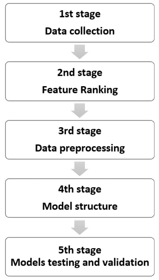
Figure 1.
Diagram of the methodology.
2.1. Data Collection
In this study, the actual data set employed was taken from 42 vertical wells. The data set contains surface pressure (SP), slurry flow rate (SFR), surface proppant concentration (SPC), tubing inside diameter (TID), pressure gauge depth (PGD), gel load (GL), proppant size (PZ), and proppant specific gravity (PSG). The models were constructed and validated using these data and were compared with the actual BHP measured by downhole pressure gauges. This research starts with the collection of data that has 485,442 data points from 42 vertical wells in the western desert of Egypt. The datasets contain the parameters listed in Table 1. All these wells were using borate cross-linked guar-based fracturing fluid. This fluid polymer is hydroxypropyl guar (HPG). Additionally, this study examined two types of proppant—high-strength proppant (HSP) and intermediate-strength proppant (ISP)—at different mesh sizes and specific gravities. The hydraulic fracturing treatment data set is quite diverse, including a broad range of hydraulic fracturing treatment parameters, proppant specifications, gel loads, and well completion parameters. Additionally, this approach not only provided flexibility to the model, but the model also became better able to cope with the challenges of such a wide range of parameters.

Table 1.
Statistical analysis for the collected database.
The pairwise relationships among the key variables in the dataset used to predict BHP are visualized with the pair plot in Figure 2. It is visualized with diagonal subplots showing the distribution of each variable and off-diagonal scatter plots denoting correlations between bivariate variables. Patterns of note are linear trends in variables, including SP, BHP, and SFR, indicating possible dependencies. Categorical data are sparse and discrete points in variables such as proppant size and proppant-specific gravity. These insights are essential for understanding the machine learning model’s operational parameters and optimization.
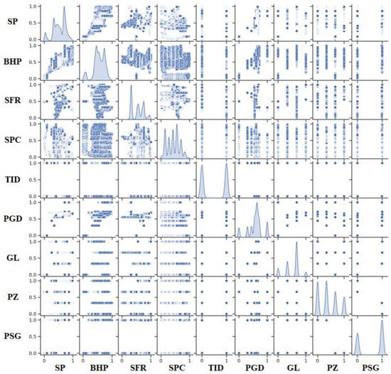
Figure 2.
Pair plot of the total data set used for BHP prediction.
The parameters used to predict BHP are shown in Figure 3, using violin plots. In the violin plot, we can see the distributions in multiple parameters along the x-axis, and on the y-axis, we see normalized values from 0 to 1. It combines box plots and kernel density estimates to give quick statistical summaries while obtaining insights into the underlying data distribution. Each violin represents the median as a central white line and a thicker black bar showing the interquartile range (IQR) around the middle 50% of the data. The width of the violin changes—the wider it is, the greater the data density is, and the narrower it is, the lower the data density is. Individual point displays are used for outliers rather than being integrated into the overall density profile. Significant differences exist between the distributions for all parameters. For instance, SP and BHP have symmetric and dense shapes (asymmetric lengths and widths), implying low variability and stable means. SFR has a narrow, peaked distribution, implying tightly clustered values. Visually, TID appears bimodal, displaying two distinct density peaks indicating two value clusters. The distribution of GL is broad, with more variable values. PZ also has a narrow, focused distribution that mimics a consistently measured response, as does the PSG distribution.
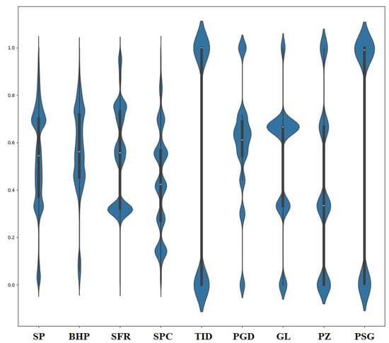
Figure 3.
Violin plots showing the distribution of key parameters for bottomhole pressure prediction. The horizontal axis represents input parameters, while the vertical axis shows their normalized values and variability.
2.2. Feature Ranking
Fundamental fluid mechanics guided us in selecting the features that would become the input to our machine learning model. BHP is primarily ruled by three main pressure components that include surface pressure alongside hydrostatic pressure and frictional pressure losses. The selection of input parameters involved the careful consideration of these basic factors, which provided a comprehensive representation. Other factors, such as temperature, Young’s modulus, leak-off coefficient, reservoir pressure, and in-situ stresses, can influence BHP; their effects are either indirectly captured by the chosen variables, such as surface pressure and pressure gauge depth measurements, or provide too many complexities to improve model accuracy significantly. Furthermore, additional parameters would increase all three noise factors, computational cost, and redundancy while possibly leading to overfitting without significant improvements to predictive abilities. Our strategy successfully selects features that maintain physical meaning and prediction precision to deliver accurate results in field applications. Our approach focuses on core governing factors to offer an efficient and robust BHP prediction method that prevents complexity-related issues and maintains solutions across different well conditions.
Data sets provide insights to ML models. These models are dependent on the caliber and interrelation of input features with the target variable. Consequently, the importance of features related to correlation coefficients is worth studying. Two different methodologies were used to calculate the correlation coefficient, for which Pearson’s and Spearman’s coefficients were used in this study. If two continuous variables are normally distributed, then Pearson’s correlation coefficient (r) measures that linear relationship, but it is sensitive to outliers. Spearman’s rank correlation coefficient (ρ), on the other hand, is more robust to outliers, suitable for ordinal, non-normally distributed data, and measures monotonic relationships with ranked data. Since Pearson’s r is best for testing for strict linear correlations and Spearman’s ρ for general increasing or decreasing trends, regardless of them being perfectly linear. The r and ρ lie between −1 and +1. If a variable increases in proportion, then the other also increases proportionally, and then the value of +1 would be a perfect positive correlation. If you were to have a perfect negative correlation, you would have one variable increasing while the other decreased in a perfectly predictable manner, and the value would be −1, and 0 means no correlation. Equations (6) and (7) show the formula for both criteria.
where:
- ▪
- Xi and Yi are the individual data points;
- ▪
- and are the means of X and Y;
- ▪
- The numerator is the covariance of X and Y;
- ▪
- The denominator is the product of their standard deviations.
- ▪
- di is the difference between the ranks of corresponding values in X and Y;
- ▪
- n is the number of data points.
Figure 4 provides a visual representation of the importance of input parameters to end BHP, like SP, SFR, SPC, TID, PGD, GL, PZ, and PSG. In particular, strong correlations exist between BHP and SP and PGD and SFR, while the remaining parameters display moderate correlations.
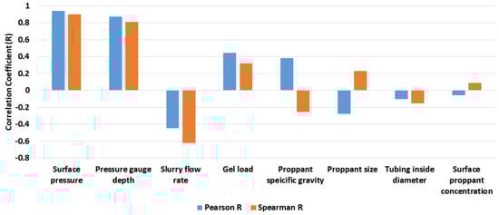
Figure 4.
Feature ranking of the input parameters with bottomhole pressure.
The heat map in Figure 5 depicts a visual form of the correlation matrix based on Pearson criteria for the BHP input parameters, which display the relationships between parameters. The heat map shows strong correlations among the parameters, with a near-perfect positive correlation for SP against BHP (0.94) and PGD against BHP (0.87), which is a strong interdependence. Parameters such as TID and PGD have weak correlations and thus appear relatively independent of other variables. These insights emphasize important parameter dependence and independence relationships that are key to understanding system dynamics and predicting their behavior.
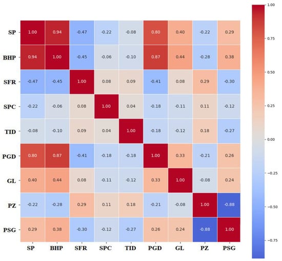
Figure 5.
Pearson’s correlation coefficient criteria are shown in the heat map of the total dataset used for the prediction of BHP.
The Spearman’s correlation coefficients between the features used to predict BHP in a data set are represented in the heatmap presented in Figure 6. SP and PGD are strongly positively correlated with BHP (0.90 and 0.96, respectively) and have a strong direct relationship with BHP. On the contrary, BHP shows a weak inverse relationship with SFR (−0.62). A minimally direct influence is deduced from other features that show weaker correlations with BHP, either positive or negative, namely SPC, TID, GL, PZ, and PSG.
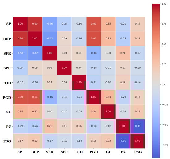
Figure 6.
Spearman’s correlation coefficient criteria are shown in the heat map of the total dataset used for the prediction of BHP.
2.3. Data Preprocessing
A thorough and intensive analysis was performed on the raw data to detect and remove the faulty entries in the dataset to generate complete historical data. By defining this via a systematic approach to data cleaning, we not only set a basis for the rest of the preprocessing stages, such as outlier detection, removal, and data integration and normalization procedures, but we also highlighted a set of steps that can be performed manually while minimizing the errors caused by human bias.
Normalization is a fundamental machine learning preprocessing step, standardizing features but not changing their value distributions. As a result, all features must conform to a uniform scale within the [0, 1] range and optimize model performance. More importantly, it will be particularly evident as algorithms become increasingly reliant on distance metrics or gradient-based optimization such as k-nearest neighbors, support vector machines (SVM), and neural networks. When normalization is not considered, features with larger numeric ranges can overwhelm model behavior, often at the expense of features of smaller range.
Normalization techniques demonstrate impressive benefits in a model’s training efficiency and effectiveness in their implementation. The optimization process converges faster with consistent gradient scales across features. It standardizes the problem so that the learning process is not prone to potential biases in the feature contribution to model development. Additionally, through normalization of proportionality relationships between features, model interpretability is improved, making it easier to analyze model behavior and decisions with greater precision.
Among the many normalization techniques, Min–Max scaling seems to be a robust way of standardizing features. This approach normalizes data so that they all squeeze into what is traditionally [0, 1] and preserves the order and metrics between data points. Specifically, Min–Max scaling is so useful for algorithms that need bounded input because it preserves these relationships, meaning Min–Max scaling is especially applicable to algorithms such as those using activation functions Sigmoid or Tanh.
The mathematical framework for Min–Max scaling can be expressed as follows:
where X is the input data, XNormalized is the output that has been normalized, XMinimum is the minimum value of the input data, and XMaximum is the maximum value of the input data.
2.4. Models Structure
Python 3.13.1 was used to create eleven machine learning (ML) models. Different techniques were used to design all these models, including linear, decision tree-based, ensemble, and instance-based models, and neural networks. We selected this set of methodologies to enhance the findings of the study and increase their generalizability. We list all the models in this section, followed by a short description of each model and their hyperparameters, as shown in Table 2. The ten trees produced with the RF model are illustrated in Figure 7, which is known as the representation of the Pythagorean forest. Each of the trees was built randomly, and all drawn as Pythagorean trees. Usually, the best tree is that which has the least branches and the brightest color, which means attributes rarely suffice to split the branches. First, the data were generated to create the trees through a regression tree, and then the nodes of the tree were colored according to standard deviation.
Table 2.
Summary of the ML models used.
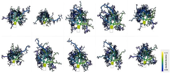
Figure 7.
Pythagorean forest shows all learned decision tree models from the RF model.
3. Results and Discussion
3.1. Model Results
Preprocessing was performed on the data set, and then training and testing sets were chosen from the data set. We split the data into two parts, an 80% training set and the remaining 20% as the test set. The performance metrics for the developed machine learning models are presented in Table 3 as mean square error (MSE), root mean square error (RMSE), mean absolute error (MAE), and coefficient of determination (R2). By computing these metrics, we get a thorough look at the accuracy as well as the explanatory power of each model.
Table 3.
Results of the developed ML models.
As shown in Figure 8, a gradient boosting model was compared against normalized actual BHP values obtained from pressure gauges downhole. The predicted BHP values are plotted on the horizontal axis, and the actual BHP measurements are plotted on the vertical axis. Normalized BHP ranges are shown in the color-coded regions and mapped from blue (low values) to yellow (high values) on the color bar to the right. The data points are very close to the diagonal line. This suggests that the gradient boosting model predicts BHP very well since the actual measurements we see are closely predicted. The model’s accuracy across different BHP ranges is further illustrated by the color gradient and clustering of points along the diagonal. The small scatter about the diagonal sees minor deviations from predictions to actual values, and they are not excessive and exhibit low bias. The evenness of colors along the line shows that the model has consistent information across the low (blue) to high (yellow) pressure range.
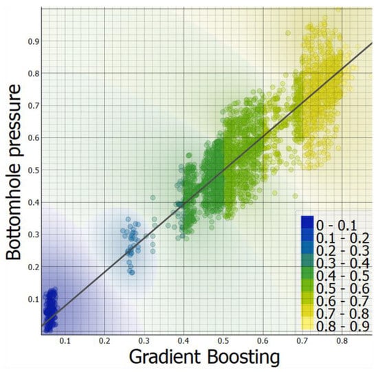
Figure 8.
Plots of normalized actual BHP versus predicted BHP by gradient boosting.
Figure 9 shows the principal variables affecting the BHP prediction using the gradient boosting model based on SHAP (SHapley Additive exPlanations) values. The SHAP values provide a quantitative description of each feature’s contribution to the model’s prediction and, hence, can be used to explain model behavior. On the horizontal axis are the SHAP values or the impact (positive or negative) of each parameter on the model output. Each data point represents a single observation in the data set and is colored by the value of the feature it belonged to (blue for the lowest and red for the highest) and positioned according to the given SHAP values between 0 and 1.
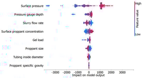
Figure 9.
SHAP plot of the gradient boosting model.
Parameters are ordered vertically and descending in importance, with the most influential parameter at the top. This case shows that SP is responsible for the most variation in BHP prediction and thus has the largest spread of SHAP values in both positive and negative directions. High SP values (red) usually lead to higher BHP, and low values (blue) lead to lower BHP. Other important parameters, including PGD and SFR, also show considerable ranges of SHAP values, indicating a considerable impact on BHP prediction. For these features, their color gradations denote the interaction between values in the low and high ends with their own effects.
Compared to the impact parameters, the less important ones, such as PSG and TID, have narrower ranges of SHAP values, so their influence on the model output is relatively minor. However, the visualization shows consistent trends wherein the contribution of certain values of these features is positive or negative for BHP predictions.
The gradient boosting model has been able to capture non-linear and complex interactions between input features and the BHP, as shown in this figure. SHAP values enable domain experts to interpret these same results, understand the model’s decision-making process, identify critical operational factors, and validate the physical meaning of the parameters used in the study.
3.2. Model Testing and Validation
The performance of the developed ML models is assessed with reference to the k-fold cross-validation testing in combination with random sampling methods. These approaches offer a structured methodology for checking the effectiveness of the models and a common approach for measuring their credibility and usefulness. Cross-validation is a kind of statistical method that is used to know, on a given dataset, how much the performance of a machine learning model will be capable of generalizing. It entails developing a number of subdivisions of the same dataset, which are referred to as the folds, and then one-fold is used in the model testing while the remainder is employed in the training process. This is carried out iteratively, especially when each of the data folds is used once to test the performance of the model. The model is assessed by averaging the corresponding scores obtained in each fold. The main purpose of cross-validation is to reduce the chance of overfitting, where a model performs well on the training data but badly on the test data. Cross-validation represents a more valid estimation of the model performance on new data where the data set is split into several independent test sets. It asserts that during the k-fold cross-validation procedure, the data set is partitioned into k subsets. In this model, k-1 folds are cross-validated for training, and the remaining one is used for testing the performance of the classification model. It is performed k times, and in each iteration, one-fold is used as a test set. The decision produced by the K-fold cross-validation process with K = 10 is reported in Table 4. The results for each model produce the corresponding MSE, RMSE, MAE, and R2.
Table 4.
Result of the K-fold cross-validation procedure.
Repeated random sampling involves partitioning the data set into training and test sets in a fixed ratio and performing this process several times. The relevance of this method is in the fact that splitting the data several times provides a better estimate of the performance measures since the measures calculated from a single split of the data may be rather variable. To offset the problem of data splitting, the average performance of the model from many experiments is obtained so that the model’s generality can be assessed. Table 5 shows the results of the repeated random sampling technique in which a total of 10 iterations were performed. All the models are presented with their MSE, RMSE, MAE, and R2 values.
Table 5.
Result of random sampling procedure.
3.3. Field Application
The oil well, well X, is located in the western desert of Egypt. The well was drilled to 8500 feet. Formation Y is a conventional sandstone reservoir, and the optimum method for enhancing the productivity index was to implement the hydraulic fracturing treatment. Table 6 and Figure 10 present the input data for each parameter.
Table 6.
Well-X input parameters.
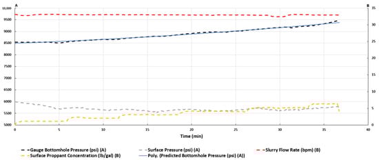
Figure 10.
Real-time monitoring of hydraulic fracturing treatment in well A.
The developed gradient boosting model, the most accurate algorithm, has been run with the data from well X to forecast the real-time BHP during fracturing treatment. The comparison between the BHP predicted by the developed gradient boosting algorithm and the BHP measured by the memory gauge is shown in Figure 10. It can easily be perceived that the model’s predictions are accurate. In this situation, this should enable continuous real-time monitoring of hydraulic fracturing treatment performance and allow for a rapid reaction to the optimizing decision while pumping.
Well X demonstrates successful field use of the gradient boosting model to estimate real-time BHP during fracturing for individual wells with high accuracy. This represents a breakthrough that not only enables real-time monitoring and optimization of hydraulic fracturing treatments but also offers an effective alternative to expensive and time-consuming deployed bottomhole pressure gauges and inaccurate physics-based models, empirical correlations, and hybrids. This actual application proves that advancement in predictive modeling is essential to improve operational efficiency and to progress the decision-making process in petroleum engineering, especially in complex reservoir environments.
3.4. Limitations and Future Perspectives
Multiple limitations exist regarding the application of our developed ML model that predicts real-time BHP in hydraulic fracturing operations. The model training used a data set containing multiple operational and completion conditions of 42 vertical wells, yet its ability to predict outside these established operational and completion conditions demands further assessment. In addition, real-time BHP predictions made using this model depend on accurate historical data because sensor measurement errors and fast pressure changes can lead to prediction inaccuracies. Additionally, ML struggles with delivering direct interpretations of results since its approaches lack the mathematical foundations that physics-based models possess. The future development of ML should target the creation of physics-informed algorithms that merge fluid mechanics principles with data-driven learning methods to enhance prediction stability. A broader wells data set, including various inputs, such as inclination angle, SP, SFR, SPC, TID, PGD, GL, PZ, and PSG, will boost the model’s adaptability. The testing of the developed models with real bottomhole pressure gauges under different operational conditions must be performed accurately to prove their reliability when used in dynamic fracturing systems. By addressing these limitations, future studies can further refine ML-physics hybrid models, leading to more accurate, interpretable, and field-deployable solutions for real-time BHP estimation in hydraulic fracturing operations.
4. Conclusions
This study has demonstrated the feasibility of predicting the bottomhole pressure during fracturing using machine learning and deep learning algorithms. These results further emphasize the power of a holistic approach in which the combination of different ML models leads to a dramatic increase in prediction accuracy. The applicability and reliability of the model were expanded using a comprehensive dataset from 42 vertical wells containing fluid, proppant, and completion, as well as operational parameters. Statistical analysis demonstrates critical relationships between bottomhole pressure, surface pressure, and gauge depth, indicating the significant impact of hydrostatic and friction pressure. Feature ranking identified slurry flow rate, surface pressure, and gauge depth as key factors for bottomhole pressure prediction, which gives hydraulic fracturing engineers the insight to improve treatment designs and prevent premature proppant screenouts.
Data quality issues and feature dominance were addressed by rigorous data preprocessing, specifically Min–Max normalization, leading to the best possible model performance. We evaluated simple ML models, such as linear regression and stochastic gradient descent models, against more advanced ML models, such as gradient boosting and neural networks, and found that these more advanced models could outperform simple models with high accuracy for capturing complex physical interactions. A high correlation coefficient (R2 = 0.931) and very low mean square error (MSE = 0.003), achieved through k-fold cross-validation and repeated random sampling, verified the developed model. Additionally, well X successfully used the gradient boosting model to predict real-time bottomhole pressure, demonstrating a data-driven, low-cost alternative to expensive bottomhole pressure gauges and inaccurate traditional calculation methods.
This work provides a comprehensive framework for leveraging ML to predict bottomhole pressure with high precision and establish its capability to revolutionize hydraulic fracturing optimization. This study also succeeded in quantifying the impact of algorithm selection on prediction accuracy and thereby lays the foundation for improved decision-making during hydraulic fracturing and, ultimately, for enhanced efficiency and reduced cost in complex reservoir environments.
Author Contributions
Conceptualization, S.N.; methodology, R.M.; validation, S.N.; formal analysis, S.N.; investigation, S.N.; resources, R.M.; data curation, R.M.; writing—original draft preparation, S.N.; writing—review and editing, R.M.; visualization, S.N.; supervision, R.M.; project administration, R.M. All authors have read and agreed to the published version of the manuscript.
Funding
This research received no external funding.
Data Availability Statement
The original contributions presented in the study are included in the article, further inquiries can be directed to the corresponding authors.
Conflicts of Interest
The authors declare no conflicts of interest.
Nomenclature
| Cv | Volume Fraction Solids in Slurry |
| d | Pipe inside diameter, inches |
| FD | Pipe friction cross-link delay factor, dimensionless |
| FF | Pipe friction correction factor, dimensionless |
| FS | Friction factor for solids addition, dimensionless |
| k′ | Fluid consistency index, lb-secn/ft2 |
| L | Pipe length, feet |
| n′ | Power-law exponent, dimensionless |
| P | Pressure, psia |
| P1 | Friction pressure term in laminar flow, dimensionless |
| ΔP | Friction pressure drop, psi |
| Q | Pump rate, bpm |
| Ret | Reynold’s number at transition to turbulent flow, dimensionless |
| ρF | Fluid density, g/cm3 |
| ρ | Spearman’s rank correlation coefficient |
| t | Time, minutes |
| Tf | Coefficient for turbulent flow friction pressure drop, dimensionless |
| TF | Temperature, degrees Fahrenheit |
| Xs | Increase in friction with solids addition, dimensionless |
| Adam | Adaptive Moment Estimation optimization algorithm |
| DT | Decision Trees |
| GB | Gradient Boosting |
| kNN | K-Nearest Neighbor |
| L-BFGS | Limited-memory-Broyden-Fletcher-Goldfarb-Shanno optimization algorithm |
| LR | Linear Regression |
| MAE | Mean absolute error |
| MAPE | Mean absolute percent error |
| ML | Machine learning |
| MSE | Mean square error |
| NN | Neural Network |
| R2 | Correlation coefficients |
| r | Pearson’s correlation coefficient |
| RF | Random Forest |
| RMSE | Root mean square error |
| SGD | Stochastic Gradient Descent |
| SHAP | SHapley Additive exPlanations |
| SVM | Support Vector Machines |
| SP | Surface pressure |
| BHP | Bottomhole pressure |
| SFR | Slurry flow rate |
| SPC | Surface proppant concentration |
| TID | Tubing inside diameter |
| PGD | Pressure gauge depth |
| GL | Gel load |
| PZ | Proppant size |
| PSG | Proppant Speicific Gravity |
References
- Li, Q.; Li, Q.; Cao, H.; Wu, J.; Wang, F.; Wang, Y. The Crack Propagation Behaviour of CO2 Fracturing Fluid in Unconventional Low Permeability Reservoirs: Factor Analysis and Mechanism Revelation. Processes 2025, 13, 159. [Google Scholar] [CrossRef]
- Li, Q.; Zhang, C.; Yang, Y.; Ansari, U.; Han, Y.; Li, X.; Cheng, Y. Preliminary experimental investigation on long-term fracture conductivity for evaluating the feasibility and efficiency of fracturing operation in offshore hydrate-bearing sediments. Ocean Eng. 2023, 281, 114949. [Google Scholar] [CrossRef]
- Nizamidin, N.; Kim, A.; Belcourt, K.; Angeles, M.; Kim, D.H.; Matovic, G.; Lege, E. New Casing Friction Model for Slickwater: Field Data Validation, Application, and Optimization for Hydraulic Fracturing. In Proceedings of the SPE Hydraulic Fracturing Technology Conference and Exhibition, January 2022; OnePetro: Richardson, TX, USA, 2022. [Google Scholar] [CrossRef]
- Jannise, R.C.; Edwards, W.J. Innovative Method for Predicting Downhole Pressures During Frac-Pack Pumping Operations Facilitates More Successful Completions. In Proceedings of the Asia Pacific Oil and Gas Conference and Exhibition, October 2007; OnePetro: Richardson, TX, USA, 2007. [Google Scholar] [CrossRef]
- Kim, G.-H.; Wang, J.Y. Interpretation of Hydraulic Fracturing Pressure in Low-Permeability Gas Formations. In Proceedings of the SPE Production and Operations Symposium, March 2011; OnePetro: Richardson, TX, USA, 2011. [Google Scholar] [CrossRef]
- Shaoul, J.R.; Folmar, E.; Arman, J.V.; van Gijtenbeek, K. Real-Data Analysis Brings Large Benefits in Hydraulic Fracturing in a Moderate Permeability Oil Reservoir in Kazakhstan. In Proceedings of the SPE Western Regional/AAPG Pacific Section Joint Meeting, May 2002; OnePetro: Richardson, TX, USA, 2002. [Google Scholar] [CrossRef]
- Tinker, S.J.; Baycroft, P.D.; Ellis, R.C.; Fitzhugh, E. Mini-Frac Tests and Bottomhole Treating Pressure Analysis Improve Design and Execution of Fracture Stimulations. In Proceedings of the SPE Production Operations Symposium, March 1997; OnePetro: Richardson, TX, USA, 1997. [Google Scholar] [CrossRef]
- Tan, H.C.; Wesselowski, K.S.; Willingham, J.D. Delayed Borate Crosslinked Fluids Minimize Pipe Friction Pressure. In Proceedings of the SPE Rocky Mountain Regional Meeting, May 1992; OnePetro: Richardson, TX, USA, 1992. [Google Scholar] [CrossRef]
- Downie, R.C.; Fagan, R.E. Proppant Effects on Fracturing Fluid Friction. In Proceedings of the SPE Mid-Continent Gas Symposium, May 1994; OnePetro: Richardson, TX, USA, 1994. [Google Scholar] [CrossRef]
- Wright, T.B.; Aud, W.W.; Cipolla, C.; Meehan, D.N.; Perry, K.F.; Cleary, M.P. Identification and Comparison of True Net Fracturing Pressures Generated by Pumping Fluids with Different Rheology into the Same Formations. In Proceedings of the SPE Gas Technology Symposium, June 1993; OnePetro: Richardson, TX, USA, 1993. [Google Scholar] [CrossRef]
- Martinez, D.; Wright, C.A.; Wright, T.B. Field Application of Real-Time Hydraulic Fracturing Analysis. In Proceedings of the Low Permeability Reservoirs Symposium, April 1993; OnePetro: Richardson, TX, USA, 1993. [Google Scholar] [CrossRef]
- Bilden, D.M.; Spearman, J.W.; Hudson, H.G. Analysis of Observed Friction Pressures Recorded While Fracturing in Highly Deviated Wellbores. In Proceedings of the SPE Production Operations Symposium, March 1993; OnePetro: Richardson, TX, USA, 1993. [Google Scholar] [CrossRef]
- Xu, Z.; Wu, K.; Song, X.; Li, G.; Zhu, Z.; Pang, Z. A Unified Model to Predict Flowing Pressure and Temperature Distributions in Horizontal Wellbores for Different Energized Fracturing Fluids. In Proceedings of the SPE/AAPG/SEG Unconventional Resources Technology Conference, July 2018; OnePetro: Richardson, TX, USA, 2018. [Google Scholar] [CrossRef]
- Ye, J.; Do, N.C.; Zeng, W.; Lambert, M. Physics-informed neural networks for hydraulic transient analysis in pipeline systems. Water Res. 2022, 221, 118828. [Google Scholar] [CrossRef] [PubMed]
- Shah, S.; Zhou, Y.; Bailey, M.; Hernandez, J. Correlations to Predict Frictional Pressure of Hydraulic Fracturing Slurry in Coiled Tubing. In Proceedings of the International Oil & Gas Conference and Exhibition in China, December 2006; OnePetro: Richardson, TX, USA, 2006. [Google Scholar] [CrossRef]
- Abdulwarith, A.; Ammar, M.; Kakadjian, S.; McLaughlin, N.; Dindoruk, B. A Hybrid Physics Augmented Predictive Model for Friction Pressure Loss in Hydraulic Fracturing Process Based on Experimental and Field Data. In Proceedings of the Offshore Technology Conference, April 2024; OnePetro: Richardson, TX, USA, 2024. [Google Scholar] [CrossRef]
- Barree, R.D.; Gilbert, J.V.; Conway, M.W. An Effective Model for Pipe Friction Estimation in Hydraulic Fracturing Treatments. In Proceedings of the SPE Rocky Mountain Petroleum Technology Conference, April 2009; OnePetro: Richardson, TX, USA, 2009. [Google Scholar] [CrossRef]
- Zhou, J.; Sun, H.; Stevens, R.; Qu, Q.; Bai, B. Bridging the Gap between Laboratory Characterization and Field Applications of Friction Reducers. In Proceedings of the SPE Production and Operations Symposium, March 2011; OnePetro: Richardson, TX, USA, 2011. [Google Scholar] [CrossRef]
- Mack, D.J.; Baumgartner, S.A. Friction Pressure of Foamed Stimulation Fluids Evaluated With an On-Site Computer. In Proceedings of the SPE Annual Technical Conference and Exhibition, October 1986; OnePetro: Richardson, TX, USA, 1986. [Google Scholar] [CrossRef]
- Muravyova, E.A.; Enikeeva, E.R.; Alaeva, N.N. Application of Bottom Hole Pressure Calculation Method for the Management of Oil Producing Well. In Proceedings of the 2020 International Multi-Conference on Industrial Engineering and Modern Technologies (FarEastCon), Vladivostok, Russia, 6–9 October 2020; pp. 1–5. [Google Scholar] [CrossRef]
- Aziz, K. Calculation of Bottom-Hole Pressure in Gas Wells. J. Pet. Technol. 1967, 19, 897–899. [Google Scholar] [CrossRef]
- Hannah, R.R.; Harrington, L.J.; Lance, L.C. The Real-Time Calculation of Accurate Bottomhole Fracturing Pressure From Surface Measurements Using Measured Pressures as a Base. In Proceedings of the SPE Annual Technical Conference and Exhibition, October 1983; OnePetro: Richardson, TX, USA, 1983. [Google Scholar] [CrossRef]
- El-Saghier, R.M.; El Ela, M.A.; El-Banbi, A. A model for calculating bottom-hole pressure from simple surface data in pumped wells. J. Pet. Explor. Prod. Technol. 2020, 10, 2069–2077. [Google Scholar] [CrossRef]
- Tan, H.C.; Shah, S. Field Application of Laboratory Friction Pressure Correlations for Borate Crosslinked Fluids. In Proceedings of the SPE International Symposium on Oilfield Chemistry, February 1991; OnePetro: Richardson, TX, USA, 1991. [Google Scholar] [CrossRef]
- Malkin, A.Y.; Derkach, S.R.; Kulichikhin, V.G. Rheology of Gels and Yielding Liquids. Gels 2023, 9, 715. [Google Scholar] [CrossRef] [PubMed]
- Maxian, O.; Peláez, R.P.; Mogilner, A.; Donev, A. Simulations of dynamically cross-linked actin networks: Morphology, rheology, and hydrodynamic interactions. PLOS Comput. Biol. 2021, 17, e1009240. [Google Scholar] [CrossRef]
- Zhou, H.; Guo, J.; Zhang, T.; Zeng, J. Friction characteristics of proppant suspension and pack during slickwater hydraulic fracturing. Geoenergy Sci. Eng. 2023, 222, 211435. [Google Scholar] [CrossRef]
- Anschutz, D.; Wildt, P.; McGill, M.; Lowrey, T.; Contreras, K. Understanding the Shear History of Various Loadings of Friction Reducers and the Associated Impact on the Fluid’s Stability, Pipe Friction Reduction, and Effect on Proppant Transport and Deposition in Both Fresh Water and Brine Base Fluid. In Proceedings of the SPE Hydraulic Fracturing Technology Conference and Exhibition, January 2023; OnePetro: Richardson, TX, USA, 2023. [Google Scholar] [CrossRef]
- Pandey, V.J.; Robert, J.A. New Correlation for Predicting Frictional Pressure Drop of Proppant-Laden Slurries Using Surface Pressure Data. In Proceedings of the International Symposium and Exhibition on Formation Damage Control, February 2002; OnePetro: Richardson, TX, USA, 2002. [Google Scholar] [CrossRef]
- Guo, Y.; Zhang, M.; Yang, H.; Wang, D.; Ramos, M.A.; Hu, T.S.; Xu, Q. Friction Challenge in Hydraulic Fracturing. Lubricants 2022, 10, 14. [Google Scholar] [CrossRef]
- Al Balushi, F.; Zhang, Q.; Taleghani, A.D. On the impact of proppants shape, size distribution, and friction on adaptive fracture conductivity in EGS. Geoenergy Sci. Eng. 2024, 241, 213115. [Google Scholar] [CrossRef]
- Ramlan, A.S.; Zin, R.M.; Bakar, N.F.A.; Othman, N.H. Recent progress on proppant laboratory testing method: Characterisation, conductivity, transportation, and erosivity. J. Pet. Sci. Eng. 2021, 205, 108871. [Google Scholar] [CrossRef]
- Terminiello; Nasca, M.; Filipich, J.; Intyre, D.M.; Crespo, P. From WHP to BHP Using Machine Learning in Multi-Fractured Horizontal Wells of the Vaca Muerta Formation. In Proceedings of the SPE/AAPG/SEG Unconventional Resources Technology Conference, June 2022; OnePetro: Richardson, TX, USA, 2022. [Google Scholar] [CrossRef]
- Dunham, E.M.; Zhang, J.; Moos, D. Constraints on Pipe Friction and Perforation Cluster Efficiency from Water Hammer Analysis. In Proceedings of the SPE Hydraulic Fracturing Technology Conference and Exhibition, January 2023; OnePetro: Richardson, TX, USA, 2023. [Google Scholar] [CrossRef]
- Ishak, K.E.H.K.; Khan, J.A.; Padmanabhan, E.; Ramalan, N.H.M. Friction reducers in hydraulic fracturing fluid systems—A review. AIP Conf. Proc. 2023, 2682, 030004. [Google Scholar] [CrossRef]
- Keck, R.G.; Reiter, D.F.; Lynch, K.W.; Upchurch, E.R. Analysis of Measured Bottomhole Treating Pressures During Fracturing: Do Not Believe Those Calculated Bottomhole Pressures. In Proceedings of the SPE Annual Technical Conference and Exhibition, October 2000; OnePetro: Richardson, TX, USA, 2000. [Google Scholar] [CrossRef]
- Li, N.-L.; Chen, B. Evaluation of frictional pressure drop correlations for air-water and air-oil two-phase flow in pipeline-riser system. Pet. Sci. 2024, 21, 1305–1319. [Google Scholar] [CrossRef]
- Fragachan, F.E.; Mack, M.G.; Nolte, K.G.; Teggin, D.E. Fracture Characterization From Measured and Simulated Bottom hole Pressure. In Proceedings of the Low Permeability Reservoirs Symposium, April 1993; OnePetro: Richardson, TX, USA, 1993. [Google Scholar] [CrossRef]
- Shah, S.N.; Lord, D.L.; Tan, H.C. Recent Advances in the Fluid Mechanics and Rheology of Fracturing Fluids. In Proceedings of the International Meeting on Petroleum Engineering, March 1992; OnePetro: Richardson, TX, USA, 1992. [Google Scholar] [CrossRef]
- Shah, S.N.; Harris, P.C.; Tan, H.C. Rheological Characterization of Borate Crosslinked Fracturing Fluids Employing a Simulated Field Procedure. In Proceedings of the SPE Production Technology Symposium, November 1988; OnePetro: Richardson, TX, USA, 1988. [Google Scholar] [CrossRef]
- Sircar, A.; Yadav, K.; Rayavarapu, K.; Bist, N.; Oza, H. Application of machine learning and artificial intelligence in oil and gas industry. Pet. Res. 2021, 6, 379–391. [Google Scholar] [CrossRef]
- Tariq, Z.; Aljawad, M.S.; Hasan, A.; Murtaza, M.; Mohammed, E.; El-Husseiny, A.; Alarifi, S.A.; Mahmoud, M.; Abdulraheem, A. A systematic review of data science and machine learning applications to the oil and gas industry. J. Pet. Explor. Prod. Technol. 2021, 11, 4339–4374. [Google Scholar] [CrossRef]
- Gabry, M.A.; Ali, A.G.; Elsawy, M.S. Application of Machine Learning Model for Estimating the Geomechanical Rock Properties Using Conventional Well Logging Data. In Proceedings of the Offshore Technology Conference, April 2023; OnePetro: Richardson, TX, USA, 2023. [Google Scholar] [CrossRef]
- Gharieb, A.; Adel Gabry, M.; Algarhy, A.; Elsawy, M.; Darraj, N.; Adel, S.; Taha, M.; Hesham, A. Revealing Insights in Evaluating Tight Carbonate Reservoirs: Significant Discoveries via Statistical Modeling. An In-Depth Analysis Using Integrated Machine Learning Strategies. In Proceedings of the GOTECH, May 2024; OnePetro: Richardson, TX, USA, 2024. [Google Scholar] [CrossRef]
- Saihood, T.; Samuel, R. Mud Loss Prediction in Realtime Through Hydromechanical Efficiency. In Proceedings of the ADIPEC, October 2022; OnePetro: Richardson, TX, USA, 2022. [Google Scholar] [CrossRef]
- Sahood, T.; Myers, M.T.; Hathon, L.; Unomah, G.C. Quantifying the Mechanical Specific Energy (MSE) with Differential Wellbore Pressure for Real-Time Well Automation. In Proceedings of the Offshore Technology Conference, April 2024; OnePetro: Richardson, TX, USA, 2024. [Google Scholar] [CrossRef]
- Thabet, S.; Elhadidy, A.; Elshielh, M.; Taman, A.; Helmy, A.; Elnaggar, H.; Yehia, T. Machine Learning Models to Predict Total Skin Factor in Perforated Wells. In Proceedings of the SPE Western Regional Meeting, April 2024; OnePetro: Richardson, TX, USA, 2024. [Google Scholar] [CrossRef]
- Gharieb, A.; Gabry, M.A.; Elsawy, M.; Algarhy, A.; Ibrahim, A.F.; Darraj, N.; Sarker, M.R.; Adel, S. Data Analytics and Machine Learning Application for Reservoir Potential Prediction in Vuggy Carbonate Reservoirs Using Conventional Well Logging. In Proceedings of the SPE Western Regional Meeting, April 2024; OnePetro: Richardson, TX, USA, 2024. [Google Scholar] [CrossRef]
- Thabet, S.; Zidan, H.; Elhadidy, A.; Taman, A.; Helmy, A.; Elnaggar, H.; Yehia, T. Machine Learning Models to Predict Production Rate of Sucker Rod Pump Wells. In Proceedings of the SPE Western Regional Meeting, April 2024; OnePetro: Richardson, TX, USA, 2024. [Google Scholar] [CrossRef]
- Saihood, T.; Saihood, A.; Al-Shaher, M.A.; Ehlig-Economides, C.; Zargar, Z. Fast Evaluation of Reservoir Connectivity via a New Deep Learning Approach: Attention-Based Graph Neural Network for Fusion Model. In Proceedings of the SPE Annual Technical Conference and Exhibition, September 2024; OnePetro: Richardson, TX, USA, 2024. [Google Scholar] [CrossRef]
- Thabet, S.A.; El-Hadydy, A.A.; Gabry, M.A. Machine Learning Models to Predict Pressure at a Coiled Tubing Nozzle’s Outlet During Nitrogen Lifting. In Proceedings of the SPE/ICoTA Well Intervention Conference and Exhibition, March 2024; OnePetro: Richardson, TX, USA, 2024. [Google Scholar] [CrossRef]
- Ben, Y.; Perrotte, M.; Ezzatabadipour, M.; Ali, I.; Sankaran, S.; Harlin, C.; Cao, D. Real-Time Hydraulic Fracturing Pressure Prediction with Machine Learning. In Proceedings of the SPE Hydraulic Fracturing Technology Conference and Exhibition, January 2020; OnePetro: Richardson, TX, USA, 2020. [Google Scholar] [CrossRef]
- Reznikov; Abdrazakov, D.; Chuprakov, D. Model-based interpretation of bottomhole pressure records during matrix treatments in layered formations. Pet. Sci. 2024, 21, 3587–3611. [Google Scholar] [CrossRef]
- Gabry, M.A.; Thabet, S.A.; Abdelhaliem, E.; Algarhy, A.; Palanivel, M. Ability to Use DFIT to Replace the Minifrac in Sandstone Formations for Reservoir Characterizations. In Proceedings of the SPE 2020 Symposium Compilation, January 2021; OnePetro: Richardson, TX, USA, 2021. [Google Scholar] [CrossRef]
Disclaimer/Publisher’s Note: The statements, opinions and data contained in all publications are solely those of the individual author(s) and contributor(s) and not of MDPI and/or the editor(s). MDPI and/or the editor(s) disclaim responsibility for any injury to people or property resulting from any ideas, methods, instructions or products referred to in the content. |
© 2025 by the authors. Licensee MDPI, Basel, Switzerland. This article is an open access article distributed under the terms and conditions of the Creative Commons Attribution (CC BY) license (https://creativecommons.org/licenses/by/4.0/).