Evaluation of Simulations for Short-Term Voltage Stability Assessment with Respect to Model Uncertainties

Abstract

In order to evaluate the short-term voltage stability of an electrical power grid, it is necessary to employ not only systematic and well-targeted fault simulations, but also an evaluation method that assesses the criticality of the individual scenarios. A binary decision between stable or unstable, or whether a threshold value is exceeded or not, is inadequate, particularly in instances where the modeling of the system is subject to a certain degree of uncertainty. Since systematic deviations are subject to natural principles and an intervention limit can thus be determined deterministically, an evaluation method is therefore required that allows a statement to be made about the proximity to instability or to a threshold value. It is common practice to employ indices for the evaluation of voltage recovery following a fault event in simulations or from real measurements. However, depending on the specific question being analyzed, the requirements for an index may vary. A review of the literature revealed the existence of several indices that have been developed and applied in the context of various problems and analyses. These indices have been shown to be effective in the respective contexts. However, none of them fully satisfy the requisite criteria for addressing the aforementioned issue. This paper presents and discusses a new index that was developed explicitly for the problem at hand in dealing with model uncertainties, derived requirements from it, and compared it with existing indices from the literature. The benefits of this novel index in comparison with the established ones were visualized based on a number of indicative simulations. Subsequently, the uncertainties inherent in the load parameterization and their implications on the voltage recovery were presented via Monte Carlo simulations. The evaluations of these effects in terms of the distance from the permissible threshold value were then analyzed using the various indices. All simulations were executed within the framework of the IEEE 39 bus New England system.

1. Introduction

The term short-term voltage stability refers to the ability of an electrical power system to return to a steady and permissible state after a severe disturbance with a massive voltage dip. In simulation studies, this is typically assumed to be a three-phase short circuit with a fault clearing time of 150 ms—according to the most severe failure type and maximum fault clearing time for instantaneous tripping. The evaluation is carried out based on dynamic simulations, which cover a time range of a few seconds. Nevertheless, this method of fault simulation can also identify issues pertaining to transient rotor angle stability. Consequently, investigations have frequently examined both phenomena concurrently [1,2].

In grid planning, various questions regarding short-term voltage stability can be addressed and analyzed using dynamic simulations. In order to recognize the need for intervention, the stability of the network must be constantly reviewed, taking into account new developments and forecasts, which requires close monitoring (e.g., [1]). In this context, the identification of critical grid regions can also play an important role [3]. Another aspect is the improvement in stability itself, for example, through the optimal installation of dynamic VAR compensation devices [4,5,6]. Other examples include the testing of operating strategies such as load shedding [3] or the improvement in voltage support from distributed generation units [7]. All of these analyses are characterized by a high number of necessary simulations, in which the voltage recovery at different measuring points must be evaluated. In practice, indices are frequently utilized for these purposes [3,4,5,6,7].

Several indices are presented in the literature [8,9], the suitability of which for the specific application depends on the respective question of the analysis. For example, the indices can provide a binary statement on

• whether a threshold value has been exceeded or
• whether a stable operating point has been reached again
• as well as qualitative statements, for example, about
• how strong voltage deviations are,
• how long a threshold value is exceeded, or
• how strong oscillations are.

The indices usually evaluate several of these qualitative aspects. This is carried out, for example, by means of sub-indices [3,4], which are combined into one index using weightings, or by calculating the integrals over time [5,6].

More recent metrics are increasingly based on the threshold values for permissible voltage recovery, as these can directly reflect the requirements from grid codes or the low-voltage ride-through (LVRT) capability of power-generating systems [5,6,7]. In this sense, the term ’stability’ should also be extended in this paper to include compliance with such threshold values.

To reliably predict the stability of a real power system, the correct modeling of components with fast dynamics is essential. Particular attention is often paid to the behavior of induction motors in loads, which are slowed down by voltage dips and exhibit a high reactive power draw when the voltage is restored due to the restart. This can lead to a fault-induced delayed voltage recovery (FIDVR) or, in the worst case, to a voltage collapse and rotor angle instability [2,8,10]. However, uncertainty in load modeling with regard to the stationary behavior (e.g., the shares in types of a ZIP-load) and dynamics are generally high, and therefore a critical aspect in the evaluation of simulation results.

When planning electrical networks, it is standard practice to assume the worst-case scenario, thus adopting a risk-averse approach. However, a problem arises when the number of parameters is excessively high, especially for dynamic load models [11], and estimating the worst-case scenario is both individual and challenging. Additionally, realistic parameterization is complicated by the high variability of loads [12]. In the context of the stability evaluation of real grids, additional challenges arise due to the large number of network use cases, potential fault locations, and the comparatively long calculation times for dynamic grid simulations.

It is therefore apparent that a metric is required to assist in the pre-selection of critical situations, and that can be applied effectively in contexts involving uncertainties. A purely qualitative statement about the stability is generally not sufficient to adequately evaluate the stability of a grid. Rather, it should be possible to distinguish between situations that are considered to be reliably stable and those that are close to threshold. The latter should be treated with a certain degree of caution. This applies, in particular, where threshold values also take into account the model limits, such as protective tripping, cascading phenomena, and the dynamic load behavior, which may not or may inadequately be modeled in the underlying models.

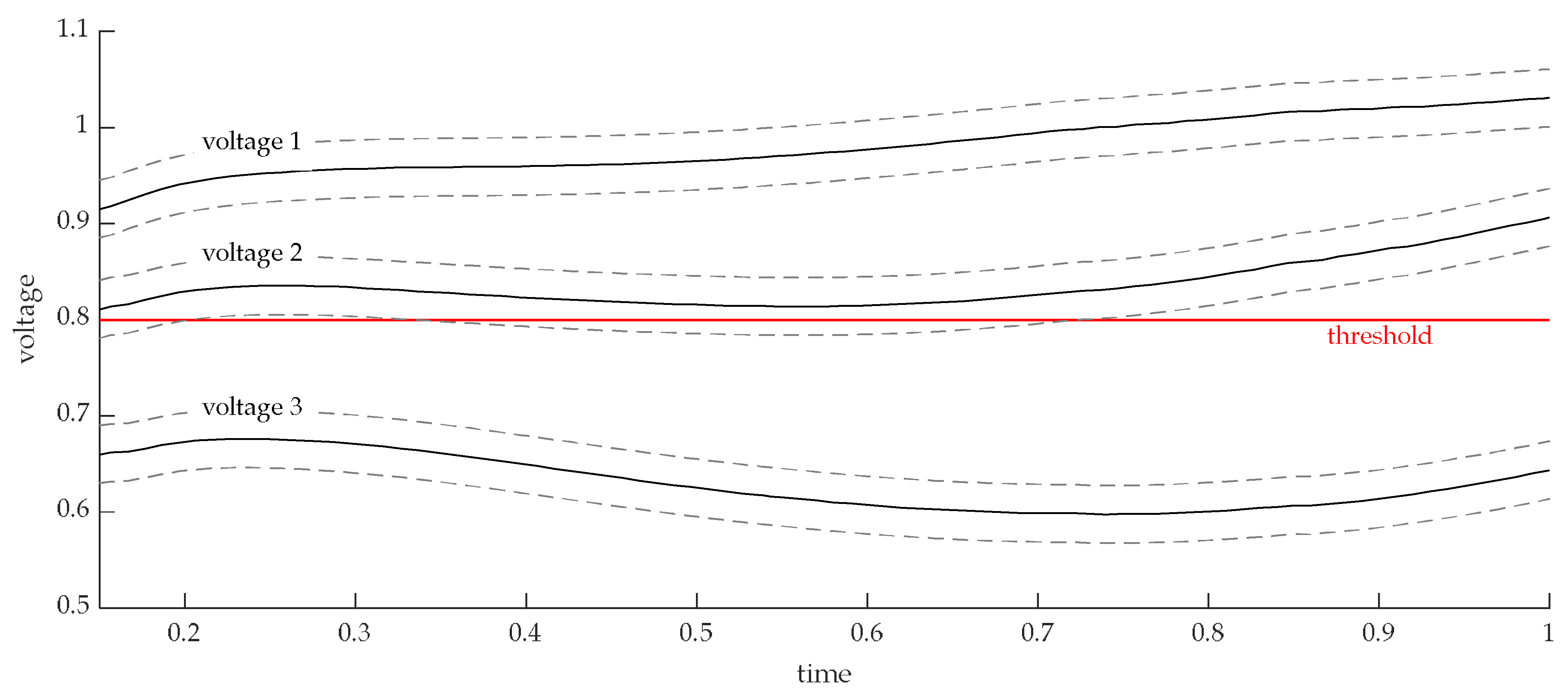
Figure 1 shows three exemplary voltage recovery curves after a fault event and a threshold value to be complied with. According to [13], when the uncertainties in the parameters are taken into account, the possible voltage curves can be represented as envelope curves around the calculated voltage curve with the initial parameters. These are shown as dashed lines in Figure 1 and thus symbolize the possible range of voltage recovery. It is obvious that voltage 3 was not permissible because it was completely below the threshold value. Voltages 1 and 2 were above the threshold value and could therefore be recognized as permissible. However, the envelope curve of voltage 2 exceeded the threshold value, which is why it could not be clearly classified as permissible due to the uncertainties. In contrast, voltage 1 was a great distance from the threshold value and could be assessed as permissible despite the uncertainties. In order to differentiate between borderline situations (voltage 2) and clearly permissible situations (voltage 1) and to avoid unnecessary additional simulations, a metric is needed that allows a statement to be made about the distance between the voltage and threshold curve. In other words, it should allow for gradation within the permissible voltage range in order to assess the distance to instability and to qualitatively distinguish between different events within the permissible voltage range.

In line with the problem discussed here, the we defined the following requirements for an index:

• Consideration of a gradation within the permissible voltage range to assess the distance to instability and qualitative distinctions between different events within the permissible voltage range;
• Binary statement option regarding the voltage behavior (i.e., a clear statement as to whether a threshold value has been exceeded or not);
• Standardization of the index for the purpose of simple interpretation and comparability between different grid usage cases and networks;
• Flexibility in setting the threshold values (e.g., to meet different grid code requirements). It should also be possible to represent the threshold value as a time-dependent function and to take both the upper and lower threshold values into account;
• Simple implementation: Calculations should be carried out exclusively from time series data, there should be no need for preliminary analyses, and calculations should be kept simple and computationally efficient;
• Flexible display: A temporal resolution per bus should be possible, but it should also be possible to calculate an index value per region and per network.

The following section will examine the indices that are available in the literature in order to ascertain their suitability in meeting the aforementioned requirements. It will be demonstrated that none of the aforementioned indices fully satisfy the requirements, thus necessitating the proposal of a new index in Section 3. This index will be tested in Section 4 and Section 5 using a number of exemplary simulations and compared with other indices. The purpose of these simulations is to illustrate that the new index’s capacity to capture gradation is a particular advantage in the present context.

2. Comparison of Indices from the Literature with Regard to the Requirements

A considerable number of indices exist within the scientific literature that evaluate the short-term voltage stability. The most significant of these indices, which are based on time series data, are presented below:

The Lyapunov exponent (LE) is founded upon the principles of ergodic theory and serves to quantify the degree of chaos inherent within a given system. This allows a binary statement about the stability of a system in terms of its ability to return to a steady state. The calculation necessitates a meticulous calibration of the index parameterization, which can prove challenging in certain instances. The LE is a well-established method that has been subject to numerous modifications over time and is also applicable for the assessment of other stability phenomena [14,15,16].

The voltage stability risk index (VSRI) is employed for the assessment of a system’s capacity to attain a stable equilibrium. In order to achieve this, a moving average window is calculated, and the normalized relative voltage deviation is evaluated. The index was originally conceived for the analysis of long-term phenomena and for real-time calculations, and a patent has been filed [17].

The contingency severity index (CSI) is founded upon a condensed evaluation of the magnitude and duration of a breach of a specified threshold [4]. The threshold values were predefined in [4] to a negative deviation of 20% from the pre-fault voltage at load buses and 30% for all other buses; for the duration, the threshold value is 80% of the output voltage if this is undershot for at least 20 cycles.

The transient voltage severity index (TVSI) is founded upon the calculation of the integral of the voltage deviation in relation to the steady-state pre-fault voltage in instances where a threshold is exceeded. The TVSI operates with upper and lower threshold values that remain constant throughout the dynamic process [5].

The trajectory violation integral (TVI) index is based on the calculation of the integral of the difference between the voltage and an upper or respectively lower threshold function in situations where the threshold is exceeded or respectively undershot. In contrast to the TVSI, the threshold values are modeled as time-variant functions, where the lower threshold function is based on the reciprocal of an exponential function, and the upper one is a corresponding reflection on the nominal voltage line [6].

The short-term voltage stability index (SVSI) is founded upon the computation of three composite sub-indices, which evaluate the capacity for voltage recovery, potential oscillations, and the ability to reach a steady state. The calculation of the aforementioned indices is based on the integration of the difference between the actual voltage and respective reference or threshold values [3].

The voltage recovery index (VRI) is founded upon the mathematical principle of the probability density calculation. The modeling of the threshold value is conducted in stages, with different values applied for specified time periods, after which an evaluation of the voltages is performed. For each threshold value level, positive and negative sub-indices are obtained, which are then combined into an overall index using weighting factors. The calculation of the VRI is dependent on a significant number of parameters, the selection of which must be conducted with great care and precision [7].

Table 1. Evaluation of the voltage stability indices in relation to the requirements.

		LE	VSRI	CSI	TVSI	TVI	SVSI	VRI	TPI
Threshold	Existing	✗	✗	✓	✓	✓	✗	✓	✓
	Binary statement	✗	✗	✓	✓	✓	✗	(✓)	✓
	Also upper	✗	✗	(✓)	✓	✓	✗	✗	✓
	Time variant	✗	✗	✗	✗	✓	✗	(✓) *	✓
Implementation/complexity		-	-	-	✓	✓	✗	-	✓
Flexible display	Over time	✓	✓	✗	✓	✓	✗	✗	✓
	Bus	✓	✗	✓	✓	✓	✓	✓	✓
	Grid	✓	✗	✓	✓	✓	✗	✗	✓
Standardization		✗	✓	✓	✗	✗	✗	✓	✓
Gradation within the permissible voltage range		(✓)	(✓)	✗	✗	✗	(✓)	(✓)	✓

✓ simple/yes; - medium; ✗ difficult/no; * in discrete steps.

provides a comprehensive overview of the voltage stability indices presented and evaluates them in accordance with the established criteria for an index. It can be stated that none of the indices presented fully satisfied all of the requirements. It is evident that the LE, VSRI, and SVSI were not applicable in this context, as they do not incorporate threshold values. It is important to note that the TVI and TVSI are the only indices that employ an upper and lower threshold for permissible voltage recovery, which for the TVSI is formulated as a time variant function based on the reciprocal of an exponential function. The approach of describing an ideal voltage recovery after a fault as a reciprocal exponential function is considered particularly advantageous, as it permits the properties of such an ideal-typical voltage recovery to be adequately modeled. Moreover, this allows for an approximate representation of LVRT or corresponding immunity curves, which represent a significant threshold value for network stability and should be considered in this context. A limitation of the indices is that none provided a gradation when the permissible voltage range was crossed without exceeding the threshold. This is due to the fact that all indices are designed in such a way that they are only activated when the threshold values are exceeded, thereby allowing for an assessment of the severity of this threshold violation. An exception is the VRI, which to some extent undertakes a graduation. However, since it works with a probabilistic approach, no extreme values are evaluated, but rather a weighted assessment is made over the entire period under consideration. In borderline situations, this can also lead to misjudgment in the binary assessment of whether the threshold value has been exceeded. Nevertheless, a clear graduation is a pivotal element in relation to the subject matter under discussion, which none of the indices outlined here fulfilled completely. Accordingly, a novel index that satisfies all the requisite criteria is outlined below.

3. Threshold Proximity Index (TPI) for Short-Term Voltage Stability

The new threshold proximity index (TPI) was developed with the objective of assessing the distance of the time-variant voltage curve to a freely selected time-dependent threshold function following the clearance of a fault. In the following section, the TPI_n (t) is first introduced as a time-dependent index. This index assesses the voltage at a bus n in relation to the respective upper and lower threshold functions at each point in time. In order to facilitate the formulation of a definitive assessment regarding a threshold violation at any given moment, it is essential that the TPI be presented in a standardized format. At the same time, an evaluation should be carried out that provides information about how close the voltage is to the threshold values. The following basic assumptions were made for this purpose:

• TPI_n (t) is 1 if the voltage lies exactly on the lower threshold curve, or TPI_n (t) is −1 if the voltage lies exactly on the upper threshold curve.
• TPI_n (t) is 0 if the voltage is within a dead band corresponding to the permissible voltage band for normal steady-state operation of the network.
• TPI_n (t) is greater than 1 if the voltage is below the lower threshold curve, or TPI_n (t) is less than −1 if the voltage is above the upper threshold curve.

The mathematical description of TPI_n (t) is therefore as follows:

$${\mathrm{T}\mathrm{P}\mathrm{I}}_{\mathrm{n}}\left(\mathrm{t}\right)=\left\{\begin{array}{cc}0& \mathrm{f}\mathrm{o}\mathrm{r} {\mathrm{v}}_{\mathrm{l}\mathrm{t},\mathrm{s}\mathrm{t}\mathrm{a}\mathrm{t}}\le {\mathrm{v}}_{\mathrm{n}}\left(\mathrm{t}\right)\le {\mathrm{v}}_{\mathrm{u}\mathrm{t},\mathrm{s}\mathrm{t}\mathrm{a}\mathrm{t}} \mathrm{a}\mathrm{n}\mathrm{d} \mathrm{t}\ge {\mathrm{t}}_{\mathrm{c}\mathrm{l}\mathrm{e}\mathrm{a}\mathrm{r}}\\ \frac{{\mathrm{v}}_{\mathrm{l}\mathrm{t},\mathrm{s}\mathrm{t}\mathrm{a}\mathrm{t}}-{\mathrm{v}}_{\mathrm{n}}\left(\mathrm{t}\right)}{{\mathrm{v}}_{\mathrm{l}\mathrm{t},\mathrm{s}\mathrm{t}\mathrm{a}\mathrm{t}}-{\mathrm{v}}_{\mathrm{l}\mathrm{t},\mathrm{d}\mathrm{y}\mathrm{n}}\left(\mathrm{t}\right)}& \mathrm{f}\mathrm{o}\mathrm{r} {\mathrm{v}}_{\mathrm{n}}\left(\mathrm{t}\right)\le {\mathrm{v}}_{\mathrm{l}\mathrm{t},\mathrm{s}\mathrm{t}\mathrm{a}\mathrm{t}} \mathrm{a}\mathrm{n}\mathrm{d} \mathrm{t}\ge {\mathrm{t}}_{\mathrm{c}\mathrm{l}\mathrm{e}\mathrm{a}\mathrm{r}}\\ \frac{{\mathrm{v}}_{\mathrm{u}\mathrm{t},\mathrm{s}\mathrm{t}\mathrm{a}\mathrm{t}}-{\mathrm{v}}_{\mathrm{n}}\left(\mathrm{t}\right)}{{\mathrm{v}}_{\mathrm{u}\mathrm{t},\mathrm{d}\mathrm{y}\mathrm{n}}\left(\mathrm{t}\right)-{\mathrm{v}}_{\mathrm{u}\mathrm{t},\mathrm{s}\mathrm{t}\mathrm{a}\mathrm{t}}}& \mathrm{f}\mathrm{o}\mathrm{r} {\mathrm{v}}_{\mathrm{u}\mathrm{t},\mathrm{s}\mathrm{t}\mathrm{a}\mathrm{t}}\le {\mathrm{v}}_{\mathrm{n}}\left(\mathrm{t}\right) \mathrm{a}\mathrm{n}\mathrm{d} \mathrm{t}\ge {\mathrm{t}}_{\mathrm{c}\mathrm{l}\mathrm{e}\mathrm{a}\mathrm{r}}\end{array}\right.$$

(1)

In Equation (1), ${\mathrm{t}}_{\mathrm{c}\mathrm{l}\mathrm{e}\mathrm{a}\mathrm{r}}$ represents the time of fault clearance and ${\mathrm{v}}_{\mathrm{n}}\left(\mathrm{t}\right)$ signifies the voltage at bus n. ${\mathrm{v}}_{\mathrm{l}\mathrm{t},\mathrm{s}\mathrm{t}\mathrm{a}\mathrm{t}}$ denotes the lower boundary of the dead band and ${\mathrm{v}}_{\mathrm{u}\mathrm{t},\mathrm{s}\mathrm{t}\mathrm{a}\mathrm{t}}$ is the upper boundary. ${\mathrm{v}}_{\mathrm{l}\mathrm{t},\mathrm{d}\mathrm{y}\mathrm{n}}\left(\mathrm{t}\right)$ is the time-dependent lower threshold function and ${\mathrm{v}}_{\mathrm{u}\mathrm{t},\mathrm{d}\mathrm{y}\mathrm{n}}\left(\mathrm{t}\right)$ is the corresponding upper threshold function of the permissible voltage recovery.

If, in accordance with [6], the formulation of the threshold functions should be based on reciprocal exponential functions, they are as follows:

$${\mathrm{v}}_{\mathrm{l}\mathrm{t},\mathrm{d}\mathrm{y}\mathrm{n}}\left(\mathrm{t}\right)=\left\{\begin{array}{cc}{\left(\frac{\mathrm{t}-{\mathrm{t}}_{\mathrm{c}\mathrm{l}\mathrm{e}\mathrm{a}\mathrm{r}}}{{\mathrm{t}}_{\mathrm{e}\mathrm{n}\mathrm{d},\mathrm{d}\mathrm{y}\mathrm{n}}-{\mathrm{t}}_{\mathrm{c}\mathrm{l}\mathrm{e}\mathrm{a}\mathrm{r}}}{\mathrm{e}}^{\frac{\mathrm{t}-{\mathrm{t}}_{\mathrm{c}\mathrm{l}\mathrm{e}\mathrm{a}\mathrm{r}}}{{\mathrm{t}}_{\mathrm{e}\mathrm{n}\mathrm{d},\mathrm{d}\mathrm{y}\mathrm{n}}-{\mathrm{t}}_{\mathrm{c}\mathrm{l}\mathrm{e}\mathrm{a}\mathrm{r}}}}\right)}^{\mathrm{\beta }}·\frac{{\mathrm{v}}_{\mathrm{l}\mathrm{t},\mathrm{s}\mathrm{t}\mathrm{a}\mathrm{t}}-{∆\mathrm{v}}_{\mathrm{l}\mathrm{o}\mathrm{n}\mathrm{g}}}{{\mathrm{e}}^{\mathrm{\beta }}}& \mathrm{f}\mathrm{o}\mathrm{r} \mathrm{t}\in [{\mathrm{t}}_{\mathrm{c}\mathrm{l}\mathrm{e}\mathrm{a}\mathrm{r}},{\mathrm{t}}_{\mathrm{e}\mathrm{n}\mathrm{d},\mathrm{d}\mathrm{y}\mathrm{n}}]\\ {\mathrm{v}}_{\mathrm{l}\mathrm{t},\mathrm{s}\mathrm{t}\mathrm{a}\mathrm{t}}-{∆\mathrm{v}}_{\mathrm{l}\mathrm{o}\mathrm{n}\mathrm{g}}& \mathrm{e}\mathrm{l}\mathrm{s}\mathrm{e}\end{array}\right.$$

(2)

$${\mathrm{v}}_{\mathrm{u}\mathrm{t},\mathrm{d}\mathrm{y}\mathrm{n}}\left(\mathrm{t}\right)=\left\{\begin{array}{cc}{\mathrm{v}}_{\mathrm{l}\mathrm{t},\mathrm{s}\mathrm{t}\mathrm{a}\mathrm{t}}+{\mathrm{v}}_{\mathrm{u}\mathrm{t},\mathrm{s}\mathrm{t}\mathrm{a}\mathrm{t}}-{\mathrm{v}}_{\mathrm{l}\mathrm{t},\mathrm{d}\mathrm{y}\mathrm{n}}\left(\mathrm{t}\right)& \mathrm{f}\mathrm{o}\mathrm{r} \mathrm{t}\in [{\mathrm{t}}_{\mathrm{c}\mathrm{l}\mathrm{e}\mathrm{a}\mathrm{r}},{\mathrm{t}}_{\mathrm{e}\mathrm{n}\mathrm{d},\mathrm{d}\mathrm{y}\mathrm{n}}]\\ {\mathrm{v}}_{\mathrm{u}\mathrm{t},\mathrm{s}\mathrm{t}\mathrm{a}\mathrm{t}}+{∆\mathrm{v}}_{\mathrm{l}\mathrm{o}\mathrm{n}\mathrm{g}}& \mathrm{e}\mathrm{l}\mathrm{s}\mathrm{e}\end{array}\right.$$

(3)

Thus, ${(\mathrm{v}}_{\mathrm{l}\mathrm{t},\mathrm{s}\mathrm{t}\mathrm{a}\mathrm{t}}-{∆\mathrm{v}}_{\mathrm{l}\mathrm{o}\mathrm{n}\mathrm{g}})$ corresponds to the voltage level that the threshold function should assume at time ${\mathrm{t}}_{\mathrm{e}\mathrm{n}\mathrm{d},\mathrm{d}\mathrm{y}\mathrm{n}}$, when the time-variant threshold function passes into a constant threshold value. ${∆\mathrm{v}}_{\mathrm{l}\mathrm{o}\mathrm{n}\mathrm{g}}>0$ allows for a long-term distance from the deadband to be maintained, which may represent the operational target voltage band. In the event of instability in the form of a voltage collapse, the TPI(t) will permanently show maximum values. The extent of these values depends on the choice of the threshold function and the dead band.

The parameter β is employed for the purpose of calibrating the slope of the threshold function. It is advised that the range from $\mathrm{\beta }\in [\mathrm{0.05},\mathrm{0.1}]$ be adhered to [6].

Note: TPI allows for the definition of any other threshold function (e.g., the direct application of LVRT- and HVRT-functions from grid codes).

Figure 2 presents a graphical representation of the TPI(t) principle, which is illustrated using two selected examples. Voltage 1 illustrates the typical behavior of an FIDVR. Following the fault clearance, the voltage initially exhibits a decline, followed by a recovery phase that briefly surpasses the target voltage range before stabilizing at the desired level. In the TPI₁(t) of voltage 1, the undershoot of the lower threshold function is evident in values above 1, which unambiguously indicates a threshold violation. The brief increase in voltage above the target voltage band is reflected in the TPI₁(t) in negative values but over −1, indicating that there is no threshold violation in this case. Furthermore, the FIDVR behavior can also be observed in voltage 2, where the overshoot of the voltage above the upper threshold function is of greater relevance. Notwithstanding the fact that the maximum value of voltage 2 is approximately only 20% above the nominal voltage and the minimum value of voltage 1 is around 30% below the nominal voltage, the absolute maximum value of TPI₂(t) is greater than that of TPI₁(t). This is due to the fact that the relevant extremum at voltage 2 occurs at a later point in time and is therefore subjected to a more severe penalty as a result of the narrowing of the permissible range. Consequently, events that require a longer period of time to reach a stable state are assigned a higher degree of criticality by TPI(t).

Given that voltages do not typically revert to their original value following a fault event, the incorporation of a dead band is essential. Otherwise, stable and permissible voltage values would also be sanctioned in the late phase of the fault. An alternative approach would be to normalize the voltages to the stationary after-fault voltage. Nevertheless, this approach would be exceedingly complex and challenging to implement, necessitating the use of considerably longer simulation times to achieve a stable value. Furthermore, the system would be unable to detect voltages that fall outside the permissible range. In the event of a voltage collapse or oscillations, it would be impossible to perform any calculations. With regard to real-world power systems, the introduction of a target voltage band for normal operation in the form of a dead band for the TPI appears to be a reasonable measure.

The maximum, minimum, or maximum absolute TPI_n for the voltage at bus n can be calculated as follows:

$${\mathrm{T}\mathrm{P}\mathrm{I}}_{\mathrm{n}}^{+}=\max \left({\mathrm{T}\mathrm{P}\mathrm{I}}_{\mathrm{n}}\left(\mathrm{t}\right)\right) \mathrm{f}\mathrm{o}\mathrm{r} \mathrm{t}>{\mathrm{t}}_{\mathrm{c}\mathrm{l}\mathrm{e}\mathrm{a}\mathrm{r}}$$

(4)

$${\mathrm{T}\mathrm{P}\mathrm{I}}_{\mathrm{n}}^{-}=\min \left({\mathrm{T}\mathrm{P}\mathrm{I}}_{\mathrm{n}}\left(\mathrm{t}\right)\right) \mathrm{f}\mathrm{o}\mathrm{r} \mathrm{t}>{\mathrm{t}}_{\mathrm{c}\mathrm{l}\mathrm{e}\mathrm{a}\mathrm{r}}$$

(5)

$${\mathrm{T}\mathrm{P}\mathrm{I}}_{\mathrm{n}}^{\mathrm{a}\mathrm{b}\mathrm{s}}=\max \left(\left|{\mathrm{T}\mathrm{P}\mathrm{I}}_{\mathrm{n}}\left(\mathrm{t}\right)\right|\right) \mathrm{f}\mathrm{o}\mathrm{r} \mathrm{t}>{\mathrm{t}}_{\mathrm{c}\mathrm{l}\mathrm{e}\mathrm{a}\mathrm{r}}$$

(6)

Similarly, the extreme values over all N buses can be determined for the entire system:

$${\mathrm{T}\mathrm{P}\mathrm{I}}_{\mathrm{g}\mathrm{r}\mathrm{i}\mathrm{d}}^{+}=\max \left({\mathrm{T}\mathrm{P}\mathrm{I}}_{\mathrm{n}}^{+}\right) \mathrm{f}\mathrm{ü}\mathrm{r} \mathrm{n}=\mathrm{1}\dots \mathrm{N}$$

(7)

$${\mathrm{T}\mathrm{P}\mathrm{I}}_{\mathrm{g}\mathrm{r}\mathrm{i}\mathrm{d}}^{-}=\min \left({\mathrm{T}\mathrm{P}\mathrm{I}}_{\mathrm{n}}^{-}\right) \mathrm{f}\mathrm{ü}\mathrm{r} \mathrm{n}=\mathrm{1}\dots \mathrm{N}$$

(8)

$${\mathrm{T}\mathrm{P}\mathrm{I}}_{\mathrm{g}\mathrm{r}\mathrm{i}\mathrm{d}}^{\mathrm{a}\mathrm{b}\mathrm{s}}=\max \left({\mathrm{T}\mathrm{P}\mathrm{I}}_{\mathrm{n}}^{\mathrm{a}\mathrm{b}\mathrm{s}}\right) \mathrm{f}\mathrm{ü}\mathrm{r} \mathrm{n}=\mathrm{1}\dots \mathrm{N}$$

(9)

In conclusion, the recently introduced TPI was found to satisfy all the previously enumerated requirements, as illustrated in Table 1.

4. Comparison of Indices Using Exemplary Fault Simulations

The TPI was tested on the basis of a few exemplary simulations and compared with the previously presented indices CSI, TVSI, TVI and VRI, since these also take threshold values into account.

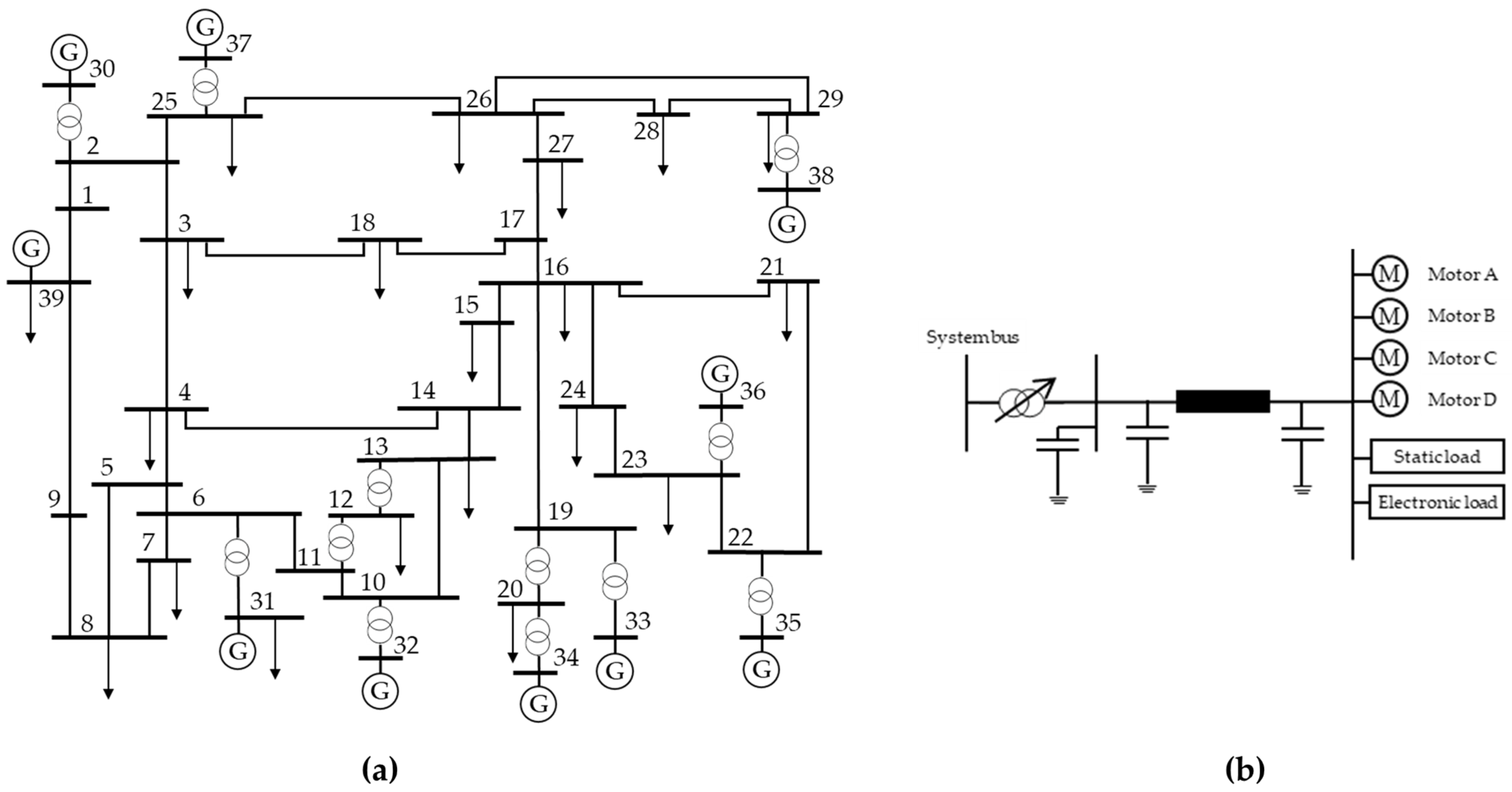
The RMS simulations were conducted in DIgSILENT PowerFactory within the IEEE 39-bus New England system, as illustrated in Figure 3 on the left. All loads were substituted with the WECC composite load model, as depicted in Figure 3 on the right. This was conducted in accordance with the prescribed active power and cos φ values, with the standard parameterization (proportion of motors A–D, in addition to electronic loads and ZIP loads, each accounting for 16.7% of the total load). A comprehensive account of the WECC load model can be found in [11]. Given the considerable proportion of dynamic load shares, the original grid loading (hereafter referred to as 100%) no longer results in the stable recovery of the voltage in any fault scenario. Consequently, the grid loading was reduced for these investigations. The simulated events involved three-phase short circuits in the middle of the lines under consideration, with a fault clearing time of 125 ms and without contingency propagations.

4.1. Grid Loading

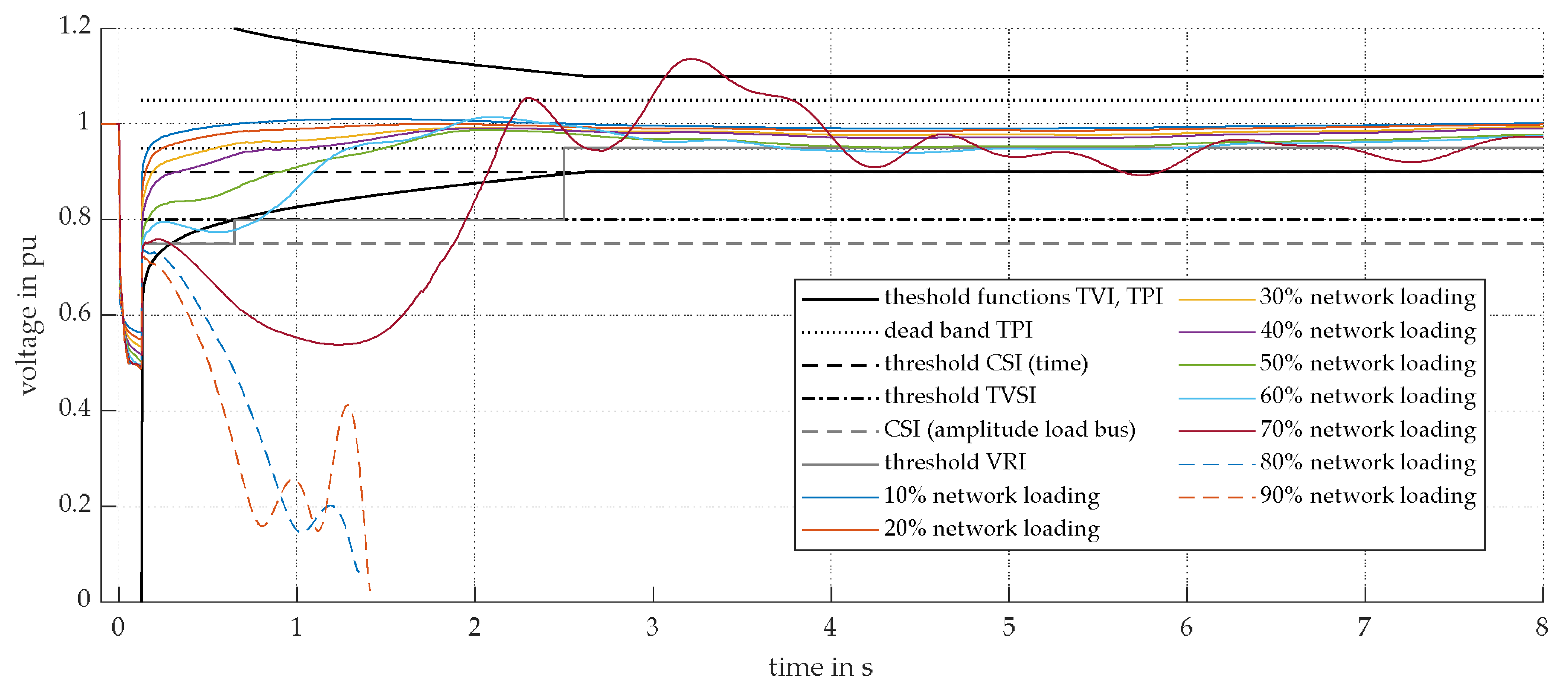
In the following, an increase in grid loading is examined. To do this, the power of the loads at a constant cos φ was increased in 10% steps, as was the active power fed in by the generators at the same voltage setting. The fault under investigation was located in the middle of line 03–04. Figure 4 shows the voltage curve for the different grid loadings at bus 6. As expected, the degree of criticality of short-term voltage stability increased with increasing grid loading. Up to 20% grid loading, the voltage curve still approximately showed the ideal form of a reciprocal exponential function and stabilized very quickly in the nominal voltage band range. At higher loadings, the FIDVR effect became more and more pronounced, which is favored by the high proportion of motor loads in the grid. At 70% loading, the voltage just managed to stabilize but oscillated to a large extent. Beyond that point, it was no longer possible to stabilize the voltages. In this case, the low oscillating voltages were caused by rotor instability. It is clear that the maximum voltage deviations after the fault clearance increased exponentially with increasing load on the grid and not linearly. This shows clearly that the closer the network load is to the critical level, the more strongly the voltage curves react to a disturbance.

To compare the different indices, the threshold values used must first be defined in a comparable way (see also Figure 4):

• For the TPI, set ${\mathrm{v}}_{\mathrm{l}\mathrm{t},\mathrm{s}\mathrm{t}\mathrm{a}\mathrm{t}}=0.95 \mathrm{pu}$ and ${\mathrm{v}}_{\mathrm{u}\mathrm{t},\mathrm{s}\mathrm{t}\mathrm{a}\mathrm{t}}=1.05 \mathrm{pu}$;
• For the TPI and the TVI, set ${∆\mathrm{v}}_{\mathrm{l}\mathrm{o}\mathrm{n}\mathrm{g}}=0.05 \mathrm{p}\mathrm{u}$; $\mathsf{\beta }=0.05$ and ${∆\mathrm{t}}_{\mathrm{e}\mathrm{n}\mathrm{d}}=2.5 \mathrm{s}$;
  For the TVSI, the threshold value is set to $0.8 \mathrm{p}\mathrm{u}$;
• For the CSI, the threshold value (in contrast to [4]) for the voltage sag duration was $0.9 \mathrm{p}\mathrm{u}$, the weighting factors were both 0.5, and the threshold value for the amplitude of the voltage sag was as in [4] at $0.75 \mathrm{p}\mathrm{u}$ for a load bus and $0.6 \mathrm{p}\mathrm{u}$ for all other nodes;
• For the VRI, the stepwise limit function was defined as follows: $0.75 \mathrm{p}\mathrm{u}$ until $0.65 \mathrm{s}$; $0.8 \mathrm{p}\mathrm{u}$ until $2.5 \mathrm{s};$ and $0.95 \mathrm{p}\mathrm{u}$ beyond. All other parameters were also selected according to [7].

The simulation results in the various indices calculated for bus 6 at different grid loadings is shown in

Table 2. Values for various indices at bus 6 for various grid loadings in the event of a fault on line 03–04.

Grid Loading	${\mathbf{C}\mathbf{S}\mathbf{I}}_{\mathbf{b}\mathbf{u}\mathbf{s}6}$	${\mathbf{T}\mathbf{V}\mathbf{S}\mathbf{I}}_{\mathbf{b}\mathbf{u}\mathbf{s}6}$	${\mathbf{T}\mathbf{V}\mathbf{I}}_{\mathbf{b}\mathbf{u}\mathbf{s}6}$	${\mathbf{V}\mathbf{R}\mathbf{I}}_{\mathbf{b}\mathbf{u}\mathbf{s}6}$	${\mathbf{T}\mathbf{P}\mathbf{I}}_{\mathbf{b}\mathbf{u}\mathbf{s}6}^{+}$	${\mathbf{T}\mathbf{P}\mathbf{I}}_{\mathbf{b}\mathbf{u}\mathbf{s}6}^{-}$
10%	0	0	0	0.3295	0.1530	0
20%	0	0	0	0.3441	0.2575	0
30%	0	0	0	0.3270	0.3380	0
40%	0	0	0	0.3049	0.4134	0
50%	0.0441	0.0266	0	0.2518	0.5216	0
60%	0.0606	1.1325	0.0016	0.2232	1.0644	0
70%	0.4421	11.5995	0.4974	0.0055	5.2989	−0.7007
80%	0.9898	79.9186	3.8922	−0.1297	18.5312	0
90%	0.9941	86.0381	4.1078	−0.1580	18.7733	0

, and for the entire grid in

Table 3. Maximum indices occurring in the network (minimum for VRI) in the event of a fault on line 03–04 for different grid loadings; the value in brackets indicates the most critical bus in each case.

Grid Loading	${\mathbf{C}\mathbf{S}\mathbf{I}}_{\mathbf{b}\mathbf{u}\mathbf{s}6}$	${\mathbf{T}\mathbf{V}\mathbf{S}\mathbf{I}}_{\mathbf{b}\mathbf{u}\mathbf{s}6}$	${\mathbf{T}\mathbf{V}\mathbf{I}}_{\mathbf{b}\mathbf{u}\mathbf{s}6}$	${\mathbf{V}\mathbf{R}\mathbf{I}}_{\mathbf{b}\mathbf{u}\mathbf{s}6}$	${\mathbf{T}\mathbf{P}\mathbf{I}}_{\mathbf{b}\mathbf{u}\mathbf{s}6}^{+}$	${\mathbf{T}\mathbf{P}\mathbf{I}}_{\mathbf{b}\mathbf{u}\mathbf{s}6}^{-}$
10%	0	0	0	0.276 (32)	0.181 (32)	0
20%	0	0	0	0.279 (32)	0.287 (16)	0
30%	0	0	0	0.267 (31)	0.406 (16)	0
40%	0	0.027 (16)	0	0.250 (31)	0.502 (16)	0
50%	0.036 (16)	1.139 (25)	0	0.197 (28)	0.693 (21)	−0.226 (31)
60%	0.075 (16)	2.166 (16)	0.102 (16)	0.111(35)	1.300 (16)	−0.804 (31)
70%	0.339 (10)	12.867(9)	13.346 (9)	−0.012 (9)	6.122 (10)	−4.446 (31)
80%	0.793 (12)	80.525 (9)	87.393 (8)	−0.141 (5)	18.862 (12)	−3.444 (39)
90%	0.787 (14)	86.328 (12)	88.972 (12)	−0.177 (11)	19.897 (7)	−4.155 (39)

(value of the bus identified as most critical by the respective index).

As illustrated in Figure 4, the time-based representation of the voltages revealed that the threshold values of all indices were transiently exceeded at the latest at a grid loading of 60%. At grid loading levels of 80% and 90%, the grid was demonstrably unstable. The grey values in Table 2 indicate the loading at which the respective index’s threshold values were exceeded for the first time. The CSI, TVSI, TVI and TPI provided reliable indications of this violation, whereas the VRI continued to display a positive value at 60% grid loading. Consequently, a definitive statement regarding the exceedance of the limit was not possible within the threshold area. The issue of insufficient gradation within the permissible voltage range was evident in the case of CSI, TVSI, and TVI, where zero values were observed in the range preceding the threshold value. Consequently, it was not possible to ascertain the proximity of the value to the threshold value. In contrast, the grading of the VRI and TPI indices, even within the permissible voltage range, clearly demonstrated their advantage. In the context of this study, TPI⁻ can be considered as a supplement to TPI⁺ and may be particularly useful in situations where overvoltage problems in the grid are anticipated.

4.2. Most Critical Fault Locations in the Grid

In the context of a comprehensive analysis of the stability of a network, it can be a useful strategy to identify critical fault locations or regions in order to analyze their stability in more detail. In order to assess the efficacy of the indices in identifying the most critical fault location, simulations were extended to encompass other fault locations (comprising all existing lines and faults situated in the middle of the line) across a range of grid loading scenarios in five steps. 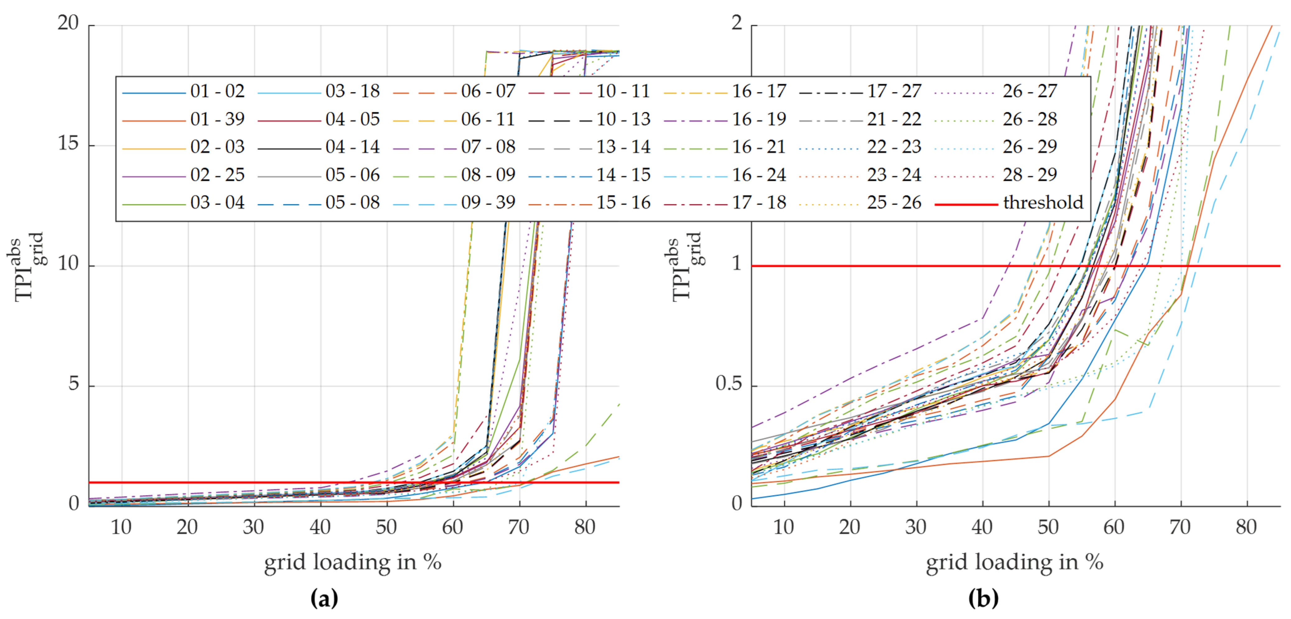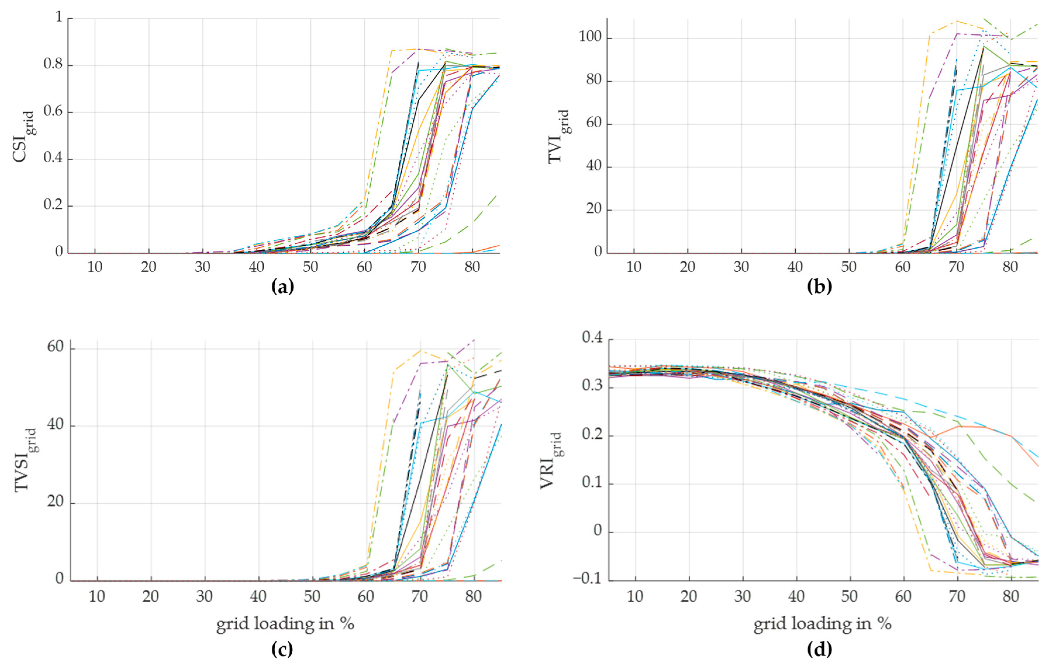Figure 5 illustrates the calculated TPI, while Figure 6 depicts the determined values for the CSI, TVI, TVSI, and VRI across the various scenarios, each based on the complete grid. As some fault locations were so problematic for the network that they no longer led to convergence in the simulation, even at loads below 80%, these values are missing in the evaluation.

The results demonstrate that the most critical fault locations identified for all indices exhibited a high degree of similarity.

Table 4. The most and least critical fault locations determined at a grid loading of 55%.

	TPIabs	CSI	TVI	TVSI	VRI
Most critical fault locations	Line 16–19, Line 16–24, Line 16–17	Line 16–19, Line 16–24, Line 16–17	Line 16–17, Line 16–24, Line 16–19	Line 16–24, Line 16–17, Line 16–19	Line 16–19, Line 16–24, Line 16–17
Least critical fault locations	Line 01–39, Line 09–39, Line 08–09	Line 01–02, Line 01–39, Line 08–09, Line 09–39	26 fault locations	Line 01–02, Line 01–39, Line 08–09, Line 09–39	Line 09–39, Line 08–09, Line 28–29

illustrates the three most and least critical fault locations identified by the various indices for a grid loading of 55%, which, in the simulation, represented the highest grid loading without convergence issues for specific fault scenarios. The issue with the CSI, TVI, and TVSI was evident from the outset: they continued to display values of 0 for specific fault locations, indicating that the threshold value had not been exceeded and that the indices were not triggered (highlighted in grey in Table 4). Consequently, it was not possible to rank the fault locations according to their criticality for these locations without conducting further simulations at higher grid loadings. The TPI and VRI offer a distinct advantage in this regard, as they facilitate the ranking of the most critical failure locations, even at lower grid loadings. This simplifies the selection of an appropriate grid loading for determining the criticality of individual failure locations and reduces the number of simulations required in individual cases.

All indices yielded the same three most critical failure locations (with minor deviations in the order) when determining the most critical failure locations.

5. Handling Uncertainties in Load Parameterization

In order to make a well-founded statement about the stability of a power system, it is essential that a grid operator is able to estimate the uncertainties associated with the grid’s input data. The input data can initially be classified into two categories:

• Operating equipment data;
• Grid usage case data.

The first category encompasses lines, transformers, reactive power sources, and generation systems, along with their dynamic models and parameters. It may be reasonably assumed that these parameters are known to the grid operators, as the operating resources fall within their area of responsibility and the operators of generation systems are obliged to provide the grid operators with the relevant data in accordance with the grid connection rules. It should be noted, however, that the data and models in question may be subject to uncertainty due to several factors. These include potential measurement inaccuracies, for instance, in the case of zero impedance measurements of transformers, the use of default values for missing data, such as in the case of overhead lines, and parameter fluctuations caused by external influences, such as weather effects on overhead lines.

The data pertaining to grid usage encompass all time-varying information necessary for the simulation of diverse scenarios within the power system. Grid usage case studies are typically conducted by network operators using forecasts and market simulations to assess the stability of the system in a future period and to identify potential grid reinforcements. In the context of transmission grids, loads represent the aggregated lower-voltage-level grid components, including lines, consumers, and decentralized generator systems, the majority of which are converter-based. As part of the energy transition, the latter have become so widespread, especially in Germany, that power is fed from the distribution grids into the transmission grids during many hours of the year. In the case of stationary grid calculations, the forecast of the active and reactive power exchange at the transmission bus between the transmission grid and the aggregated load is typically sufficient. However, their prognosis is also subject to the inherent uncertainties associated with such predictions. In particular, the determination of reactive power data is frequently facilitated by the utilization of AI programs, which are based on historically measured values. However, this presents a significant challenge, particularly in light of the rapid expansion of photovoltaic and wind power plants, which are highly susceptible to weather fluctuations.

In dynamic simulations, the number of parameters required for an adequate representation of the voltage- and frequency-dependence as well as the dynamic behavior of the loads increases significantly. Given the disparate reactions of individual devices and systems in the grid to changes in voltage and frequency, it is imperative that they be modeled in a manner that reflects their respective shares of the load composition with the greatest possible realism. In the existing literature, there are several load models that have been developed for use in dynamic short-term simulations. These include the exponential model, ZIP model, models for motor loads, and composite models. Of these, the WECC composite load model is undoubtedly the most complex that is currently documented in the literature, and correspondingly has a high number of parameters [18]. These classic load models are regarded as pure consumer models. In order to account for the feed-in from converter-based micro-plants in distribution networks, these models are being augmented with corresponding generator models. The present paper will, however, limit its scope to consumer models.

The adequate parameterization of these consumer models can prove to be an extremely complex and uncertain process when considered in the context of the following factors:

• It should be noted that sectors such as residential, industrial, and commercial areas can exhibit significant heterogeneity with regard to the device classes present. In the USA, conversely, the high penetration of air conditioning systems in the private sector has resulted in an increase in FIDVR events [19].
• The period of time during which certain device groups are utilized can vary considerably depending on the time of day, the day of the week, and the season. In the latter case, meteorological conditions are a particularly significant factor. For example, heating appliances are primarily used during the winter months and are increasingly being designed as heat pumps or electric heaters.
• Consumer devices, which range from the smallest devices in the private sector to large industrial motors, exhibit structural differences. The parameterization of consumer models for individual device types must reflect both the composition of the devices at an electronic level and the range of devices themselves as well as their technological development and corresponding penetration in the grid. Furthermore, cultural and geographical differences also influence the penetration of specific device types within the grid.

These considerations raise questions about the applicability of parameterization suggestions from the literature, particularly in light of their potential cultural and geographical limitations and the need to account for technological developments and the penetration of device types in the grid. An individual assessment of the parameterization for the grid operator can either be measurement-based (e.g., [12]) or component-based (e.g., [20]), with both methods having their respective advantages and disadvantages. An alternative would be to resort to standard parameterizations. Nevertheless, certain uncertainties remain in the parameterization, which need to be estimated.

In order to demonstrate the impact of parameterization uncertainties on the evaluation of grid criticality using indices, we present below a series of Monte Carlo simulations in which specific load parameters were varied according to a standard Gaussian distribution.

5.1. Uncertainties in Determining the Active Power of Loads

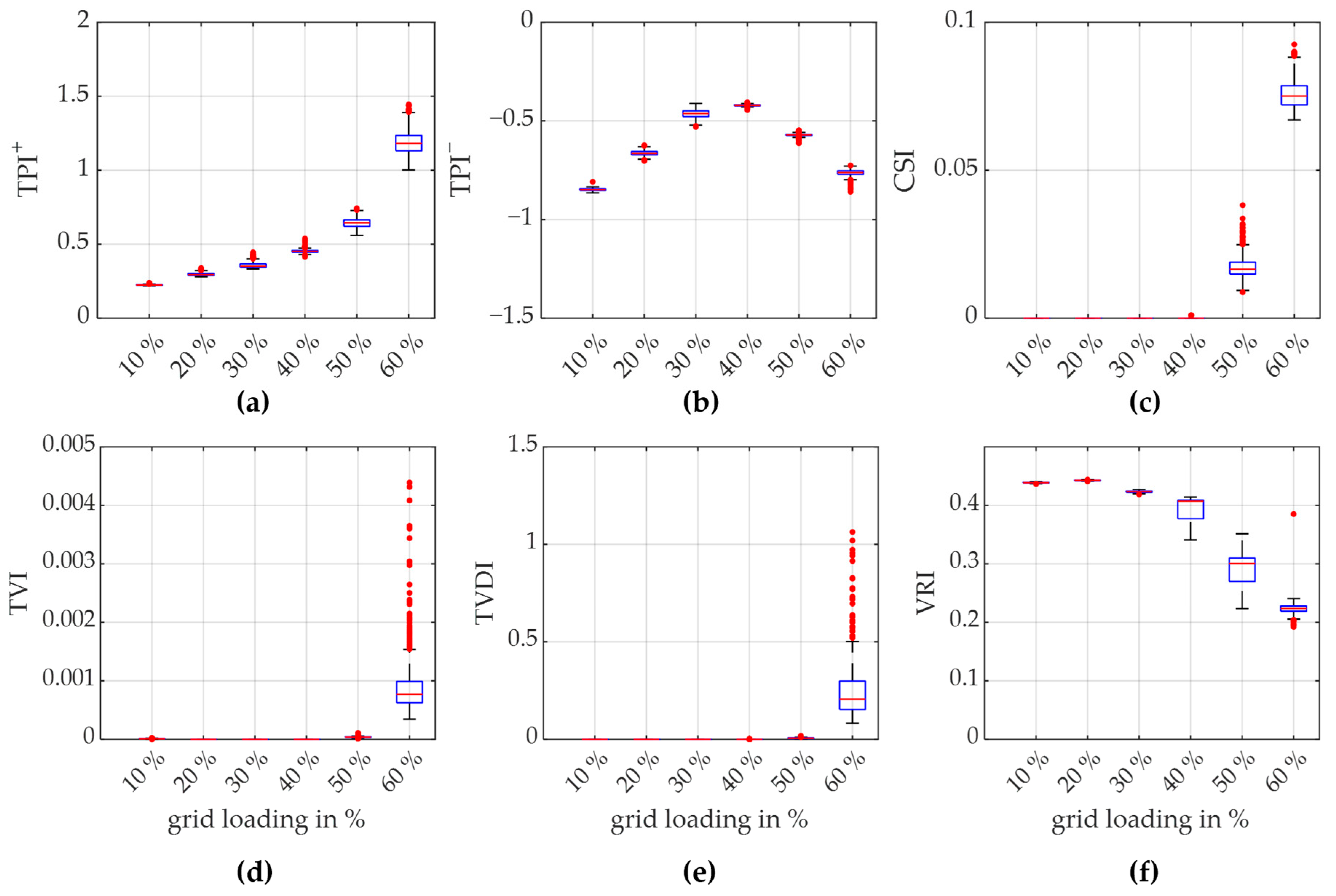
In the Monte Carlo simulations, the total active power of the individual loads was randomly varied according to a Gaussian distribution with a standard deviation of 10%. The value of the cos φ was retained, as was the parameterization of the WECC composite load model. For each grid loading scenario, approximately 500 simulation runs were calculated.

As illustrated in Figure 7, the outcome of the Monte Carlo simulation reiterated the shortcomings of CSI, TVI, and TVSI, which failed to activate at low grid loadings. In contrast to TPI and VRI, these indices failed to provide any indication of the proximity of the network to the specified voltage limit in these cases. Nevertheless, the Monte Carlo simulation can be employed to corroborate that the grid can be deemed sufficiently stable, even when the uncertainties are taken into account. Nevertheless, given the considerable computational and time demands of Monte Carlo simulations, they are not well-suited for the comprehensive and systematic analyses of real-world networks. In this context, the advantages of TPI and VRI were demonstrated by the fact that a simple simulation already provides information about the distance to the voltage threshold, and thus the criticality of the grid.

As the impact of uncertainties on stability increased with proximity to instability, the bandwidths of the respective indices determined in the Monte Carlo simulations became increasingly wide. In the context of the systematic and complete analyses of real networks, this indicates that grid usage cases with small TPI⁺ values (or large VRI values) can be assumed to be stably secured by a single simulation with a standard parameterization of the loads. For higher TPI⁺ values (or smaller VRI values), the wide range of indices to be considered, when taking into account the uncertainties, indicates the need for more detailed simulations or the utilization of a safety margin relative to the threshold value (TPI⁺ = 1 or VRI = 0).

5.2. Uncertainties in Determining the Parameters of Loads

The WECC composite load model has 131 parameters and is therefore significantly more complex than other load models [15]. The parameters can be divided into three categories:

• Substation and feeder parameters (relating to transformers, lines and compensation units);
• Shares of the individual load classes, to which the specified active power of the load is distributed;
• Sub-parameters of the individual load classes.

It has been shown that the parameters of the second category, in particular, exhibited high sensitivities in simulations with voltage dips [21,22]. Therefore, these should be varied in further Monte Carlo simulations as well as with a standard Gaussian distribution with a standard deviation of 10%. However, it must be taken into account that the sum of all load shares must equal one. In order to achieve this, the shares for motors A to D, the electronic loads, and ZIP loads were randomly selected and standardized to a sum of one.

Since the ZIP load combines loads with constant impedance (Z), constant current (I), and constant power (P), whose proportions are in turn controlled by parameters, these were varied according to the same principle. The variations of the parameters were carried out separately for each load bus. All other parameters were retained in accordance with the standard parameterization.

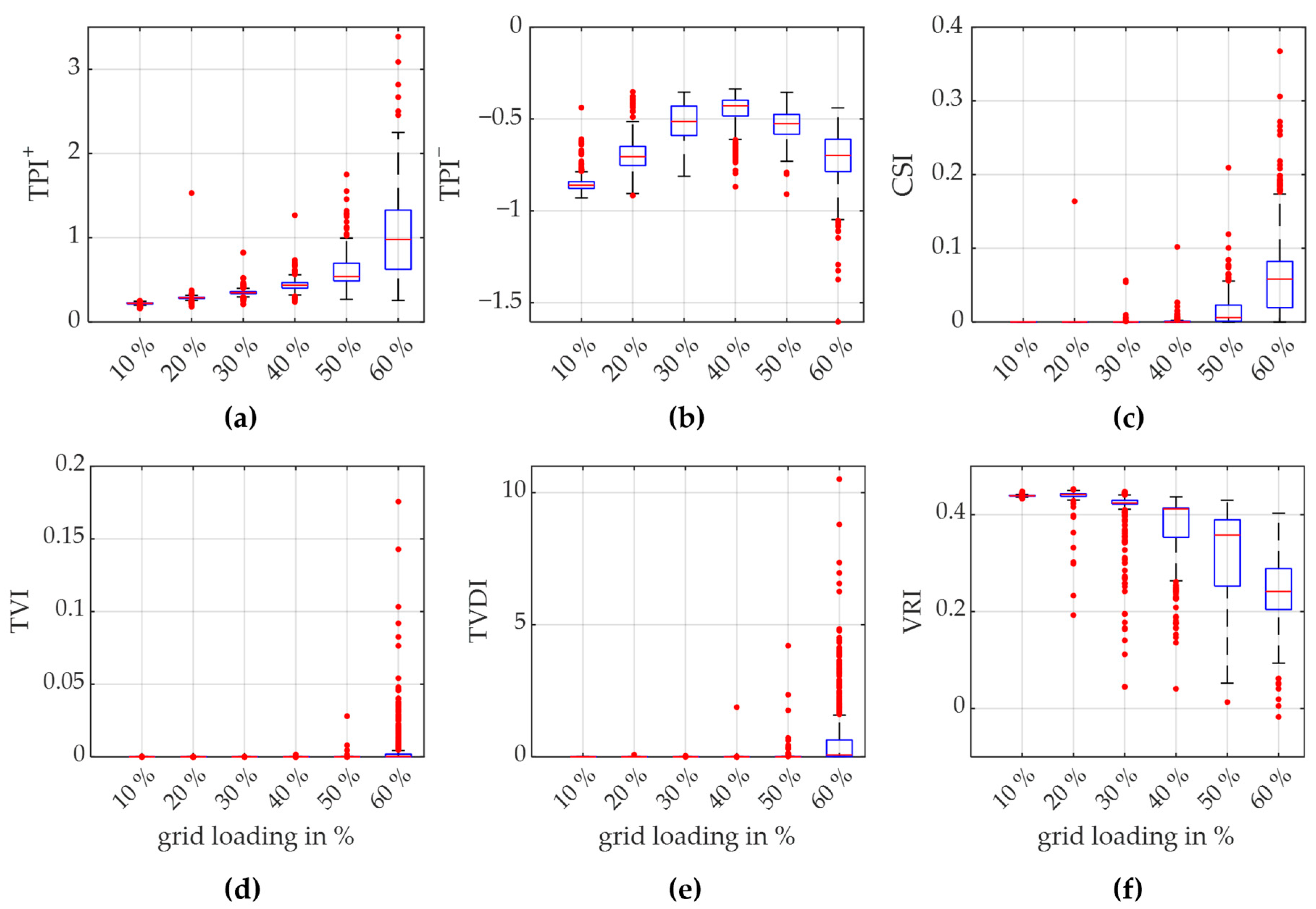
The resultant data from the Monte Carlo simulation are visualized in Figure 8. The results showed that the variation in the parameters exerted a markedly greater influence on grid stability than the variation in the active power of the loads. This demonstrates the importance of accurate load parameterization and the incorporation of load uncertainties in stability analyses for short-term voltage stability in real grids. This was particularly evident in the case of a grid loading of 60%, where the TPI⁺ in the Monte Carlo simulations had a mean value of approximately 1 but also a wide range in both directions. It is therefore evident that a single simulation with an arbitrary parameterization could rapidly result in misinterpretation in the context of real networks. Moreover, it highlights the challenging task of further work to define suitable security margins depending on assumed model accuracy.

It is recommended that network operators employ case-specific parameterizations in their simulations in order to reduce uncertainties. The standard deviation of 10% employed in this simulation is a relatively large value and was used for illustrative purposes only. The standard parameterization of the WECC composite load model, as employed in these simulations, exhibited a considerable proportion of motor loads that may not be present in real networks, thereby amplifying the results.

The differentiation between TPI⁺ and TPI⁻ is advantageous in this context, as it enabled the detection of even excessive voltages. For grid loadings up to 50%, no violations of the upper voltage limit values were observed. Nevertheless, the minimum values of the TPI⁻ indices in the Monte Carlo simulations, which approached −1, suggest that the stability of the grid may already be approaching the critical range, as was the case for individual parameterizations at 60% grid loading. Indeed, the overvoltage issues were considerably more pronounced than the undervoltage problems at grid loadings of up to 40%. This was evident from the separate display of the TPI⁺ and TPI⁻ indices. Furthermore, an evaluation of the TPI^abs would directly indicate the criticality of these grid loadings. The remaining indices incorporating upper voltage limit values, namely TVI and TVSI, were not activated in these instances, as anticipated. The CSI and the VRI lacked the capability to illustrate these surges.

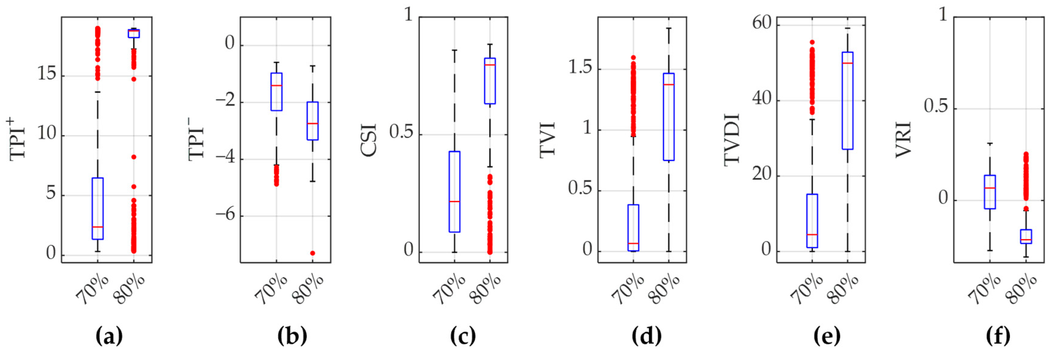
For a more comprehensive illustration, the simulation results for grid loadings of 70% and 80% are shown in a separate graphic in Figure 9. Given the prevalence of instabilities in these scenarios, notable values were particularly observed for the TPI, TVI, and TVSI. The maximum possible values for TVI and TVSI depend upon the selected time period utilized in the calculation of the indices, whereas the choice of voltage threshold and dead band is the determining factor for the maximum possible values of the TPI. Nevertheless, the results indicate that permissible voltage recoveries can still be achieved in a few parameter constellations with these grid loadings, which ultimately underscores the necessity for the precise parameterization of loads.

6. Conclusions and Outline

The objective of the analyses presented here was to identify an appropriate evaluation index for assessing the short-term voltage stability of an electrical power system in dynamic simulations for grid planning purposes. The stability of a grid is considered to be the ability to maintain voltage over a defined threshold after faults. In real grids, the high number of network use cases and possible fault locations leads to a high number of necessary simulations. When considering uncertainties in parametrization, this number increases further. In order to reduce the number of necessary simulations and facilitate the evaluation of stability, a metric was sought that provides an indication of the proximity of the voltage curve to the threshold curve. This and other requirements were listed and compared with indices from the literature.

This was demonstrated by means of theoretically deduction as well as a practical observation that none of the existing indices satisfied all of the necessary criteria, thus necessitating the development of a novel index, the threshold proximity index (TPI), which was found to meet all of the specified requirements. The TPI was tested using exemplary simulations and compared with other indices to demonstrate that the presented requirements and their implementation in the TPI are advantageous in the context under discussion.

The indices employed for comparison were the CSI, TVI, TVSI, and VRI, since they are all also based on threshold values and thus allow for a meaningful comparison. The CSI, TVI, and TVSI were designed to evaluate the severity of exceeding a threshold value; if no threshold value is exceeded, they always return with a value of zero. Consequently, in stable situations, they do not provide any information about the proximity of the threshold value. Conversely, the VRI, akin to the TPI, evaluates the distance of the voltage from the limit value curve. While the TPI solely appraises the maximum proximity or exceedance of the threshold curve, the VRI quantifies this with the aid of various weightings over the entire period under consideration. In scenarios where critical fault locations are sought or where evaluating the stability is coupled with uncertainties, the early triggering of an index in non-critical situations is of significant benefit. The capability to evaluate voltage recovery, even in stable scenarios, facilitates the comparison of diverse grid scenarios. It enables the identification of stable yet critical situations (i.e., scenarios where the voltage approaches the threshold value). Conversely, it can also discern situations that are entirely non-critical, thereby circumventing superfluous simulations aimed at assessing uncertainties. As demonstrated in the simulations presented, both the TPI and the VRI were able to show the advantage of evaluating the distance from a threshold value in stable situations in comparison with the CSI, TVI, and TVSI.

Even though the VRI was proven to be quite advantageous in the simulations, this index is not without certain disadvantages. The threshold value function is designed in stages, which does not align with the natural continuum of voltage recovery and does not incorporate upper voltage limits. Furthermore, it should be noted that the index does not offer an unequivocal assurance that the voltage is or is not in excess of the threshold in borderline scenarios. Moreover, it is encumbered by the challenging parameterization of the index itself.

The TPI is supposed to form the basis for a systematic investigation of the short-term voltage stability of electrical networks, with due consideration of the uncertainties. These investigations could be made up of individual steps to identify important network regions and situations and to find critical combinations. To do this, we need to define what ’critical’ means in the context of the grid. Using the TPI, this must then be transferred into the formulation of the threshold functions. Finally, the critical combinations should also be checked for uncertainties in the parameterization, especially the dynamic load models. In the end, a decision needs to be made about whether the network is stable enough, or if it needs to be reinforced. Given the considerable computational demands of dynamic simulations, it is prudent to limit the number of simulations to a minimum while ensuring that critical system states are not overlooked. The analyses carried out here show that the use of the TPI is of decisive advantage. However, we believe that the TPI can also be applied to other analytical problems such as finding the best location for dynamic reactive power sources to support short-term voltage stability.

Further development and improvement of the TPI is a possibility, particularly with regard to increasing the penalty for voltage values approaching the threshold value function. This would better reflect the nonlinear relationship between criticality (in this case, grid loading) and voltage dips. In order to facilitate greater standardization, it would be advantageous to limit the output values of the TPI in the unstable range to a fixed value, for example, 2 or −2. Furthermore, by eschewing the joint assessment of upper and lower threshold values, it would be possible to shift the value range to the range from +1 to −1, in accordance with the VRI.

These improvements and the use of the TPI in the context of systematic network stability investigations as well as the definition of suitable reliability margins for TPI will be the subject of future publications.