Different modeling approaches were applied for each soil type: logarithmic functions, polynomial models of varying degrees, power law fitting, cubic spline interpolation, radial basis functions (RBF), penalized regressions (LASSO and RIDGE), segmented models (breakpoints), and nonparametric smoothing using LOESS. The selection of the optimal model was based on goodness-of-fit criteria (coefficient of determination ), minimization of the root mean square error (RMSE), and cross-validation to avoid overfitting.
Each section presents the analysis and fitted models for each soil type. Scatter plots, fitted curves, derived equations, and evaluation metrics are included.
3.3.1. Sandy Soil
The experimental values and fitted models for the sandy soil are presented in
Table 5. This table shows the measured electrical resistivity as a function of gravimetric moisture content, from 5% to 100% (excluding 0% due to its extreme value).
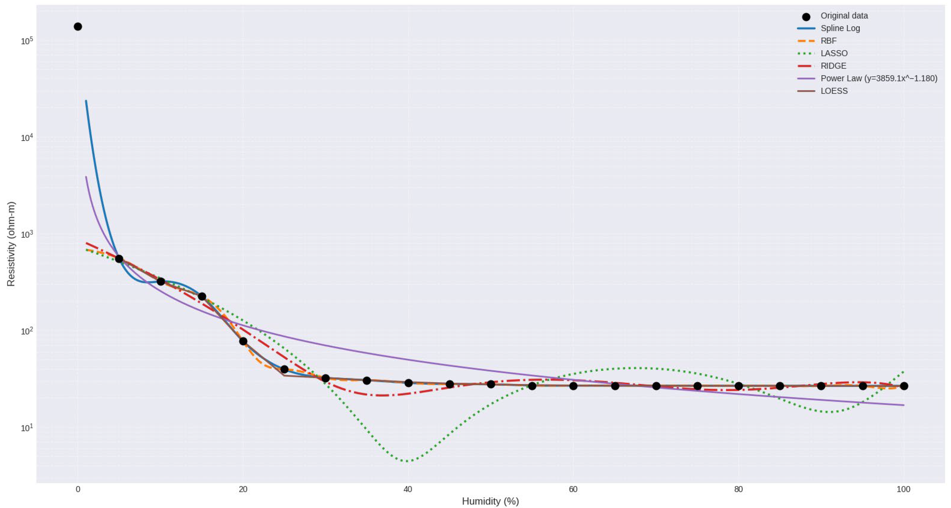
Overall, the Spline-Log and RBF models accurately reproduce the actual values, matching each point exactly, reflecting a near-perfect fit. These models are particularly effective at capturing nonlinear behavior and the abrupt resistivity transition between 5% and 25% humidity, a critical zone where there is a sharp drop in resistivity (from 555.04 to 39.52 ).
The LASSO model tends to slightly underestimate values between 5% and 20% moisture content and overfit in intermediate ranges (30% to 60%), showing fluctuations that do not correspond to the experimentally observed pattern. On the other hand, the RIDGE model presents a good overall fit; however, it shows some significant deviations, especially between 15% and 25%, where it deviates notably from the actual values, with deviations of up to 100 . This suggests a low capacity to capture the nonlinear behavior of sandy soil under these conditions.
The Power Law model shows a good fit in the intermediate humidity ranges (25–60%), but overestimates resistivity under dry conditions and underestimates it under saturated conditions, with a progressive bias. Finally, the segmented equation shows good overall performance with small deviations, particularly in the critical zone between 15% and 20%, where it most faithfully replicates the inflection points in the humidity–resistivity curve.
Overall, the Spline-Log and RBF models are the most accurate and stable across the entire humidity range, making them suitable for representing the behavior of sandy soil, which is characterized by an exponential decrease in resistivity with increasing humidity until stabilizing at values close to 26.6 under saturation conditions (≥65%). On the other hand, the RIDGE, potential, and segmented models provide values for basic approximation.
Figure 6 illustrates the relationship between electrical resistivity and gravimetric moisture content for sandy soils, along with the fitted mathematical models. The black dotted curve represents the experimental values obtained in the laboratory. The fitting curves correspond to the following models: Logarithmic Spline, RBF, LASSO, RIDGE, and Power Law.
Models that present explicit equations include the Power Law model and the segmented equation model. These formulations allow the description of soil electrical resistivity as a direct function of gravimetric moisture content. The corresponding expressions are as follows:
Segmented Equation:
where
and
are indicator functions that equal 1 if the condition is met and 0 otherwise.
Table 6 shows the comparison of the fit metrics for each model, revealing the significant differences in accuracy and predictive capacity.
In the case of sandy soils, the Spline-Log and RBF models proved to be the most accurate, achieving an = 1.00 and zero error (RMSE = 0.00, MAE = 0.00, MA-PE = 0.00%), indicating a perfect fit to the experimental data. However, it should be noted that these models involve a higher degree of computational complexity, which may limit their applicability in scenarios where rapid or manual estimation is required.
In contrast, models with explicit expressions, such as Power Law and Segmented Equation showed inferior fit performance, = 0.95 and 0.91, respectively, and MAPE of 39.60% and 6.14%, implying a larger margin of relative error particularly for the Power Law model. Nevertheless, these formulations are valuable for their ease of use in manual calculations or quick applications.
Figure 7 presents the absolute error behavior of each model at different levels of gravimetric moisture content allowing us to identify its local accuracy. As can be seen, the Spline-Log and RBF models perform perfectly with an absolute error of zero at all points evaluated, confirming their excellent fit as previously noted.
The LOESS model also maintains minimal absolute errors (<1 ) at almost all levels with slight deviations only between 25% and 60% humidity, demonstrating a very robust adjustment capacity, although slightly lower than the two previous models.
In contrast, the Power Law model exhibits high errors especially between 10% and 30% moisture content with a maximum of 67.0 at 15%, representing a significant overestimation in low-moisture soil conditions. These errors decrease as moisture content increases but remain considerable.
The LASSO model exhibits erratic behavior with high errors ranging from 5% to 25% peaking at 49.2 at 20% humidity. Above 35% humidity the error tends to stabilize below 15 , although certain fluctuations persist, reducing its reliability.
For its part, the RIDGE model exhibits an intermediate pattern: errors lower than those of LASSO and Power Law, but still higher than LOESS with a maximum value of 35.3 at 15% humidity.
It is important to note that the predictive model for sandy soil is strictly valid within the experimentally determined gravimetric moisture range (5–100%). Within this interval, the model accurately reproduces the resistivity–moisture relationship, while extrapolation beyond these limits (especially under conditions of extreme dryness or saturation) can introduce uncertainty due to the nonlinear behavior of the soil. Therefore, predictions near or outside these limits should be interpreted with caution.
3.3.2. Clay Soil
The numerical results obtained for the clayey soil in a moisture content range between 5% and 100% are shown in
Table 7. These results allow us to evaluate the predictive capacity of the different models used in the study. As can be seen in
Table 7, the Logarithmic Spline and RBF models accurately reproduce the actual values at all moisture content levels. However, this accuracy may suggest overfitting or excessive dependence on the training set and should therefore be interpreted with caution when extrapolating results.
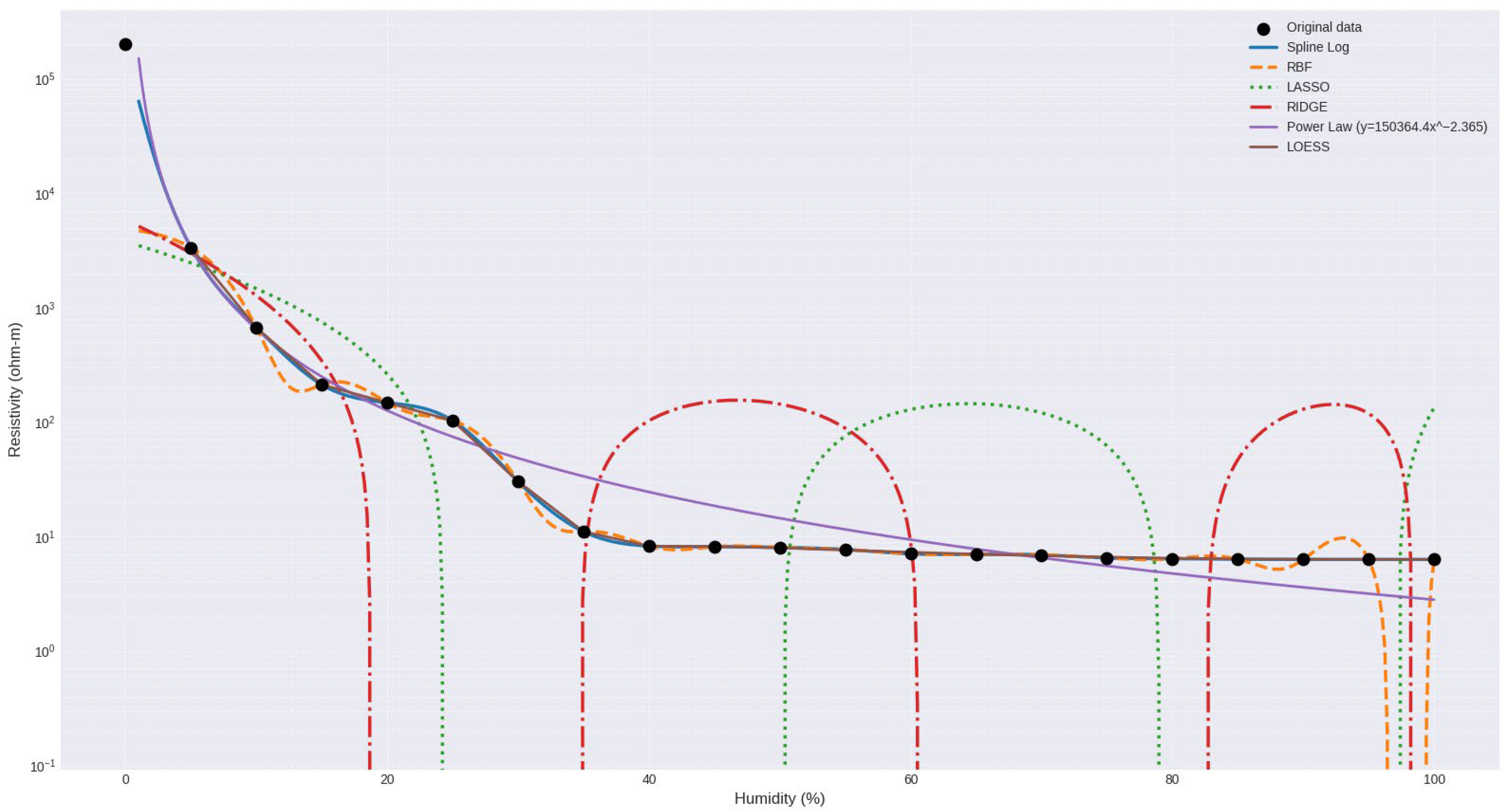
In contrast, the LASSO model shows significant deviation from actual values, especially at low and medium humidity levels, where even negative values are generated, which is physically meaningless in this context. This behavior indicates that the LASSO model has significant limitations in capturing the nonlinear behavior of resistivity with humidity, particularly in its critical transition zone.
The RIDGE model performs better than LASSO, although it also presents significant errors. While it more closely follows the decreasing trend in resistivity with increasing humidity, it experiences abrupt fluctuations with negative values starting at 20% humidity (e.g., −168.34 at 25%) and unexpectedly high values in the saturation zone (e.g., 151.77 at 45%).
The Power Law model offers predictions reasonably close to actual values in the initial humidity ranges (5–30%), but its accuracy decreases as the saturation zone increases. Above 30% humidity, the model tends to slightly overestimate values, although it always maintains physically valid results. This reinforces its usefulness as a generalizable explicit model, although it is not as accurate as other nonparametric approaches.
Finally, the segmented equation model exhibits adequate performance in both moisture content zones (hydration zone and saturation zone). Although it does not match the accuracy of Spline or RBF, it maintains contained errors and avoids extreme or inconsistent values. For example, it predicts 243.60 at 15% humidity (compared to a real 211.83 ) and 5.24 at 100% humidity (compared to a real 6.29 ), indicating a satisfactory fit within an explicit functional framework.
Taken together, these results reinforce that while nonparametric models offer superior accuracy for comprehensive datasets, explicit models, such as the Segmented Equation or Power Law, are valuable for their interpretability and general applicability.
Figure 8 shows the curve relating electrical resistivity and gravimetric moisture content for the clayey soil, along with the fitted mathematical models. The curve with black dots represents the experimental values obtained in the laboratory. The fitted curves correspond to the following models: Logarithmic Spline, RBF, LASSO, RIDGE, and Power Law.
The models that present explicit equations are the power-law model and the segmented equation model. These formulations allow the electrical resistivity of the soil to be described as a direct function of gravimetric moisture content. The corresponding expressions are as follows:
According to the expression defined in Equation (3), the segmented equation is:
where
and
are indicator functions that equal 1 if the condition is met and 0 otherwise.
Table 8 shows the comparison of the fit metrics for each model, highlighting the significant differences in accuracy and predictive capacity.
In the case of clayey soil, the fitting models show considerable variability in their ability to reproduce the actual electrical resistivity values as a function of gravimetric moisture content. The Spline-Log, RBF, and LOESS models show a perfect fit with a coefficient of determination () of 1.00 and practically zero errors (RMSE = 0.00 and MAE ≈ 0.00 for Spline-Log and RBF; RMSE = 0.07 and MAE = 0.04 for LOESS), demonstrating high fidelity to the experimental data. However, their use is limited to computational contexts due to the lack of explicit equations.
In contrast, models with explicit formulations, such as the Power Law model and the segmented equation model, show remarkably acceptable performance. The Power Law model stands out with an of 0.99, an RMSE of 14.49, and a MAPE of 52.7%, positioning it as a valuable tool for analytical calculations with low computational dependency. The segmented equation model, meanwhile, achieves an of 0.93 with a MAPE of 15.1%, improving in accuracy relative to the Power Law model, albeit with a slightly higher RMSE.
The LASSO and RIDGE models exhibit poorer fit, especially LASSO, with a MAPE of over 1000%, which limits their practical usefulness in this type of soil. This behavior is also reflected in their predictions, where at several points they present negative values or values far from the expected magnitude.
In summary, for clayey soils, models based on smoothing techniques such as Spline-Log, RBF, and LOESS offer the best predictive capacity, while the Power Law model and the segmented equation remain useful alternatives in contexts where an explicit mathematical expression is required.
Figure 9 presents a heat map depicting the absolute error as a function of moisture level for each of the models evaluated in the clayey soil. The Log-Spline and RBF models show zero absolute error at all moisture levels, reflecting an adequate fit. The LOESS model also exhibits negligible errors (≤0.2
) across the entire moisture range, reinforcing its high accuracy, as reported in the global metrics.
In contrast, the LASSO and RIDGE models exhibit substantially higher errors across the entire humidity range, with maximum values of 882.1 and 604.5 , respectively, suggesting heightened sensitivity to low humidity conditions. As moisture content increases, the error decreases markedly in both models, although significant variability remains.
The Power Law model, while exhibiting larger errors than pure nonlinear models, offers acceptable performance, with errors below 40 at all humidity levels. The LOESS, Spline-Log, and RBF models offer superior and stable performance, while LASSO and RIDGE are less reliable.
It is important to note that the predictive model for clay soils is strictly valid within the experimentally determined gravimetric moisture range (5–100%). Within this interval, the model accurately reproduces the resistivity–moisture relationship, while extrapolation beyond these limits (especially under extremely dry or saturated conditions) can introduce uncertainty due to the nonlinear behavior of the soil. Therefore, predictions near or outside these limits should be interpreted with caution.
3.3.3. Silty Soil
The results for silty soils shown in
Table 9 indicate that most of the analyzed models exhibit good predictive performance in the hydration zone (5
20
) and in the saturation zone (moisture above 25
). However, some models show considerable deviations from the actual values.
The Spline-Log and RBF models again stand out for their accuracy, faithfully replicating actual values across the entire humidity range evaluated. This perfect match is due to the fact that both models directly interpolate the data and do not rely on an explicit equation, making them ideal benchmarks for comparison, although their applicability is limited in the absence of computational tools.
The RIDGE model maintains a good general approximation, with values close to the real ones, especially at humidity levels below 20%. However, it tends to overestimate resistivity at humidity levels above 30%, which is reflected in increasingly divergent predictions towards 100% humidity.
The Power Law model, while offering an explicit and easy-to-apply structure, exhibits significant overestimation at all humidity levels. Despite this deviation, its behavior is continuous and decreasing, maintaining its relative usefulness calculations with wide safety margins.
In contrast, the LASSO model presents inconsistent predictions with negative values in the range between 35% and 95% humidity, which shows a loss of predictive capacity and disqualifies it for application in this type of soil without reformulation.
For its part, the segmented equation maintains a more balanced performance, with low errors in the hydration zone and an acceptable fit in the saturation zone. Although it does not perfectly replicate real values, its predictions remain within physically reasonable ranges, and its explicit structure allows its use as an estimation tool.
Overall, the Spline-Log and RBF models stand out for their accuracy, while among the explicit models, the segmented equation offers the best relationship between accuracy and operational applicability in silty soils, followed by the Power Law model.
Figure 10 shows the relationship between electrical resistivity and gravimetric moisture content for the silty soil, along with the fitted mathematical models. The curve with black dots represents the experimental values obtained in the laboratory. The fitting curves correspond to the following models: Logarithmic Spline, RBF, LASSO, RIDGE, and Power Law.
Models that present explicit equations include the power-law model and the segmented equation model. These formulations describe the electrical resistivity of the soil as a direct function of gravimetric moisture content. The corresponding expressions are as follows:
According to the expression defined in Equation (3), the segmented equation is:
where
and
are indicator functions that equal 1 if the condition is met and 0 otherwise.
Table 10 shows the comparison of the fit metrics for each model, highlighting the significant differences in accuracy and predictive capacity.
The analysis of the metrics for the models applied to the silty soil confirms the findings observed in the numerical results. The Spline-Log and RBF models again achieved the best metrics (RMSE, MAE, and MAPE of 0, and equal to 1), indicating an exact fit to the input data. However, as mentioned above, their use may be limited by the need for specialized software when applied outside the modeling environment.
The LOESS model is among the methods that do not present explicit equations, showing minimal errors (RMSE = 0.48, MAE = 0.26, and MAPE = 2.60%) and an adequate coefficient of determination.
On the other hand, among the models with explicit expressions, the segmented equation offers the most balanced performance, with an MAPE of 13.16% and an of 0.89. Although its errors are higher compared to LOESS, it maintains reasonable accuracy.
The RIDGE model, with a MAPE of 36.90%, also shows a good fit ( = 0.99), although its absolute errors (RMSE = 17.48, MAE = 9.86) are more pronounced than in clayey soils. Even so, it could be considered an alternative when a balance between accuracy and simplicity is required.
The LASSO model, despite having a high (0.97), records a very high MAPE (124.50%). This indicates that, although it generally follows the data trend, its individual predictions are highly dispersed and, in some cases, unreliable, making it the model with the poorest performance, as it even predicts negative values. The Power Law model, although it shows a good coefficient of determination (0.96), has a MAPE exceeding 187%, revealing a substantial overestimation relative to the actual values.
The segmented equation offers relatively acceptable performance given its explicit nature and its potential use in calculations without requiring advanced modeling tools. With an RMSE of 19.63, an MAE of 12.32, and an MAPE of 13.16%, this model demonstrates acceptable accuracy, particularly in the high-humidity range, where predictions are remarkably close to actual values. The coefficient of determination ( = 0.89), although lower than those obtained with more complex models, still indicates a strong correlation between the independent variable (gravimetric moisture) and the dependent variable (electrical resistivity).
Overall, for silty soils, the Spline-Log, RBF, and LOESS models offer high accuracy, while the segmented equation and RIDGE models stand out as the most viable options when seeking a balance between applicability and acceptable error margins. However, the LASSO and Power Law models have error percentages that are too high for calculations requiring high precision.
Figure 11 illustrates the absolute error behavior for each model as a function of moisture content in silty soil. As in the other cases, the Log-Spline and RBF models perform exceptionally well, suggesting a complete fit to the training data. The LOESS model exhibits minimal errors—less than 1.5
across the entire analyzed interval—consolidating its accuracy and stability.
On the other hand, the Power Law model shows the largest errors at low humidity levels (10% to 30%), with a progressive decrease as humidity increases, eventually reaching near stabilization. The LASSO model displays an erratic pattern, with high errors (up to 78.9 ) at low humidity levels and intermediate error peaks, reflecting its sensitivity to the nonlinearity of the humidity–resistivity relationship.
In contrast, the RIDGE model exhibits more consistent behavior, with errors progressively decreasing to values below 5 at higher moisture levels. This analysis further demonstrates that models based on nonparametric and flexible techniques, such as LOESS, RBF, and Log-Spline, provide greater reliability for predicting electrical resistivity in silty soils, particularly under variable moisture conditions.
It is important to note that the predictive model for silty soils is strictly valid within the experimentally determined gravimetric moisture range (5–100%). Within this interval, the model accurately reproduces the resistivity–moisture relationship, while extrapolation beyond these limits (especially under extremely dry or saturated conditions) can introduce uncertainty due to the nonlinear behavior of the soil. Therefore, predictions near or outside these limits should be interpreted with caution.
The segmented equations were designed to consider two distinct humidity regimes observed in the experimental data: the hydration zone (low humidity) and the saturation zone (higher humidity). In the hydration zone, resistivity decreases sharply as water progressively fills the pore spaces, enhancing ionic mobility and electrical conduction. In contrast, the saturation zone represents a condition in which most conductive pathways are already established, resulting in a slower resistivity decline [
13,
14,
15]. The transition point, identified at approximately 25% for sandy and silty soils and 30% for clayey soils, corresponds to the onset of continuous water films and percolation paths within the soil structure.
Logarithmic terms were applied in the hydration zone to capture the rapid decrease in resistivity with small increases in moisture, while power-law terms were employed in the saturation zone to represent the slower decrease. Breakpoints were determined from inflections in the measured resistivity curves, indicating transitions in the dominant driving mechanisms [
17,
28,
34]. A limitation of the segmented equations is that, while empirically fitted and physically based, the choice of functional forms and breakpoints is specific to the soils studied. Extrapolation to other soil types or conditions should be undertaken with caution, and further validation is recommended.
In the segmented equations, moisture content is expressed directly as percentage units in logarithmic and power-law terms for convenience. Users should note that the models are validated only within the 5–100% moisture range, and numerical instability may arise if values outside this range are applied. Future work could explore normalization or dimensionless scaling to enhance numerical robustness.
Although LASSO and RIDGE regression models provide stability against overfitting and multicollinearity, their underlying linear structure limits their ability to capture the strong nonlinear dependencies between resistivity and moisture content. In soils, particularly clayey and silty types, electrical conduction mechanisms change nonlinearly with pore water distribution, ion mobility, and degree of saturation. The regularization terms (L1 for LASSO and L2 for RIDGE) enforce smooth and monotonic trends, which restricts the models’ responsiveness to abrupt resistivity variations across moisture regimes. Consequently, these models tend to underfit at extreme moisture levels and may yield physically unrealistic predictions. These anomalies result from overfitting in these nonparametric statistical models [
47,
49]. Consequently, caution should be exercised when interpreting these predictions. Future work could include constraints or physics-informed modeling to prevent such artifacts.
While the empirical equations derived from the explicit models in this study are strictly valid for the specific soil samples analyzed (classified as SP, CL, and ML according to the U.S. Soil Classification System), these models offer a computationally simple method for situations where advanced software and extensive databases are unavailable. Although site-specific calibration is recommended, these models could be used as reference curves to guide initial design considerations once validated through field studies.
It is important to note that although the Spline and RBF models yielded near-zero errors within the experimental dataset, their accuracy is a direct result of their interpolative nature. Consequently, they lack predictive capacity outside the tested range and should not be extrapolated to different soil conditions or moisture regimes without external validation. These limitations highlight the importance of developing and testing explicit models that can retain predictive reliability under variable field conditions.
Another limitation of this study is that, due to the use of a single sample per soil type, it was not possible to separate the data into independent training and test sets. While cross-validation techniques were applied to mitigate overfitting, the reported performance metrics (, RMSE, MAE) may be slightly optimistic. Therefore, the predictive models should be interpreted primarily within the context of the experimental data.
Another limitation is that MAPE can generate exaggerated errors at high humidity levels due to resistivity values close to zero, which may distort the model’s accuracy in this range. Future studies should consider alternative or complementary error metrics to avoid bias in performance assessment.
Although the Power Law model showed a high coefficient of determination, its error metrics revealed strong deviations in certain soil types, particularly silty soils. This discrepancy underscores that a high R2 alone is insufficient to establish predictive reliability. The segmented equation was prioritized because it offered a more consistent balance between accuracy, error distribution, and physical plausibility across soil types.
Another limitation of this study is that only one resistivity measurement was performed for each increment in gravimetric moisture content. While this procedure allowed for the characterization of the general relationship between soil moisture and resistivity, it limited the assessment of measurement variability and reproducibility. Consequently, it was not possible to report error bars or variability metrics. Therefore, future studies should incorporate replicate measurements to assess repeatability and improve the robustness of the data.
One limitation is that, although repeated measurements were performed to confirm the extremely high resistivity values observed in the 0% moisture samples, these results have not been validated using an independent measurement method. Future work should employ alternative instruments or field verification to further ensure the physical accuracy of these measurements.
Another limitation of this study is that the 0% gravimetric moisture measurement was excluded from the dataset, as it represented an extreme outlier with excessively high resistivity values, which could disproportionately affect model fitting. While this removal was necessary for the robustness of model development, it may limit the evaluation of model performance under very low moisture conditions.
A possible limitation of this study is that the manual homogenization of soil moisture, without mechanical mixing or a rest period, may have introduced minor non-uniformities in water distribution, potentially affecting the accuracy of resistivity measurements.
A limitation of this study is that the ±2% accuracy of the moisture sensor introduces uncertainty that may affect the precision of the predictive models, particularly at low moisture contents.
