A Nonlinear Extended State Observer-Based Load Torque Estimation Method for Wind Turbine Generators

Abstract

As global demand for clean and renewable energy continues to rise, wind power has become a critical component of the sustainable energy transition. However, the increasingly complex operating conditions and structural configurations of modern wind turbines pose significant challenges for system reliability and control. Specifically, accurate load torque estimation is crucial for supporting the long-term stable operation of the wind power system. This paper presents a novel load torque estimation approach based on a nonlinear extended state observer (NLESO) for wind turbines with permanent magnet synchronous generators. In this method, the load torque is estimated using current measurements and observer-derived acceleration, thereby eliminating the need for torque sensors. This not only reduces hardware complexity but also improves system robustness, particularly in harsh or fault-prone environments. Furthermore, the stability of the observer is rigorously proven through Lyapunov theory using the variable gradient method. Finally, simulation results under different wind speed conditions validate the method’s accuracy, robustness, and adaptability.

1. Introduction

The development of human social production is inseparable from energy as a vital material foundation. With the growth of the world’s population and the improvement in human living standards, fossil fuels, which currently serve as the primary energy source, will be unable to meet future human demand due to their non-renewability [1,2,3]. Furthermore, the extraction of fossil fuels leads to ecological damage, which hinders the harmonious development of human society and the natural world. Against this background, wind energy, as an abundant, renewable, and clean energy source [4], plays a crucial role in the global transition of the energy structure, and installed wind power capacity has been continuously rising in recent years. Concurrently, with the continuous increase in individual wind turbine capacity and structural complexity, as well as their gradual deployment into harsh environments such as deep-sea locations, wind turbines are increasingly exposed to non-stationary loads arising from complex natural conditions [5]. Excessive loads can easily lead to generator failures, seriously compromising the safety and reliability of the turbine’s long-term operation [6,7,8]. Therefore, accurate load estimation is the key prerequisite for achieving wind turbine condition monitoring, fault early warning, and optimized design, which are of significant importance for enhancing the reliability of wind power systems and reducing operational costs [9].

In the field of wind turbines, the tip-speed ratio (TSR) is a key parameter characterizing turbine performance, defined as the ratio of the linear speed at the blade tip to the undisturbed wind speed. At the optimal TSR (${\lambda }_{opt}$), the wind turbine achieves its maximum efficiency in capturing wind energy, which is represented by the Power Coefficient ($Cp$) [10,11]. Consequently, to maximize wind energy conversion efficiency, it is essential to precisely regulate the rotor speed in real time, maintaining an optimal proportional relationship with the varying wind speeds. In practice, the load torque of the wind turbine generator is the primary factor influencing the generator’s rotational speed. Therefore, accurate load torque estimation plays a vital role in wind turbine control and contributes to enhanced economic performance.

Wind turbine load estimation methods are primarily classified into two categories: physics-based model methods and data-driven methods. Physics-based model methods typically require establishing detailed dynamic models of wind turbine systems. These models integrate measured environmental data (such as wind speed and wind direction) with operational state data (including position, rotational speed, and generator torque). Subsequently, critical loads that are difficult to measure directly are estimated through state observers (e.g., Kalman filters) [12] or load reconstruction algorithms. Position and rotational speed can generally be acquired via position sensors or sensorless methods [13,14,15], while generator torque is obtained through torque sensors [16,17]. The paper by [18] uses the tip-speed ratio to model the wind turbine for estimation and control. However, such methods exhibit high dependence on model accuracy, demonstrate limited robustness when applied to complex nonlinear systems with unknown or unmodeled dynamics, and suffer from high computational complexity. Furthermore, with the widespread adoption of supervisory control and data acquisition systems (SCADAs) [19] and the application of condition monitoring systems (CMSs), vast amounts of operational data have laid the foundation for data-driven approaches. Methods such as machine learning and deep learning circumvent complex physical modeling processes, directly learning mapping relationships between environmental parameters, operational parameters, and target loads from historical data. Many studies have utilized these techniques for estimating torque or load distributions [20,21,22]. The advantages of data-driven methods lie in their strong adaptability and high computational efficiency. However, their performance heavily depends on data quality and quantity, while model interpretability and generalization capabilities remain major challenges in current research.

In the field of load torque estimation for PMSGs, various approaches have been reported. For instance, a torque estimation method based on an improved second-order generalized integrator frequency-locked loop (SOGI-FLL) was presented in [23], which enhances estimation performance at different sampling-to-fundamental frequency ratios; however, this approach is primarily suited for interior permanent-magnet synchronous motors (IPMSMs). In [24], an extended Kalman filter (EKF)-based load torque estimation method was introduced, offering strong disturbance rejection but suffering from high computational complexity. An adaptive model was proposed in [25] to estimate instantaneous torque, achieving lower computational demands than EKF-based methods; nevertheless, it neglects the time delay introduced by the digital moving-average filter. A high-performance sliding mode load torque observer was developed in [26], but it inevitably introduces chattering into the control system. An acceleration-observer-based approach for position and load torque estimation in wind turbines is proposed to reduce reliance on position and torque sensors [27]. This method enables accurate estimation of key states under sensor fault conditions and has been validated to achieve stable and robust performance. The authors of [28] proposed an adaptive nonlinear observer for wind energy conversion systems (WECSs), aiming to estimate rotor speed, position, and turbine torque in a grid-connected synchronous generator. Their sensorless strategy, relying only on current measurements, was shown to achieve robust performance through analysis and simulations. Additionally, a Luenberger observer-based method was reported in [29], which employs speed as the input signal. However, this design requires a low-pass filter to suppress noise from position information differentiation, resulting in a time-domain delay. Moreover, the paper by [30] applied artificial intelligence techniques, specifically the Elman Backpropagation Neural Network (EBNN) and the General Regression Neural Network (GRNN), for precise torque estimation and reported satisfactory performance.

In this paper, the NLESO-based observer is proposed to estimate rotational speed and generator load torque, which are essential parameters for ensuring the safe and reliable operation of wind power systems. The proposed method estimates the load torque without relying on a torque sensor; it instead utilizes current and acceleration information. This enhances its reliability, particularly in complex environments where sensor failures are more likely to occur. The proposed method employs a nonlinear extended state observer (NLESO) that directly uses the rotor position signal as its input to estimate both the generator’s speed and acceleration. Based on the estimated acceleration and current measurements, the generator’s load torque can then be calculated without the need for torque sensors. Moreover, the variable gradient method is used to construct a Lyapunov function, providing a theoretical guarantee of the observer’s stability. To further validate the proposed method, simulation results under different operating conditions are presented, demonstrating its robustness and effectiveness.

The remainder of this paper is structured as follows: Section 2 introduces the design of the NLESO-based observer for speed and load torque estimation, along with its stability analysis. Section 3 presents simulation results under various operating conditions. Finally, Section 4 summarizes the main conclusions.

2. NLESO-Based Speed and Load Torque Estimation Method

As a rule, the rotor velocity is theoretically the differential of the rotor angle. However, the actual position signal always includes a number of noise events, especially for offshore wind turbines operating in harsh deep-sea environment. As a result, the speed information directly derived from the differential of the position angle suffers from severe distortion. In this section, the mathematical model of the wind turbine is first established. Then, a third-order nonlinear speed and load torque observer, constructed based on NLESO, is developed to enhance the accuracy of speed estimation. Additionally, leveraging the characteristic that a third-order system can track acceleration signals without steady-state error, the acceleration of the permanent magnet synchronous generator (PMSG) can be obtained. Finally, the load torque of the PMSG can be calculated from the acceleration and current information. As shown in Figure 1, the proposed estimation method for load torque contains two parts: speed and acceleration estimation and load torque estimation.

2.1. Mathematical Model of Wind Turbine

Based on Betz’s law, the output power and torque of the wind turbine [31] can be formulated as follows:

$$\begin{array}{ccc}\hfill P_{\mathrm{m}}& =& 0.5C_p(\lambda ,\beta )\pi \rho R^2{v}^3\hfill \end{array}$$

(1)

$$\begin{array}{ccc}\hfill T_{\mathrm{m}}& =& {\displaystyle \frac{P_m}{\omega }}\hfill \end{array}$$

(2)

where R denotes the radius of the wind turbine rotor, v is the wind speed, $\omega$ represents the rotational speed of the turbine, $\rho$ is the air density, and $C_p(\lambda ,\beta )$ is the power coefficient indicating the wind energy conversion efficiency and satisfies the following equations:

$$\left\{\begin{array}{c}{C}_p(\lambda ,\beta )=0.5176\left({\displaystyle \frac{116}{\gamma }}-0.4\beta -5\right)e^{-{\displaystyle \frac{21}{\gamma }}}+0.0068\lambda \hfill \\ {\displaystyle \frac{1}{\gamma }}={\displaystyle \frac{1}{\lambda +0.08\beta }}-{\displaystyle \frac{0.035}{{\beta }^3+1}}\hfill \end{array}\right.$$

(3)

where $\lambda$ and $\beta$ are the tip-speed ratio and the pitch angle, respectively. From (1) and (3), it is known that to maximize the output power of the wind turbine, the power coefficient must also reach its maximum value.

In the following, since the wind power system studied in this paper employs a permanent magnet synchronous generator (PMSG), a mathematical model of the PMSG is established. By applying a coordinate transformation, the mathematical model of the PMSG can be expressed in the d–q reference frame as follows:

$$\left\{\begin{array}{c}{u}_d=R_s{i}_d+{\displaystyle \frac{d}{dt}}{\psi }_d-{\omega }_e{\psi }_q\hfill \\ u_q=R_s{i}_q+{\displaystyle \frac{d}{dt}}{\psi }_q+{\omega }_e{\psi }_d\hfill \end{array}\right.$$

(4)

where $u_d$ and $u_q$ denote the voltages, $i_d$ and $i_q$ represent the currents of the PMSG in the d–q reference frame, $R_s$ is the stator resistance, and ${\omega }_e$ denotes the electrical angular speed of the generator. The flux linkages ${\psi }_d$ and ${\psi }_q$ in the d–q frame are given by:

$$\left\{\begin{array}{c}{\psi }_d=L_d{i}_d+{\psi }_f\hfill \\ {\psi }_q=L_q{i}_q\hfill \end{array}\right.$$

(5)

In Equation (5), ${\psi }_f$ represents the permanent magnet flux linkage, while $L_d$ and $L_q$ are inductance in the d-axis and q-axis, respectively. In addition, the electromagnetic torque $T_e$ in the d–q reference frame can be expressed as follows:

$$T_e={\displaystyle \frac{3}{2}}{n}_p{i}_q[i_d(L_d-L_q)+{\psi }_f]$$

(6)

where $n_p$ is the number of pole pairs.

2.2. NLESO-Based Speed and Acceleration Observer

Based on NLESO theory, a third-order nonlinear extended state observer is designed to estimate speed and acceleration. In this observer, the internal and external disturbances of the system are treated as a whole, regardless of whether such disturbances are known or unknown. Then, a nonlinear function is adopted to estimate such disturbances. According to Figure 1, the third-order nonlinear observer can be established as

$$\begin{array}{c}\hfill \left\{\begin{array}{cc}\hfill \dot{\widehat{\theta }}& =\widehat{\omega }+{\beta }_1\mathrm{fal}(\tilde{\theta },{\alpha }_1,{\delta }_1)\hfill \\ \hfill \dot{\widehat{\omega }}& =\widehat{\sigma }+{\beta }_2\mathrm{fal}(\tilde{\theta },{\alpha }_2,{\delta }_2)\hfill \\ \hfill \dot{\widehat{\sigma }}& ={\beta }_3\mathrm{fal}(\tilde{\theta },{\alpha }_3,{\delta }_3)\hfill \\ \hfill \tilde{\theta }& =\theta -\widehat{\theta }\hfill \end{array}\right.\end{array}$$

(7)

where $\widehat{\theta }$ is the estimation of position information $\theta$, $\widehat{\omega }$ is the estimation of the angle velocity $\omega$, $\widehat{\sigma }$ is the estimation of the extended state, and ${\beta }_1,{\beta }_2,$ and ${\beta }_3$ represent the gain coefficient. And the nonlinear function $fal$ satisfy

$$\begin{array}{c}\hfill fal(\tilde{\theta },\alpha ,\delta )=\left\{\begin{array}{cc}|\tilde{\theta }{|}^{\alpha }\mathrm{sign}(\tilde{\theta })\hfill & |\tilde{\theta }| > \delta \hfill \\ {\displaystyle \frac{\tilde{\theta }}{{\delta }^{1-\alpha }}}\hfill & |\tilde{\theta }| \le \delta \hfill \end{array}\right.\end{array}$$

(8)

where $\alpha$ is a nonlinear factor used to adjust the nonlinearity of the function and ranges from 0 to 1, $\delta$ is a linear threshold that determines the small error linear interval, and $sign\left(\right)$ is sign function.

The nonlinear function $fal(·)$ is the core of the third-order nonlinear observer, whose characteristics are as follows: From (8), it is known that when $\tilde{\theta }>\delta$, a smaller $\alpha$ results in a more gradual system response to error. In contrast, a large $\alpha$ causes a steeper slope such that the system responds more quickly and violently. On the other hand, when $\tilde{\theta }\le \delta$, the larger the $\alpha$, the higher the system’s sensitivity to the error.

2.3. Stability Analysis

In this subsection, the stability of the proposed method will be rigorous demonstrated using the Lyapunov method. Although the introduction of a nonlinear function brings superior performance, the system stability analysis becomes more challenging. To address this issue, a variable gradient method is introduced to construct the Lyapunov function to prove the stability of the proposed method. For the sake of clarity, the state error is defined as follows:

$$\begin{array}{c}\hfill \left\{\begin{array}{cc}\hfill \tilde{\theta }& =\theta -\widehat{\theta }\hfill \\ \hfill \tilde{\omega }& =\omega -\widehat{\omega }\hfill \\ \hfill \tilde{\sigma }& =\sigma -\widehat{\sigma }\hfill \end{array}\right.\end{array}$$

(9)

By differentiating (9) and substituting (7) into the resulting differential equation, the error dynamic equation of the proposed method is obtained as

$$\begin{array}{c}\hfill \left\{\begin{array}{c}\hfill \dot{\tilde{\theta }}=\tilde{\omega }-{\beta }_{1}fal(\tilde{\theta },{\alpha }_1,{\delta }_1)\\ \hfill \dot{\tilde{\omega }}=\tilde{\sigma }-{\beta }_{2}fal(\tilde{\theta },{\alpha }_2,{\delta }_2)\\ \hfill \dot{\tilde{\sigma }}=f-{\beta }_{3}fal(\tilde{\theta },{\alpha }_3,{\delta }_3)\end{array}\right.\end{array}$$

(10)

Furthermore, in accordance with the requirements of the variable gradient method, let $U(\tilde{\theta },\tilde{\omega },\tilde{\sigma })$ be a scalar function and

$$g(\tilde{\theta },\tilde{\omega },\tilde{\sigma })=\nabla U=\left(\begin{array}{c}{\displaystyle \frac{\partial U}{\partial \tilde{\theta }}}\\ {\displaystyle \frac{\partial U}{\partial \tilde{\omega }}}\\ {\displaystyle \frac{\partial U}{\partial \tilde{\sigma }}}\end{array}\right)=\left(\begin{array}{c}{g}_1(\tilde{\theta },\tilde{\omega },\tilde{\sigma })\\ g_2(\tilde{\theta },\tilde{\omega },\tilde{\sigma })\\ g_3(\tilde{\theta },\tilde{\omega },\tilde{\sigma })\end{array}\right)$$

(11)

The derivative of $U(·)$ along the trajectories of (10), leveraging Equation (11), is derived as follows:

$$\begin{array}{ccc}& & \dot{U}=g_1(\tilde{\theta },\tilde{\omega },\tilde{\sigma })[\tilde{\omega }-{\beta }_{1}fal(\tilde{\theta },{\alpha }_1,{\delta }_1)]\hfill \\ & & +g_2(\tilde{\theta },\tilde{\omega },\tilde{\sigma })[\tilde{\sigma }-{\beta }_{2}fal(\tilde{\theta },{\alpha }_2,{\delta }_2)]\hfill \\ & & +g_2(\tilde{\theta },\tilde{\omega },\tilde{\sigma })[f-{\beta }_{3}fal(\tilde{\theta },{\alpha }_3,{\delta }_3)]\hfill \end{array}$$

(12)

According to the requirements of the variable gradient method [32], the function $g(\tilde{\theta },\tilde{\omega },\tilde{\sigma })$ should be selected such that it is the gradient of the positive definite function $U(·)$, while the function $\dot{U}(·)$ is negative definite.

To meet the aforementioned requirements, let us consider

$$\begin{array}{c}\hfill \nabla U=\left[\begin{array}{c}\tilde{\theta }\\ \tilde{\omega }\\ \tilde{\sigma }\end{array}\right]\end{array}$$

(13)

Substituting (13) into (12), the function $\dot{U}(·)$ is further expressed as

$$\begin{array}{ccc}& & \dot{U}=\tilde{\theta }\tilde{\omega }+\tilde{\omega }\tilde{\sigma }+\tilde{\sigma }f-{\beta }_1\tilde{\theta }fal(\tilde{\theta },{\alpha }_1,{\delta }_1)\hfill \\ & & -{\beta }_2\tilde{\omega }fal(\tilde{\theta },{\alpha }_2,{\delta }_2)-{\beta }_3\tilde{\sigma }fal(\tilde{\theta },{\alpha }_3,{\delta }_3)\hfill \end{array}$$

(14)

where the expression f is given by $f(\tilde{\theta },\tilde{\omega },\tilde{\sigma },t)$, while f represents the trend of variation in the disturbance. Note that in actual working conditions, f must have an upper bound M, and thus f can be expressed as

$$f(\tilde{\theta },\tilde{\omega },\tilde{\sigma },t)\le \left|f(\tilde{\theta },\tilde{\omega },\tilde{\sigma },t)\right|\le M$$

(15)

To further simplify Equation (14), we introduce the inequality

$$ab\le {\displaystyle \frac{a^2+b^2}{2}}$$

(16)

According to Equation (16), the following inequalities can be obtained:

$$\begin{array}{c}\hfill \left\{\begin{array}{cc}\hfill \tilde{\theta }\tilde{\omega }& \le {\displaystyle \frac{{\tilde{\theta }}^2+{\tilde{\omega }}^2}{2}}\hfill \\ \hfill \tilde{\omega }\tilde{\sigma }& \le {\displaystyle \frac{{\tilde{\omega }}^2+{\tilde{\sigma }}^2}{2}}\hfill \\ \hfill \tilde{\sigma }f& \le {\displaystyle \frac{{\tilde{\sigma }}^2+f^2}{2}}\hfill \end{array}\right.\end{array}$$

(17)

Substituting (17) into (14) results in

$$\begin{array}{ccc}& & \dot{U}\le {\displaystyle \frac{1}{2}}\left({\tilde{\theta }}^2+2{\tilde{\omega }}^2+{\tilde{\sigma }}^2+M^2\right)-{\beta }_1\tilde{\theta }fal(\tilde{\theta },{\alpha }_1,{\delta }_1)\hfill \\ & & -{\beta }_2\tilde{\omega }fal(\tilde{\theta },{\alpha }_2,{\delta }_2)-{\beta }_3\tilde{\sigma }fal(\tilde{\theta },{\alpha }_3,{\delta }_3)\hfill \end{array}$$

(18)

For the interval $|\tilde{\theta }| \le \delta$, (18) can be rewritten as

$$\begin{array}{ccc}& & \dot{U}\le {\displaystyle \frac{1}{2}}\left({\tilde{\theta }}^2+2{\tilde{\omega }}^2+{\tilde{\sigma }}^2+M^2\right)-{\beta }_1{\displaystyle \frac{{\tilde{\theta }}^2}{{\delta }^{1-\alpha }}}\hfill \\ & & -{\beta }_2|\tilde{\omega }|{\displaystyle \frac{|\tilde{\theta }|}{{\delta }^{1-\alpha }}}-{\beta }_3|\tilde{\sigma }|{\displaystyle \frac{|\tilde{\theta }|}{{\delta }^{1-\alpha }}}\hfill \end{array}$$

(19)

The latter part of Equation (19) serves as adjustable negative terms, while the former part is a bounded positive value. Thus, by properly selecting ${\beta }_1,{\beta }_2,{\beta }_3$, the derivative $\dot{U}(·)$ is negative definite.

For the interval $\left|e\right|>\delta$, (18) can be rewritten as

$$\begin{array}{ccc}& & \dot{U}\le {\displaystyle \frac{1}{2}}\left({\tilde{\theta }}^2+2{\tilde{\omega }}^2+{\tilde{\sigma }}^2+M^2\right)-{\beta }_1{|\tilde{\theta }|}^{\alpha +1}-\hfill \\ & & {\beta }_2|\tilde{\omega }||\tilde{\theta }{|}^{\alpha }-{\beta }_3|\tilde{\sigma }||\tilde{\theta }{|}^{\alpha }\hfill \end{array}$$

(20)

As analyzed previously, by properly selecting ${\beta }_1,{\beta }_2,{\beta }_3$, the derivative $\dot{U}(·)$ is determined to be negative definite. By integrating Equation (13), the Lyapunov function $U(·)$ can be derived, where

$$\begin{array}{ccc}\hfill U& =& {\int }_0^{\tilde{\theta }}{\xi }_{1}d{\xi }_1+{\int }_0^{\tilde{\omega }}{\xi }_{2}d{\xi }_2+{\int }_0^{\tilde{\sigma }}{\xi }_{3}d{\xi }_3\hfill \\ & =& {\displaystyle \frac{1}{2}}\left({\tilde{\theta }}^2+{\tilde{\omega }}^2+{\tilde{\sigma }}^2\right)\ge 0\hfill \end{array}$$

(21)

This means that the proposed method is stable.

2.4. Load Torque Estimation Method

Based on the third-order NLESO, the rate of speed change can be derived from the extended state. Subsequently, the load torque can be estimated from the motion equation of the wind turbine. On the basis of ignoring friction, the dynamic equation of the wind turbine can be expressed as follows:

$$\begin{array}{c}\hfill J{\displaystyle \frac{d\omega }{dt}}={\displaystyle \frac{3}{2}}{n}_p{i}_q[i_d(L_d-L_q)+{\psi }_f]-T_L\end{array}$$

(22)

where $i_d$ and $i_q$ denote the currents in the d-axis and q-axis, respectively; J is the wind turbine’s moment of inertia; $n_p$ is the number of pole pairs; and $T_L$ is the load torque.

Therefore, the load torque can be obtained from the acceleration and current information through the following equation:

$$\begin{array}{ccc}\hfill {\widehat{T}}_L& =& {\displaystyle \frac{3}{2}}{n}_p{i}_q[i_d(L_d-L_q)+{\psi }_f]-J{\displaystyle \frac{d\omega }{dt}}\hfill \\ & =& {\displaystyle \frac{3}{2}}{n}_p{i}_q[i_d(L_d-L_q)+{\psi }_f]-J\int {\beta }_3\mathrm{fal}(\tilde{\theta },{\alpha }_3,{\delta }_3)dt\hfill \end{array}$$

(23)

3. Simulation Results

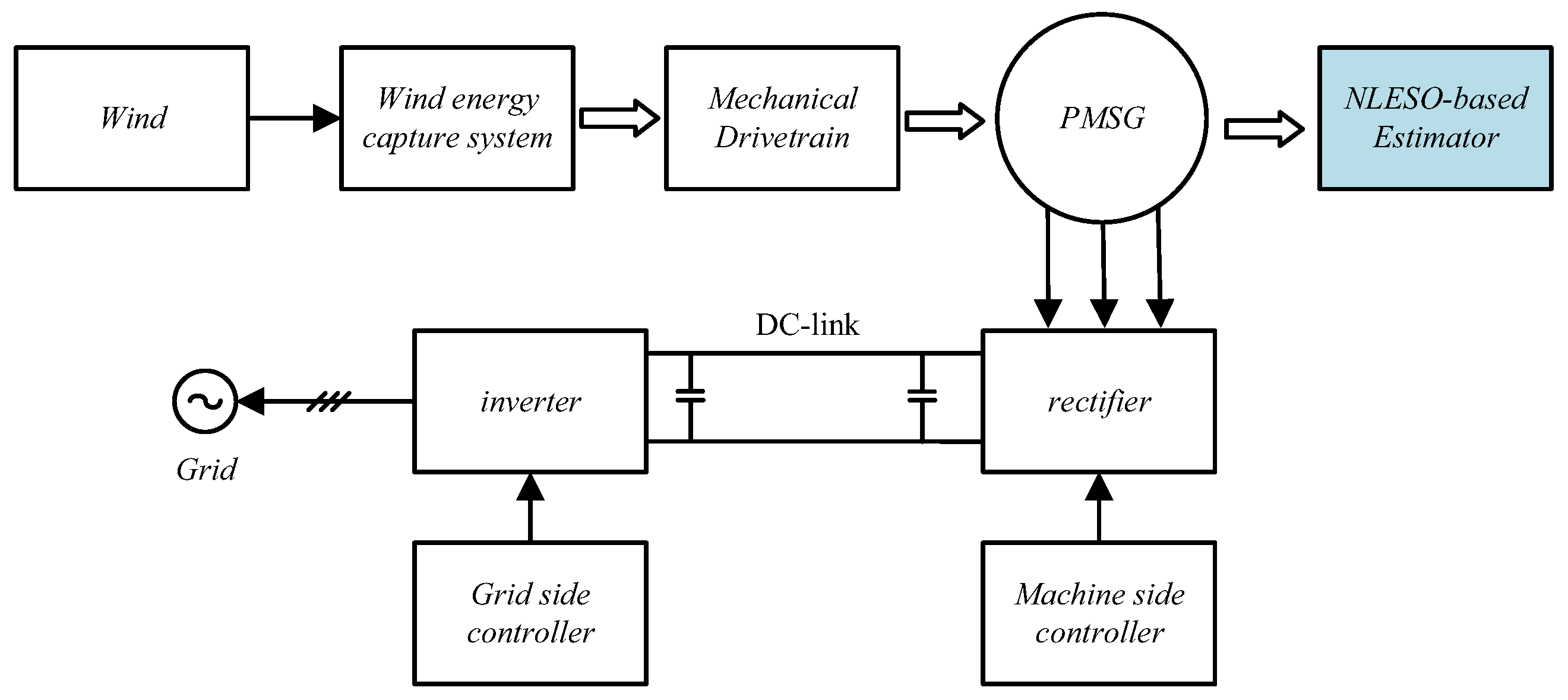
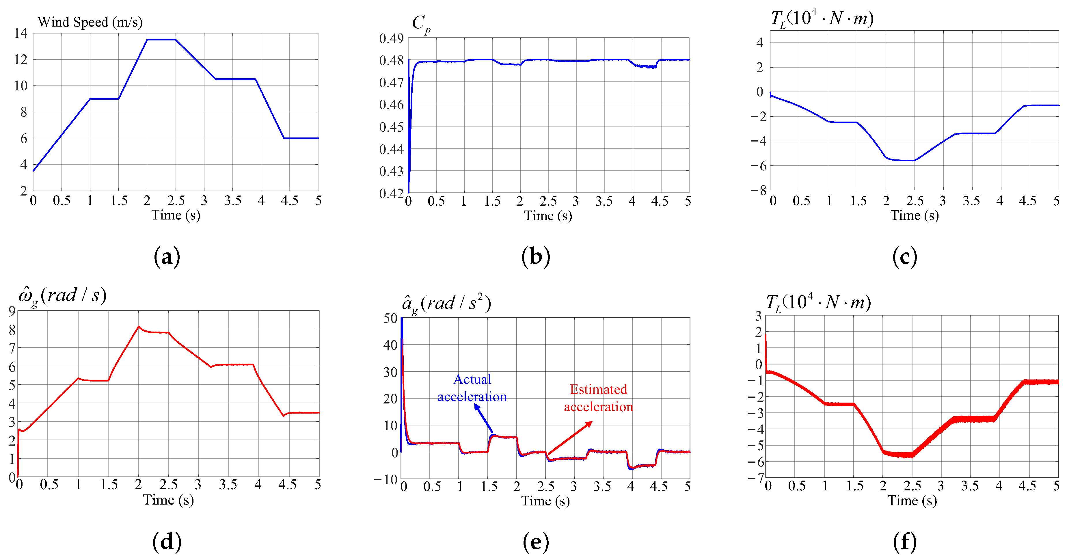
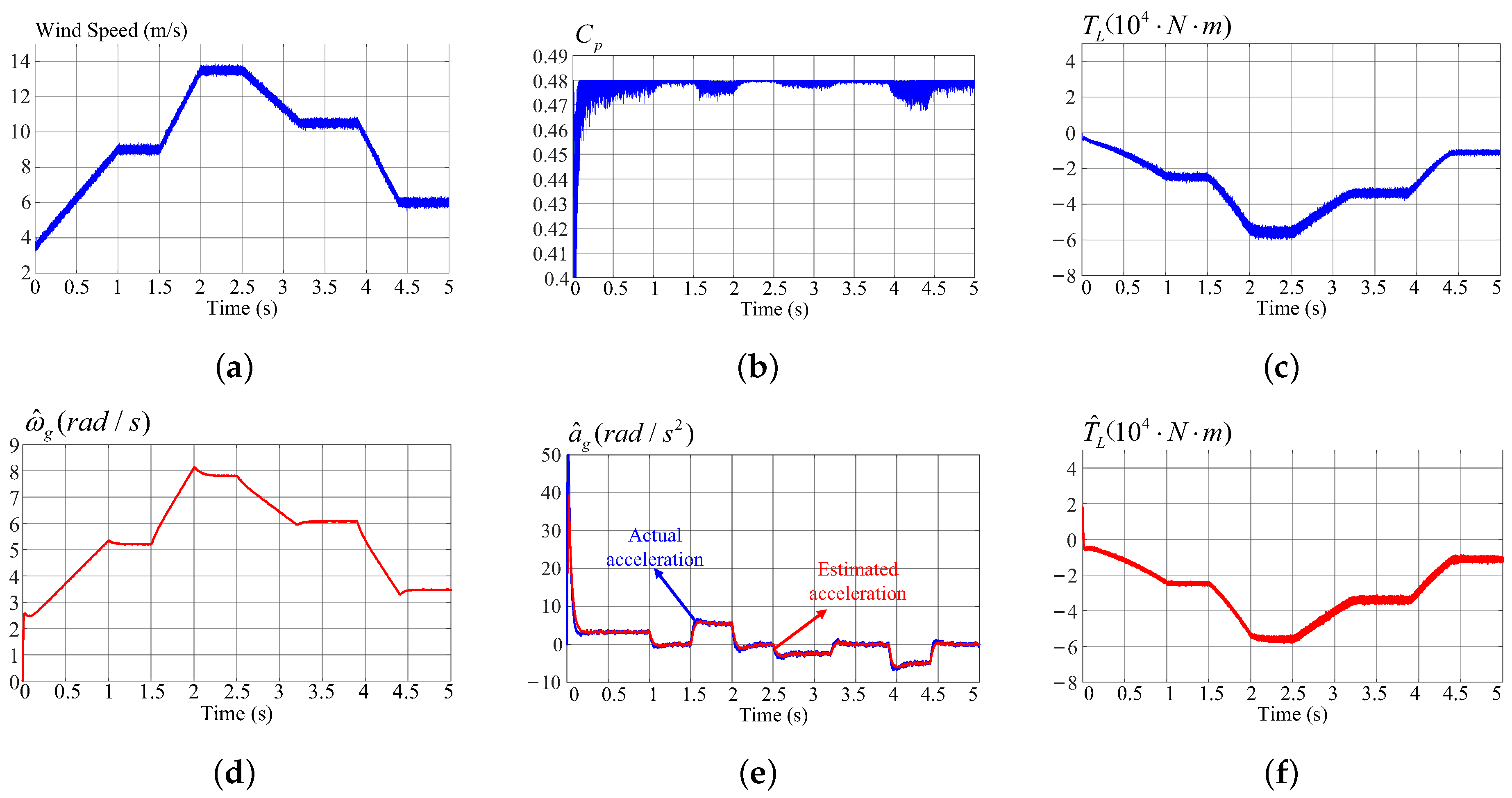
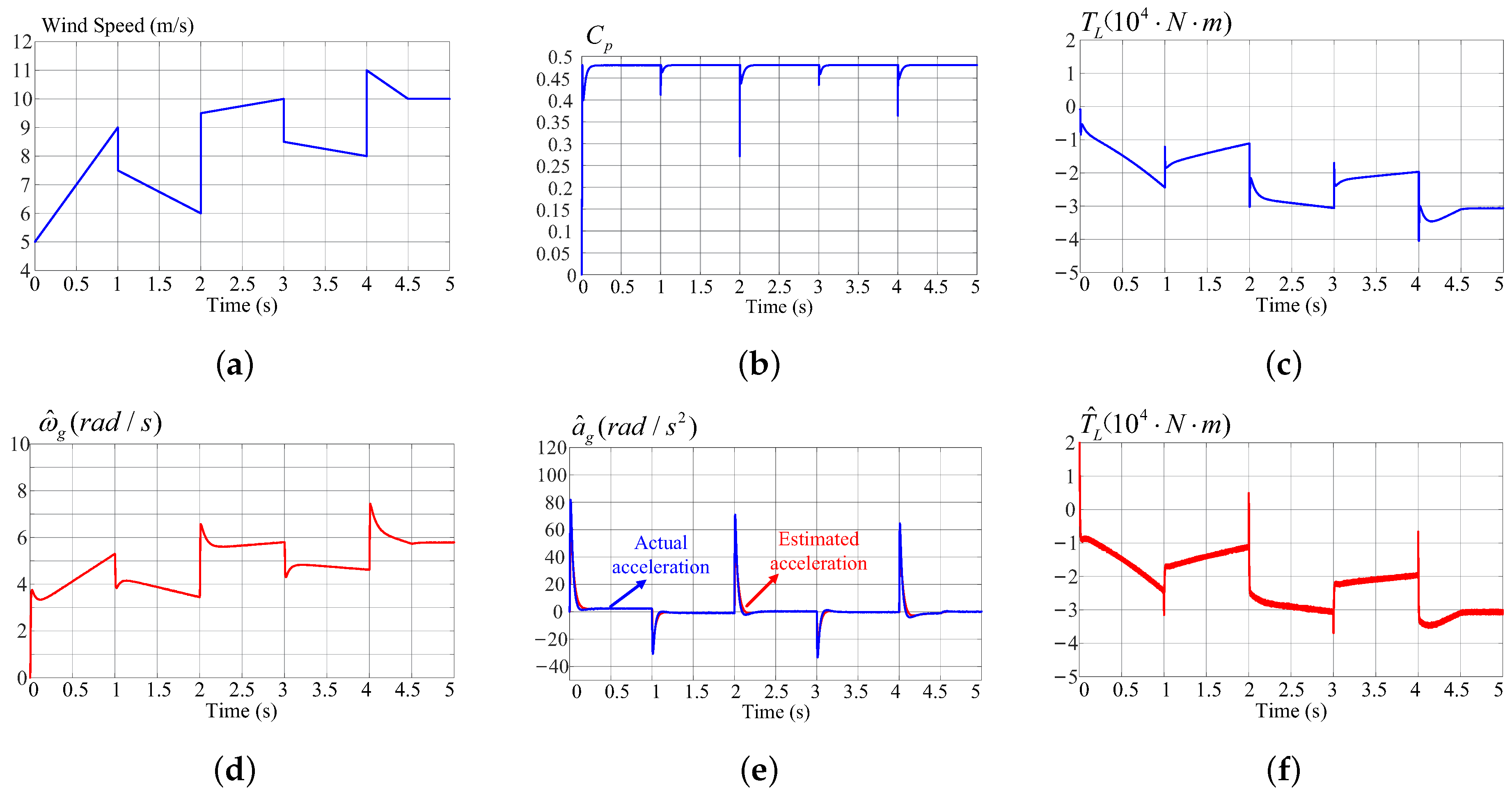
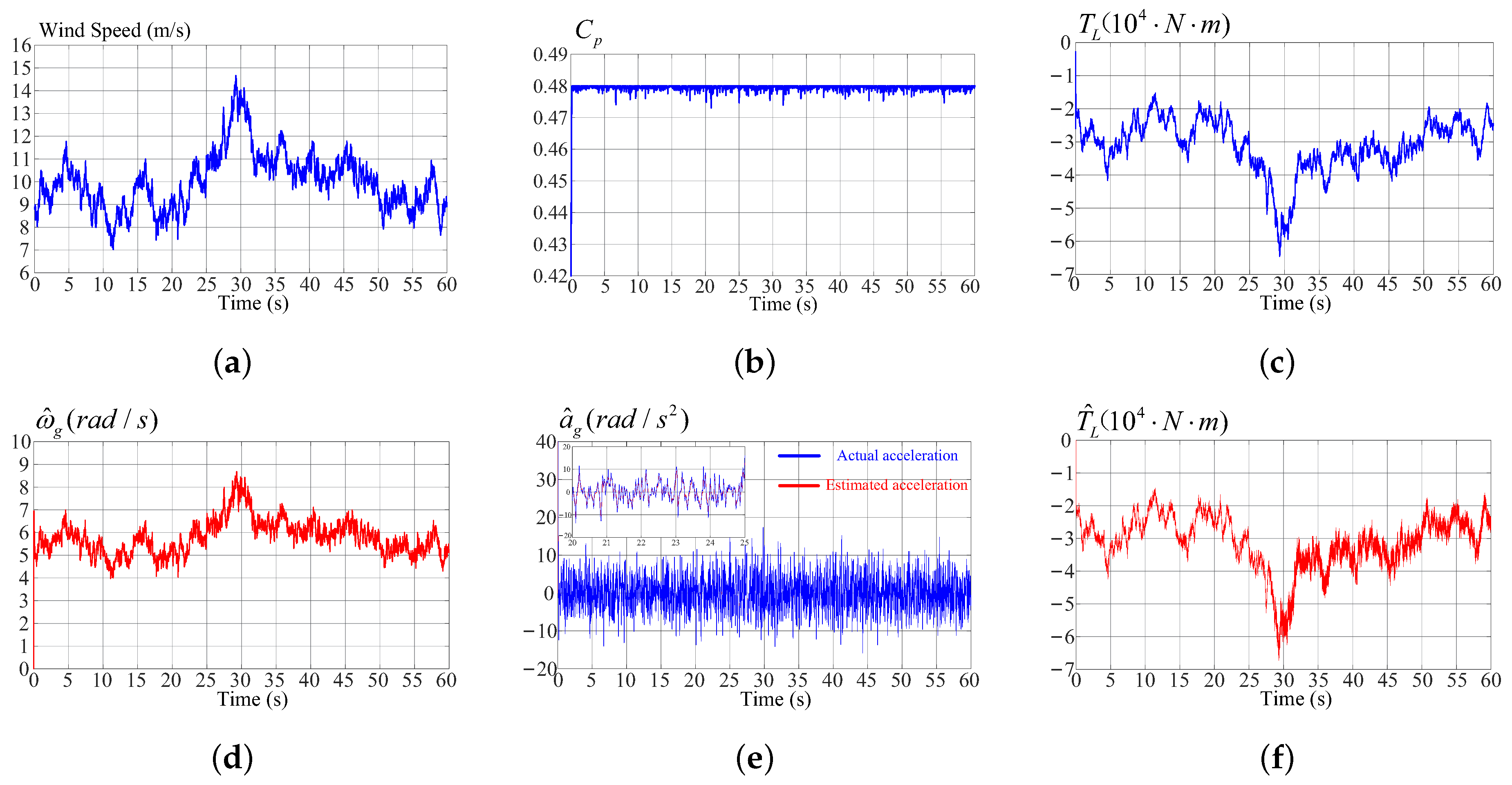
In this section, a PMSG simulation model based on Matlab/Simulink (MATLAB version: 9.14.0.2891782 (R2023a) Update 8) is built to verify the effectiveness of the proposed method in this paper. The general structural configuration of the simulation model is illustrated in Figure 2. The parameters used in simulations are given in

Table 1. Simulation model parameter.

Parameter	Description	Value
P	rated power	$300\mathrm{kW}$
J	Inertia	60 kg·m2
$n_p$	number of pole pairs	12
${\psi }_f$	permanent magnet flux linkage	$3.88889\mathrm{Wb}$
R	PMSG resistance	0.025 $\Omega$
L	PMSG inductance	$0.0036\mathrm{H}$

. In addition, the NLESO parameters are designed as ${\alpha }_1=0.5$, ${\delta }_1=0.01$, ${\beta }_1=700$, ${\alpha }_2=0.35$, ${\delta }_2=0.01$, ${\beta }_2$ = 20,000, ${\alpha }_3=1$, ${\delta }_3=0.01$, and ${\beta }_1$ = 800,000. To effectively demonstrate the previous theoretical analysis, the five different test conditions are adopted, as summarized in

Table 2. Simulation test conditions.

Cases	Test Conditions
Case A	Wind speed with gradual variation
Case B	Continuously varying wind speed
Case C	sinusoidally varying wind speed profile
Case D	Wind speed with gradual variation along with a 10% change of the stator resistance and inductance in the PMSG
Case E	Wind speed with gradual variation with superimposed wind speed noise
Case F	Wind speed with step change
Case G	Mean wind speed 10 m/s and turbulence intensity 0.14

. The corresponding simulation results are shown in the following sections.

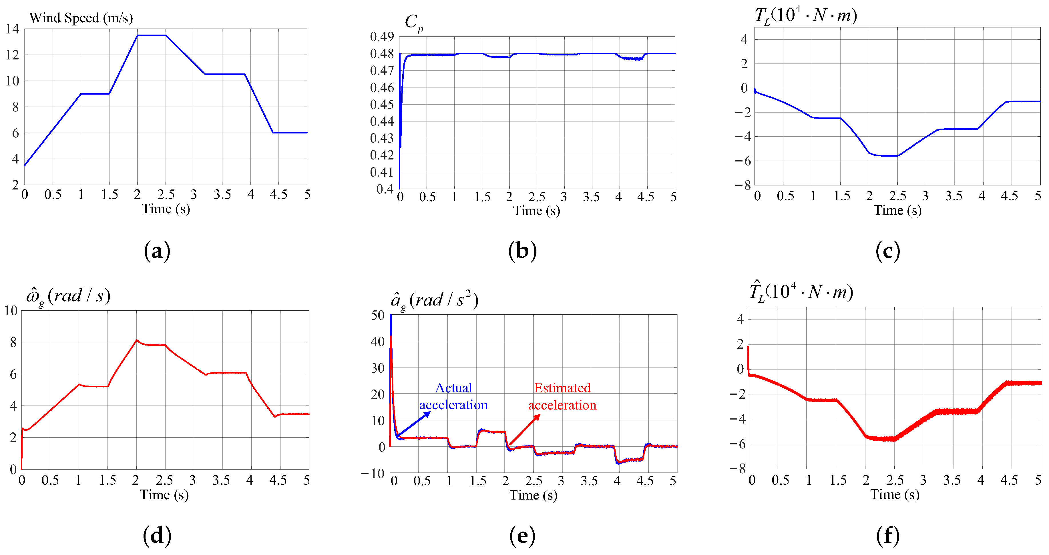
Case A: Under the scenario of case A, the wind speed exhibits a stepwise increase and decrease. Figure 3a illustrates this staged variation. Figure 3b shows the corresponding power coefficient ($C_p$), which reflects the efficiency of wind energy conversion. It is noteworthy that, despite the varying wind speed, the power coefficient is maintained near its optimal value. Figure 3c presents the actual load torque of the wind turbine, which changes correspondingly with the wind speed steps. Figure 3d illustrates the estimated rotational speed of the PMSG. Figure 3e displays both the estimated acceleration and the actual value (obtained by differentiating the measured speed and then applying a low-pass filter with a cutoff frequency of 30 rad/s). This result demonstrates that the estimated acceleration closely follows the dynamic behavior of the system. Figure 3f shows the estimated load torque of the wind turbine, which aligns well with the actual torque shown in Figure 3c. These results demonstrate that the proposed method can accurately and promptly track the load torque and other key dynamic parameters. Overall, the method exhibits excellent accuracy and responsiveness under the varying wind conditions of case A.

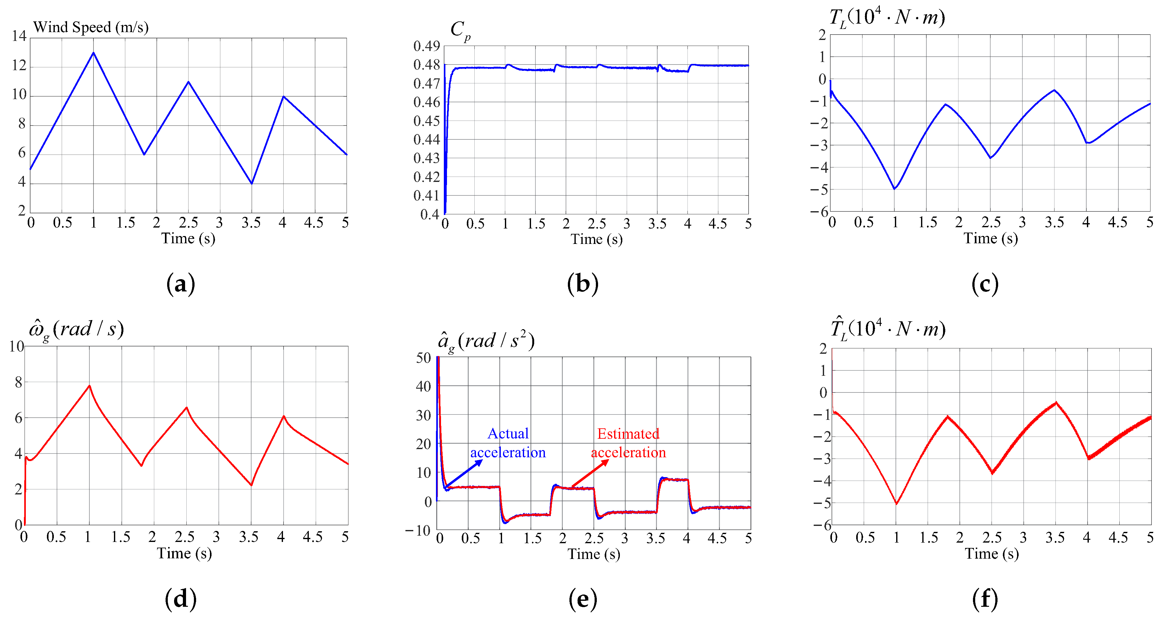
Case B: Under continuously varying wind speed conditions, the system experiences a more dynamic operating scenario. Figure 4a shows the continuous variation in wind speed over time. As illustrated in Figure 4b, the power coefficient ($C_p$) remains consistently near its optimal value, indicating effective wind turbine control under continuous wind fluctuations. Figure 4c depicts the actual load torque of the wind turbine. Figure 4d,e, respectively, illustrate the estimated speed and acceleration of the PMSG. Figure 4f shows the estimated load torque, which closely aligns with the actual torque, validating the accuracy of the proposed estimation method. These findings verify the accuracy and effectiveness of the proposed method under continuously varying wind conditions.

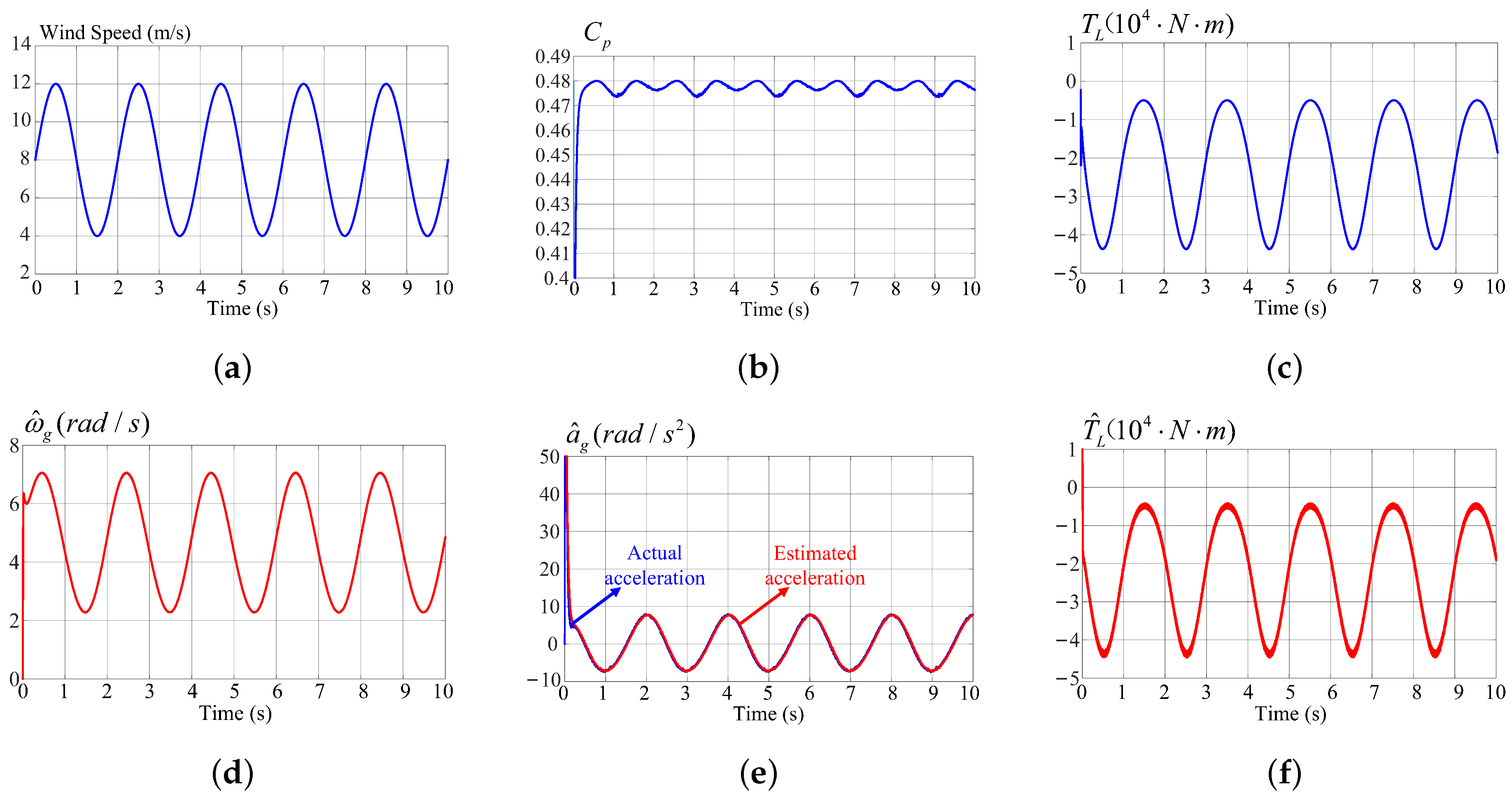
Case C: To further evaluate the performance of the proposed method under more complex operating conditions, a sinusoidally varying wind speed profile is introduced in this test case. Although such perfectly periodic wind variations rarely occur in real wind fields, this setting provides a stringent scenario for dynamic testing. As shown in Figure 5a, the wind speed fluctuates sinusoidally over time. Figure 5b presents the resulting power coefficient ($C_p$), which remains relatively stable and close to its optimal value despite continuous changes in wind speed. Figure 5c illustrates the actual load torque of the wind turbine, which exhibits a periodic variation consistent with the wind input. The generator’s estimated speed and acceleration are shown in Figure 5d,e, respectively. Both results closely follow the expected system dynamics. Figure 5f shows the estimated load torque, which exhibits high consistency with the actual torque curve in Figure 5c, confirming the method’s accuracy in torque estimation. These results indicate that the proposed method remains robust and precise even under continuous and cyclic wind disturbances.

Case D: Under the scenario of case D, the wind speed exhibits a gradual variation, accompanied by a 10% modification of the stator resistance and inductance in the PMSG. Although the parameter variations introduce only slight errors, the estimated load torque still closely follows the actual value, demonstrating the robustness of the proposed method. As shown in Figure 6a–f, the estimated rotational speed and acceleration also track the true system dynamics with high accuracy, while the power coefficient remains close to its optimal value. These results confirm that the proposed method can maintain reliable estimation performance even under parameter uncertainties.

Case E: Under this scenario, to account for the strong randomness inherent in real wind conditions, Gaussian white noise with a power of 0.1 W was superimposed on the gradually varying wind speed to emulate realistic fluctuations. As illustrated in Figure 7a–f, the wind speed input exhibits noticeable noise, causing fluctuations in the power coefficient and actual load torque. Nevertheless, the coefficient remains near its optimal value, and the estimated rotational speed, acceleration, and load torque still closely follow the actual values. These results demonstrate the robustness of the proposed method under noisy wind conditions.

Case F: To assess the proposed method’s performance under step disturbances, the wind speed was subjected to a sudden jump. As illustrated in Figure 8a–f, although the step disturbance introduced abrupt changes, the estimated variables rapidly reached a steady state, demonstrating the robustness of the method. After stabilization, the estimation errors for acceleration and load torque remained small and closely tracked the actual values. These results indicate that the proposed approach can provide accurate and reliable estimation even in the presence of sudden wind variations.

Case G: To better reflect realistic operating conditions, the mean wind speed was set to 10 m/s with a turbulence intensity of 0.14, and the simulation time was 60 s. Figure 9a illustrates the wind speed profile with turbulence, while Figure 9b,c show the corresponding power coefficient and actual torque, respectively. Due to the influence of turbulence, fluctuations appear in the turbine’s rotational speed and acceleration. Nevertheless, the estimated acceleration and load torque are still able to closely follow their actual values, demonstrating the effectiveness of the proposed method under turbulent wind conditions.

4. Conclusions

In this paper, a nonlinear extended state observer-based method was proposed for the estimation of rotational speed and generator load torque in a PMSG wind turbine. Unlike conventional approaches that rely on torque sensors, the proposed method utilizes only current and acceleration information, thereby enhancing system reliability and reducing hardware costs. These estimated parameters are of critical importance for ensuring stable operation, improving fault tolerance, and supporting advanced control strategies in wind energy conversion systems. Theoretical analysis was conducted to rigorously guarantee the stability of the proposed estimation scheme. Furthermore, simulation studies under different wind scenarios—including stepwise, continuous, and sinusoidal wind variations—were carried out to validate the effectiveness and robustness of the method. However, the current work is mainly limited to theoretical analysis and simulation studies, with a lack of experimental validation. Therefore, future research will focus on investigating the feasibility of the proposed method in real wind farm environments.

References

1. Rahideh, A.; Korakianitis, T. Analytical magnetic field distribution of slotless brushless machines with inset permanent magnets. IEEE Trans. Magn. 2011, 47, 1763–1774. [Google Scholar] [CrossRef]
2. Pastore, L.M.; Basso, G.L.; Ricciardi, G.; de Santoli, L. Synergies between Power-to-Heat and Power-to-Gas in renewable energy communities. Renew. Energy 2022, 198, 1383–1397. [Google Scholar] [CrossRef]
3. Aissou, R.; Rekioua, T.; Rekioua, D.; Tounzi, A. Application of nonlinear predictive control for charging the battery using wind energy with permanent magnet synchronous generator. Int. J. Hydrogen Energy 2016, 41, 20964–20973. [Google Scholar] [CrossRef]
4. Wang, Y.; Hu, Q.; Li, L.; Foley, A.M.; Srinivasan, D. Approaches to wind power curve modeling: A review and discussion. Renew. Sustain. Energy Rev. 2019, 116, 109422. [Google Scholar] [CrossRef]
5. Wang, Y.; Cai, X.; Wu, A.; Xu, B.; Lin, S. Turbulence intensity identification and load reduction of wind turbine under extreme turbulence. Ocean. Eng. 2022, 257, 111710. [Google Scholar] [CrossRef]
6. Mérigaud, A.; Ringwood, J.V. Condition-based maintenance methods for marine renewable energy. Renew. Sustain. Energy Rev. 2016, 66, 53–78. [Google Scholar] [CrossRef]
7. Liu, W.; Tang, B.; Han, J.; Lu, X.; Hu, N.; He, Z. The structure healthy condition monitoring and fault diagnosis methods in wind turbines: A review. Renew. Sustain. Energy Rev. 2015, 44, 466–472. [Google Scholar] [CrossRef]
8. Salameh, J.P.; Cauet, S.; Etien, E.; Sakout, A.; Rambault, L. Gearbox condition monitoring in wind turbines: A review. Mech. Syst. Signal Process. 2018, 111, 251–264. [Google Scholar] [CrossRef]
9. Valikhani, M.; Jahangiri, V.; Ebrahimian, H.; Moaveni, B.; Liberatore, S.; Hines, E. Inverse modeling of wind turbine drivetrain from numerical data using Bayesian inference. Renew. Sustain. Energy Rev. 2023, 171, 113007. [Google Scholar] [CrossRef]
10. Hosseini, A.; Cannon, D.T.; Vasel-Be-Hagh, A. Wind farm active wake control via concurrent yaw and tip-speed ratio optimization. Appl. Energy 2025, 377, 124625. [Google Scholar] [CrossRef]
11. Hosseini, A.; Cannon, D.T.; Vasel-Be-Hagh, A. Tip speed ratio optimization: More energy production with reduced rotor speed. Wind 2022, 2, 691–711. [Google Scholar] [CrossRef]
12. Kamel, O.; Hauptmann, S.; Bottasso, C. Estimation of damage equivalent loads of Drivetrain of wind turbines using machine learning. J. Phys. Conf. Ser. 2022, 2265, 032075. [Google Scholar] [CrossRef]
13. Yoon, Y.D.; Sul, S.K.; Morimoto, S.; Ide, K. High-bandwidth sensorless algorithm for AC machines based on square-wave-type voltage injection. IEEE Trans. Ind. Appl. 2011, 47, 1361–1370. [Google Scholar] [CrossRef]
14. Wang, D.; Li, B.; Zhao, Y. An Adaptive SMO Approach for Low-Chattering Sensorless Control of PMSM. IEEE Trans. Power Electron. 2025, 2, 1–9. [Google Scholar] [CrossRef]
15. Lee, J.; Hong, J.; Nam, K.; Ortega, R.; Praly, L.; Astolfi, A. Sensorless control of surface-mount permanent-magnet synchronous motors based on a nonlinear observer. IEEE Trans. Power Electron. 2009, 25, 290–297. [Google Scholar]
16. Cooperman, A.; Martinez, M. Load monitoring for active control of wind turbines. Renew. Sustain. Energy Rev. 2015, 41, 189–201. [Google Scholar] [CrossRef]
17. Liu, X.; Bo, L.; Luo, H. Dynamical measurement system for wind turbine fatigue load. Renew. Energy 2016, 86, 909–921. [Google Scholar] [CrossRef]
18. Gambier, A.; Nazaruddin, Y.Y. Modelling the wind turbine by using the tip-speed ratio for estimation and control. Energies 2022, 15, 9454. [Google Scholar] [CrossRef]
19. Tautz-Weinert, J.; Watson, S.J. Using SCADA data for wind turbine condition monitoring—A review. IET Renew. Power Gener. 2017, 11, 382–394. [Google Scholar] [CrossRef]
20. Lee, S.; Churchfield, M.; Driscoll, F.; Sirnivas, S.; Jonkman, J.; Moriarty, P.; Skaare, B.; Nielsen, F.G.; Byklum, E. Load estimation of offshore wind turbines. Energies 2018, 11, 1895. [Google Scholar] [CrossRef]
21. Loriemi, A.; Jacobs, G.; Bosse, D. Estimation of rotor and main bearing loads using artificial neural networks. J. Phys. 2022, 2151, 012002. [Google Scholar] [CrossRef]
22. Klein, A.; Wintermeyer-Kallen, T.; Stegink, J.; Kösters, T.; Zierath, J.; Nelles, O.; Abel, D.; Vallery, H.; Basler, M. Control-oriented wind turbine load estimation based on local linear neuro-fuzzy models. J. Phys. Conf. Ser. 2024, 2767, 032016. [Google Scholar] [CrossRef]
23. Meng, L.; Zhu, Y.; Xu, S.; Xu, S.; Yang, K. Torque Estimation Based on An Improved SOGI-FLL for IPMSM. In Proceedings of the 2024 IEEE International Conference on Mechatronics and Automation (ICMA), Tianjin, China, 4–7 August 2024; pp. 1188–1193. [Google Scholar]
24. Zhang, Y.; Yin, Z.; Tang, R.; Liu, J. Moment of Inertia and Load Torque Identification Based on Adaptive Extended Kalman Filter for Interior Permanent Magnet Synchronous Motors. IEEE Trans. Instrum. Meas. 2025, 74, 1–12. [Google Scholar] [CrossRef]
25. Mohamed, Y.A.R.I. A Newly Designed Instantaneous-Torque Control of Direct-Drive PMSM Servo Actuator With Improved Torque Estimation and Control Characteristics. IEEE Trans. Ind. Electron. 2007, 54, 2864–2873. [Google Scholar] [CrossRef]
26. Liu, L.; Song, H.; Liang, D. High Performance Sensorless Control of PMSM with Sliding Mode Load Torque Observer. In Proceedings of the 2020 4th International Conference on HVDC (HVDC), Xi’an, China, 6–9 November 2020; pp. 1060–1065. [Google Scholar]
27. Wu, Z.; Wang, X.; Ren, N.; Li, G.; Dai, Z. An acceleration-observer-based position and load torque estimation method for wind turbine with sensor faults. Energies 2025, 18, 2787. [Google Scholar] [CrossRef]
28. Watil, A.; El Magri, A.; Raihani, A.; Lajouad, R.; Giri, F. An adaptive nonlinear observer for sensorless wind energy conversion system with PMSG. Control. Eng. Pract. 2020, 98, 104356. [Google Scholar] [CrossRef]
29. Niu, L.; Xu, D.; Yang, M.; Gui, X.; Liu, Z. On-line Inertia Identification Algorithm for PI Parameters Optimization in Speed Loop. IEEE Trans. Power Electron. 2015, 30, 849–859. [Google Scholar] [CrossRef]
30. Beller, S. Torque estimation with artificial intelligence methods in a brushed geared DC motor. Çukurova Üniv. Mühendis. Fak. Derg. 2022, 37, 885–898. [Google Scholar] [CrossRef]
31. Lončarek, T.; Lešić, V.; Vašak, M. Increasing accuracy of Kalman filter-based sensorless control of wind turbine PM synchronous generator. In Proceedings of the 2015 IEEE International Conference on Industrial Technology (ICIT), Seville, Spain, 17–19 March 2015; pp. 745–750. [Google Scholar]
32. Zhao, Y.; Li, G.; Dai, Z.; Li, B.; Lin, H.; Yang, J. Integral-type half-tangent phase-locked loop for more electric aircraft grids. IET Power Electron. 2023, 16, 1472–1485. [Google Scholar] [CrossRef]
Figure 1. Control structure of the proposed NLESO-based load torque estimator.
Eng 06 00264 g001
Figure 2. General structure of the wind generation system simulation model.
Eng 06 00264 g002
Figure 3. Simulation results under case A. (a) Target wind speed variation. (b) Power coefficient of the wind turbine ( C p ). (c) Actual load torque of the wind turbine. (d) Estimated speed of the PMSG. (e) Estimated acceleration of the PMSG. (f) Estimated load torque of the wind turbine.
Eng 06 00264 g003
Figure 4. Simulation results under case B. (a) Target wind speed variation. (b) Power coefficient of the wind turbine ( C p ). (c) Actual load torque of the wind turbine. (d) Estimated speed of the PMSG. (e) Estimated acceleration of the PMSG. (f) Estimated load torque of the wind turbine.
Eng 06 00264 g004
Figure 5. Simulation results under case C. (a) Target wind speed variation. (b) Power coefficient of the wind turbine ( C p ). (c) Actual load torque of the wind turbine. (d) Estimated speed of the PMSG. (e) Estimated acceleration of the PMSG. (f) Estimated load torque of the wind turbine.
Eng 06 00264 g005
Figure 6. Simulation results under case D. (a) Target wind speed variation. (b) Power coefficient of the wind turbine ( C p ). (c) Actual load torque of the wind turbine. (d) Estimated speed of the PMSG. (e) Estimated acceleration of the PMSG. (f) Estimated load torque of the wind turbine.
Eng 06 00264 g006
Figure 7. Simulation results under case E. (a) Target wind speed variation. (b) Power coefficient of the wind turbine ( C p ). (c) Actual load torque of the wind turbine. (d) Estimated speed of the PMSG. (e) Estimated acceleration of the PMSG. (f) Estimated load torque of the wind turbine.
Eng 06 00264 g007
Figure 8. Simulation results under case F. (a) Target wind speed variation. (b) Power coefficient of the wind turbine ( C p ). (c) Actual load torque of the wind turbine. (d) Estimated speed of the PMSG. (e) Estimated acceleration of the PMSG. (f) Estimated load torque of the wind turbine.
Eng 06 00264 g008
Figure 9. Simulation results under case G. (a) Target wind speed variation. (b) Power coefficient of the wind turbine ( C p ). (c) Actual load torque of the wind turbine. (d) Estimated speed of the PMSG. (e) Estimated acceleration of the PMSG. (f) Estimated load torque of the wind turbine.
Eng 06 00264 g009