Abstract
The problem addressed in this article consists of the motion control of a quadrotor affected by model disturbances and uncertainties. In order to tackle model uncertainty, adaptive control based on reinforcement learning is used. The distinctive feature of this article, in comparison with other works on quadrotor control using reinforcement learning, is the exploration of the underlying optimal control problem in which a quadratic cost and a linear dynamics allow for an algorithm that runs in real time. Instead of identifying a plant model, adaptation is obtained by approximating the performance index given by the Q-function using directional forgetting recursive least squares that rely on a linear regressor built from quadratic functions of input/output data. The adaptive algorithm proposed is tested in simulation in a cascade control structure that drives a quadrotor. Simulations show the improvement in performance that results when the proposed algorithm is turned on.
1. Introduction
1.1. Motivation
Unmanned aerial vehicles are currently becoming an important player in areas such as inspection and maintenance, photography, surveillance, mapping, agriculture, military warfare, delivery, and more [1,2]. Fully automated vehicles without human intervention have been receiving increased attention [3], as advanced controller architectures are [1,2] progressing towards full autonomy, an example of which includes adaptive controllers that can tackle wind perturbations or uncertainty in the model parameters.
Reinforcement learning (RL) is a technique in which the control action that is applied to the manipulated variable of the plant is selected so as to maximize a reward signal [4]. Some RL algorithms can provide adaptation without the need for model knowledge about the system upon which it acts. This opens a gateway for a new class of adaptive controllers that can attain some degree of control robustness. The topic of drone control using RL has been the subject of many recent works. In addition to the works reviewed in [2], other references include [5,6,7], as well as [8,9], that address real-time RL.
Although general RL-based controllers yield remarkable performances for a wide variety of robotic and aircraft plants [10], the fact that they rely on deep neural networks implies long training periods, with a massive computational load, that may only be executed off-line. Nevertheless, for a class of problems in which the plant dynamics is linear and the cost to optimize is quadratic, the computational load is greatly reduced, being compatible with on-line adaptive control.
This work has the objective of developing an adaptive controller for a quadrotor based on a specific RL model-free algorithm, along the lines presented in [11]. It is stressed that, contrary to the works reported in [2], the algorithm proposed in this article does not rely on off-line training using massive amounts of data but, instead, provides real-time adaptation of a vector of state feedback gains, without knowing or estimating the parameters of any plant model. By real-time adaptation, it is meant that the algorithm is fast enough to be run as the drone operates. This procedure is possible because we restrain the class of problems addressed to be of the linear quadratic type, i.e., defined by an underlying plant dynamics to be linear but unknown and a quadratic performance cost to be minimized.
Assuming the underlying plant dynamics to be linear is justified by the type of application envisaged: the algorithm developed is embedded in the control part of the quadrotor GNC (guidance, navigation, and control) system and has the task of regulating the quadrotor state around a reference trajectory generated by the guidance system. Hence, the controller is required to tackle only incremental dynamics that may be approximated by a linear model.
With respect to other works described in the literature for motion control of quadrotors based on reinforcement learning [2], the approach proposed here has the drawback of not allowing large amplitude maneuvers, in which the nonlinear character of the dynamics dominates. In compensation, the control algorithm proposed provides a model-free adaptive controller that operates in real time with little a priori plant knowledge. The design and use of such a controller for drone motion is the focus of this article.
1.2. Problem Definition, Objectives, and Contribution
A common control architecture for quadrotors consists of two controllers interconnected in a cascade structure: an outer control loop, responsible for keeping the quadrotor in a desired position, and an inner control loop that tracks the quadrotor attitude demanded by the outer controller.
The attitude controller works on the premise that the quadrotor is not performing extreme maneuvers, so it is valid to assume that the drone dynamics is approximately linear. In order to tackle uncertainty in dynamics, the inner loop that regulates the attitude relies on an adaptive controller that embeds a reinforcement learning (RL) algorithm to learn the gains that optimize a quadratic cost.
The outer loop consists of a linear quadratic (LQ) controller with constant gains, designed using a nominal model, and it has a time scale that is much slower than the one of the inner loop.
The contribution of this article consists of the design of the above cascade adaptive control architecture and its demonstration in simulations for a quadrotor model. The main innovative feature is the embedding of a reinforcement learning algorithm in the inner loop to yield a model-free adaptive controller. The use of a directional forgetting least-squares estimation algorithm to avoid identifiability problems in the Q-function approximator is a contribution.
2. Dynamics Modeling
Although the proposed controller does not rely on a model, the dynamics of the drone considered is described in this section for the purposes of simulation and interpretation of the results presented later.
The model dynamics follows the rigid body equations of motion [12]. In this case, an inertial reference frame attached to the ground and a fixed body frame attached to the vehicle are defined as represented in Figure 1.
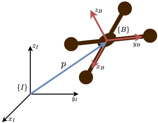
Figure 1.
Quadrotor with inertial reference frame and fixed body frame defined.
The rigid body state comprises a position in the inertial frame p, a velocity in the body frame v, an angular velocity in the body frame , and a rotation matrix R that represents the transformation between the fixed body frame and the inertial frame orientations. The full kinematics equations are:
where the quadrotor attitude is expressed in Euler angles, a vector with the elements as the angle of rotation about the x axis, as the angle of rotation about the y axis, and as the angle of rotation about the z axis. The matrix Q is defined as
The dynamics equations are
where J represents the moment of inertia matrix, which is assumed to be diagonal. The application corresponds to a skew-symmetric matrix. The inputs T and n represent the thrust force and torque, respectively.
3. Controlling the Quadrotor
3.1. Controller Structure
The relationship between both sets of Equations (1) and (3) allows for the development of a cascade control structure that has an inner loop for controlling the attitude of the quadrotor and an outer loop for controlling the position and that generates as a manipulated variable the desired orientation to the inner (attitude) controller. This type of controller is commonly used in UAVs, and its block diagram is shown in Figure 2.
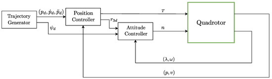
Figure 2.
Cascade controller for the quadrotor motion.
The trajectory generator block creates the references , , and for the position controller and the reference for the attitude controller. These signals represent the desired position and its derivatives and the desired angle, respectively. Besides generating an input thrust T, the position controller also generates a desired upwards orientation corresponding to the third column of R, which is combined with in the attitude controller to track the desired orientation angles.
3.2. Position Controller
Neglecting the rotational dynamics, it is assumed that the desired orientation, , can be forced upon the system. Considering that , the virtual input is defined and transforms the first line of (3) into
which is now a linear system that can be controlled with a linear controller.
For the sake of reference trajectory tracking, define the tracking error e by
where represents the reference position yielded by the guidance subsystem. Taking the second derivative of (5) and resorting to (4), the error dynamics
is obtained. Selecting the virtual control variable to be
introduces linear state feedback, where each state has a proportional gain. There is also a correction term in order to eliminate the second derivative of the error present in the dynamics. Applying the control law (7) transforms (6) into
where the gains and are selected so as to drive the error e to zero, enabling reference tracking of a desired trajectory with time derivatives and .
The virtual control input , which is a three-dimensional vector, is translated into the thrust T input and the desired orientation (forced upon the system) values. Via Equation (7), the thrust T is calculated with
and the desired orientation is obtained through
The thrust input is fed directly into the system, as opposed to , which is passed to the attitude controller so that the orientation errors can also be regulated.
3.3. Attitude Controller
Neglecting the translational dynamics, the desired orientation is fed to the attitude controller, which produces, as manipulated variable, an input torque for the system.
To track the desired orientation value, the desired angle, , is combined with to obtain the remaining desired angles and .
Through decomposition of the desired R matrix, the equation
allows the computation of the desired attitude . To track this value, a possible strategy is to linearize the second equations of systems (1) and (3) around the hover condition, a valid approach for smooth trajectories where aggressive maneuvers are not required, resulting in
given that the matrix J is diagonal. The linearized system obtained is also a double integrator. The input n is chosen to account for the angle and angular velocity error, resulting in
The inner loop that comprises the attitude controller must react faster than the outer loop containing the position controller. This time scale separation is forced to ensure that the system quickly corrects angle displacements that are detrimental to effectively tracking the desired position. To guarantee correctness, the gains of each controller must be chosen such that the inner loop poles contain a real part that is 10 times (or more) larger than the real part of the outer loop poles.
3.4. Underlying LQ Control
The adaptive RL controller proposed in this article consists of a state feedback in which the gains converge to those of an LQ controller. Hereafter, the model and the quadratic cost that define this underlying controller are defined. Assuming that the inputs are piece-wise constant over the sampling period h, the discrete-time equivalent [13] of the double integrator dynamics takes the form , with
and where, for the case of the rotational dynamics, is the diagonal element from the inertial moment matrix J associated with the angle to be controlled. For the case of the translational dynamics, the mass scaling is incorporated in the virtual input , and thus .
Having both and , the discrete controller gains for the control laws in (7) and (13) can be calculated resorting to the LQR algorithm, which aims at minimizing the quadratic cost
A careful choice of the and weight matrices is necessary for good performance.
The sampling period selected throughout all experiences is , equivalent to a frequency of 100 Hz. The quadrotor state variables are assumed to be fully observable. Sensor noise is modeled by adding white noise after the A/D sampling process. A standard deviation of (with zero mean) is used in the simulation.
4. Reinforcement Learning
4.1. Introduction
Reinforcement learning is an area of machine learning that aims to learn the best action an agent can execute as it interacts with the environment that it acts upon, such that a reward is optimized [4]. From a control perspective, we can think of the environment as the system and the action as the output produced by the controller, which is the agent [14].
In this setting, the action is now the control action , and the state is . The control policy determines the value of , and it is defined as
for a map from the state space to the control space. Since this map depends only on the current state , it defines a state feedback controller. This definition needs to be coherent with the definition of the reward signal, as detailed further below.
Hereafter, the system is described by
where A and b are matrices that define the linearized quadrotor dynamics.
4.2. Dynamic Programming and Q-Function
The control policy is to be designed such as to minimize
often called the cost-to-go or return. The discount factor takes values in the interval .
For the reward signal, this article considers the quadratic function
In order to obtain model-free controllers, define the Q-function
The Q-function verifies a Bellman-like equation given by
The optimal control policy is then calculated through
In the absence of constraints, the optimal control policy can then be computed by solving
4.3. Approximate Dynamic Programming
To determine the optimal policy at time k, it is necessary to know the optimal policy at time . This minimization process is done backwards in time, and it is only feasible as an off-line planning method using iterative algorithms [11]. The resulting dynamic programming methods are not enough to obtain a controller that is able to learn in real time. Approximate dynamic programming solves this problem and introduces two other concepts that will make the operation forward in time possible.
The first concept required is that of temporal difference (TD). Taking advantage of Equation (21), it is possible to define a residual error given by
If the Bellman equation is satisfied, then the error is zero. This error can be seen as the difference between observed and predicted performances when a previously calculated action is applied. The next important tool is the value function approximation (VFA), which approximates the Q-function by means of a parametric approximator. For linear plants and quadratic costs, it can be shown [11] that the Q-function can be rewritten as
where W is a vector of coefficients, and is a vector containing the basis functions with the square terms and cross terms for all elements of and .
Combining Equations (25) and (24), the TD error becomes
which defines a linear regression model with parameters W. Approximating by means of a linear combination of basis functions enables the use of estimation techniques to obtain the coefficients that will then define the closest approximation [11]. Equations (21), (22) and (25) allow for building an on-line forward-time learning algorithm for state feedback control.
4.4. Q-Learning Policy Iteration
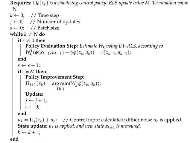
In this article, the policy iteration adapted for Q-learning is chosen to be applied in the controller.
The Policy Evaluation Step, where the VFA coefficients are estimated, requires determining a least squares solution to find the estimate of the parameter vector W in the linear regression model (26). This can be done by resorting to recursive least squares (RLS) or batch least squares. In this article, directional forgetting RLS [15] is used.
A Gaussian dither noise is added to the observed control input signal , derived from the current policy , obtained from (23). The reason behind this procedure is the necessity to ensure the persistence of an excitation condition. The absence of this effect can cause the algorithm to completely fail [11].
For estimation purposes, recursive least squares with directional exponential forgetting (DF-RLS) is used [15], where the estimated Q-function gains are updated at every time step k, and the policy is updated after a fixed number of time steps. Since a recursive version of least squares is used, the estimates are updated at each sampling time. The Q-learning algorithm using DF-RLS is detailed in Algorithm 1. The time step of executing Algorithm 1 is equal to the beginning of each sampling time.
For a two-dimensional state system, the VFA is defined as in (25), with the basis functions given by
which means that the policy improvement step at the update , as defined in Algorithm 1, takes the form
The control action takes the form of a linear state feedback , with a K gain of
where represents the estimate of the ith element of W.
| Algorithm 1: Q-Learning Policy Iteration, DF-RLS Update |
 |
The importance of the use of DF-RLS stems from the fact that, although there are only two controller gains, the Q-function is approximated by six parameters, a fact that may cause identifiability problems.
In adaptive control, the time scale of the action update, i.e., of the value of the manipulated variable, must be slower than that of the learning variable (in this case, learning the parameters that define the control action), in order to decouple the dynamics of learning from plant dynamics. In order to enhance this feature, the controller gains that define the control action are only recomputed at a lower rate (every M steps), even though the RLS parameters of the Q-function approximation are updated at every sampling rate (as well as the control action).
5. Simulation Study
This section presents simulations that illustrate the results obtained when applying the above algorithm to control the motion of the quadrotor model described in Section 2. The simulation experiments show that, with the proposed controller, the closed-loop system is able to track a reference in which there are curved sections followed by segments that are approximately straight. More important, the simulations illustrate adaptation. There is an initial period in which a constant vector of a priori chosen controller gains is used. During this period, the algorithm is learning the optimal gains, but these estimates are not used for feedback. After this initial period, the gains learned by the RL algorithm are used.
There are two sets of experiments. In the first set, the initial gains are far from the optimum. In the second set of experiments, the initial set of gains is not optimal, but closer to optimum than the gains in the first set. Two relevant results are shown: one is the ability of the algorithm to improve the performance when the gains obtained by RL are used; furthermore, the dither noise can be reduced when the initial gains are closer to the optimum (that is to say, when more a priori information is available). The evaluation and comparison of the different situations is done using an objective index (the “score”) defined below.
Usually, control action decisions based on RL are obtained by training neural networks, requiring very large amounts of plant input/output data and, therefore, taking a long time before convergence. However, in the approach followed in this article, the approximation of the Q-function does not rely on neural network training but, instead, on recursive least-squares that have a fast convergence rate. Again, this feature is rendered possible by the class of control problems (linear-quadratic) considered.
The wind force w is characterized by its x, y, and z components, which determine its direction and magnitude. White noise is applied to a low-pass filter and added to w to produce more realistic deviations from the average magnitude. The average value of the disturbance is assumed to be measurable and is compensated for, but the model is still affected by the white noise effect, which has a standard deviation of . The wind disturbance value for the i component is described as
where represents the generated wind, represents the average value, and represents the filtered white noise. The dynamics of the motor are neglected, being considered much faster than the remaining quadrotor dynamics. The aerodynamic drag effect is also neglected, since most of the quadrotor operations are maintained in a near-hover condition.
The model considered has the following parameters:
- •
- Kg;
- •
- m;
- •
- Kg·m2;
- •
- Kg·m2.
For simulation purposes, the constant wind disturbance is compensated, assuming that it is possible to measure its average value. The noisy oscillations around the average value still affect the system.
To gain a better insight into how well the controller performs before and after the learning process, a performance metric is defined as
where represents the desired position and p the actual position. The metric calculates the average value of the distance between the moving point in the reference trajectory and the actual position of the quadrotor. The lower this value, the better the controller can track the given reference trajectory.
The control algorithm parameters are selected by trial and error in simulations. The main parameters to adjust are the weights in the quadratic cost considered and the dither noise variance added to the control variable. The dither noise variance must be chosen according to a trade-off between not disturbing optimality (meaning that the variance must be small) and providing enough excitation to identify the parameters of the quadratic function that approximates the Q-function (which requires increasing the dither variance). The weight adjusts the controller bandwidth and must be selected to ensure that the inner loop is much faster than the outer loop.
In order to avoid singularities in the model, the references are such that the attitude angle deviates by only a maximum value with respect to the vertical.
5.1. Experiment 1
The first test attempts to improve a controller that is tuned with the following weights in relation to the quadratic cost defined above are:
- Position controller: = diag(200,1), = 100;
- Attitude controller (except ): = diag(100,1), = 10;
- Attitude controller (): = diag(10,5), = 10.
This calibration affects the attitude control of the angle , where a poor selection of weights is chosen so it can be improved.
The algorithm has the parameters shown in Table 1.

Table 1.
Algorithm parameters for the first test.
The learning process (during which a priori chosen controller gains are used) lasts 400 s, and the trajectory in the form of a lemniscate has cycles of 20 s, meaning that each learning cycle of 10 s comprises half a curve. The starting point is (2,0,0) at rest. The lemniscate has been selected as a test reference since it combines approximated straight and curved stretches.
Simulation results for the trajectory tracking improvement are presented in Figure 3. To test the performance of both the initial and learned gains, a single cycle of the lemniscate curve is used.
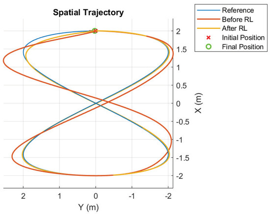
Figure 3.
Trajectory before and after RL; first case.
For a starting point at (2,0,3) that starts right at the beginning of the lemniscate curve, the controller, after learning a better set of gains, has a score (as defined in Equation (31)) of 0.0177, whereas the untuned controller produced a score of 0.1203. These results show a clear improvement in the trajectory tracking performance. The corresponding gain evolution in time is presented in Figure 4. The symbol t denotes discrete time. Hence, the scale is the number of samples, and continuous time elapsed since the beginning of the simulation is obtained by multiplying by the sampling period h.
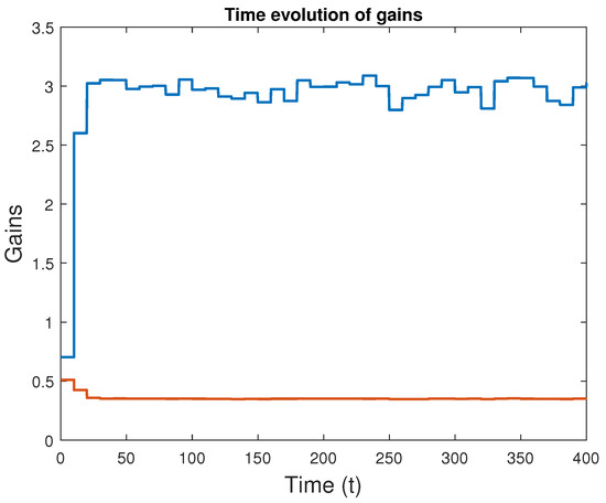
Figure 4.
Evolution of the learned attitude controller gains with time (first case: dither covariance ); the blue line represents the first gain and the red the second gain.
Despite some oscillations, the convergence is quick. This happens due to the selection of high variance for the dither noise. However, this procedure can be a problem, given that, in real life, quadrotors have limitations on the actuators that might render such high values impossible. The magnitudes of the input during the learning stage can induce big oscillations in the quadrotor, since the angular velocity and the angle get excited by the effect of the dither noise.
In order to be able to reduce the dither noise power and still obtain satisfactory results, an alternative is to increase the number of steps required for an update of the learned controller gains. However, this approach slows down the learning process. Another possibility is to increase the values of the covariance matrix of the LS estimator at each update so that the updates are less influenced by previous updates. This comes at the price of bigger oscillations. The new parameters are shown in Table 2.
Table 2.
Algorithm parameters for the second test.
With these updates, a new simulation rendered the results in Figure 5, which shows the evolution of the gains with time. Even though the learning process slows down as expected, improvements are still achieved. Figure 6 demonstrates that good trajectory tracking was obtained.
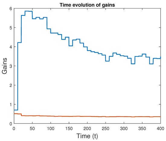
Figure 5.
Evolution of the learned attitude controller gains with time (second case: dither covariance ).
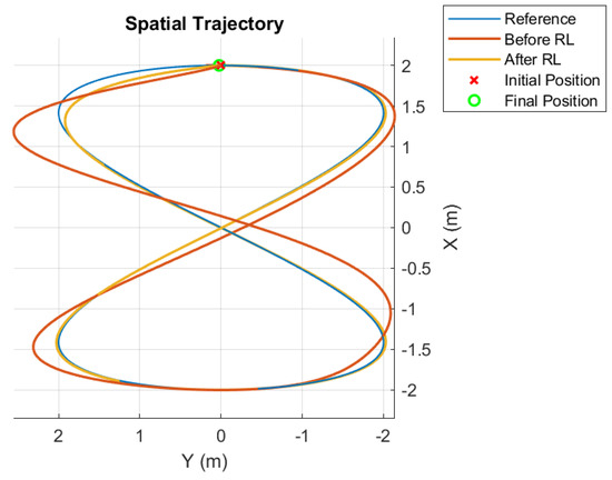
Figure 6.
Trajectory before and after RL; second case.
For a starting point at (2,0,3) that coincides with the beginning of the lemniscate curve, the controller performs reference tracking with a score (as defined in Equation (31)) of 0.0175 after the learning process, whereas the untuned controller produced a score of 0.1204, with the input torque acquiring smaller values as a direct consequence of the reduction in the dither noise.
5.2. Experiment 2
The previous two tests aim to improve the controller gains starting from non-optimum values. The following three tests try to improve on already optimized results.
The starting point for the controller gains corresponds to the following configuration of weights:
- Position controller: = diag(200,1), = 100;
- Attitude controller: = diag(100,1), = 10.
The difference between experiments is the value of the moment of inertia , which is assumed in each experiment to be:
- Third experiment Kg·m2;
- Fourth experiment Kg·m2;
- Fifth experiment Kg·m2.
The actual value of is 0.01 Kg·m2. This means that each experience has its attitude controller gains with values that are different from the optimal ones.
The algorithm has the same parameters throughout all three experiences, as presented in Table 3.
Table 3.
Algorithm parameters for the third, fourth, and fifth tests.
The dither is now significantly reduced, since less excitation is required.
The third experiment rendered the results shown in Figure 7 and Figure 8. A closer look at the trajectories reveals that improvements do occur, with the improved gains producing a better tracking performance. The score for the non-optimized version is 0.0202, whereas the version with learned gains scored 0.0175, reflecting a small improvement over the original configuration.
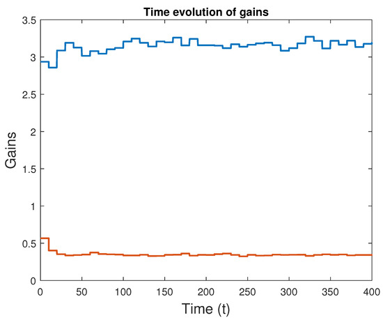
Figure 7.
Evolution of the learned attitude controller gains with time (third case: dither covariance ).
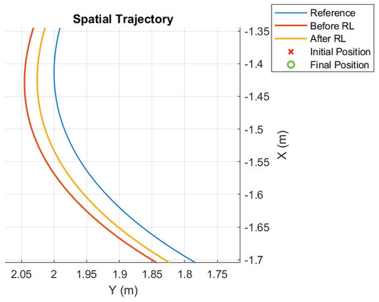
Figure 8.
Detail of the trajectory before and after RL; third case.
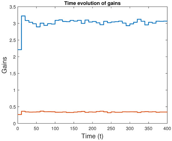
Figure 9.
Evolution of the learned attitude controller gains with time; fourth case.
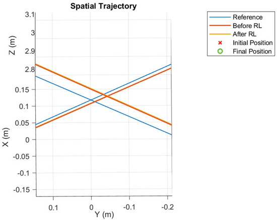
Figure 10.
Detail of the trajectory before and after RL; fourth case.
The score for the performance metric before the gains computed with RL are applied is 0.01781 and, after applying the algorithm, the score becomes 0.01765. In this case, the improvement is almost negligible. This can be seen in Figure 10, where both trajectories practically overlap each other, ending up having the same distance to the reference lemniscate curve.
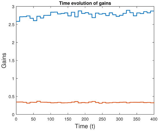
Figure 11.
Evolution of the learned attitude controller gains with time; fifth case.
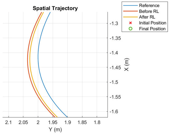
Figure 12.
Detail of the trajectory before and after RL; fifth case.
The score metric for the original set of gains is 0.01811 and, after applying the algorithm, the score becomes 0.01765. In this last experience, a small improvement was achieved. A good tuning of the algorithm allowed for a small performance improvement over a very optimized controller.
6. Conclusions
The development of a reinforcement learning-based adaptive controller for a quadrotor, which includes an adapted version of the Q-learning policy iteration algorithm for linear-quadratic problems, was performed. The particular class of RL-based controllers considered is such that it allows adaptation in real time.
Disturbances affecting the system input and output have a big effect on the correct functioning of the algorithm. A careful choice of algorithm parameters and balance between the estimation algorithm parameters is the solution to this problem. However, when big disturbances are present, it is only possible to make the gains converge close to optimality. Increasing the influence of prior estimations allows for a greater degree of robustness, with the drawback of deviating the convergence process to nearby values of the original optimal gains. Nonetheless, that is necessary to prevent harsh oscillations in the learned gains, which are still present in the quadrotor tests, most likely due to the non-linear nature of the rotational dynamics and other unmodeled dynamics besides the perturbations.
Still, the algorithm produced good results provided that the drone is kept working within the near-linear zone of operation, that is, where safe maneuvers with the quadrotor close to the hovering position are prevalent.
The selection of the dither noise power to inject must solve a dual problem. Indeed, the solution to the control problem requires a dither noise power as small as possible (ideally, zero), while the solution to the estimation problem requires a high value for the dither noise variance. The exact solution to this problem of finding the dither noise power value that fits the best compromise can be found by using multi-objective optimization, but it is computationally very heavy. Good approximations, such as the one proposed in [16], are available for predictive adaptive controllers. A possibility is then to try to adapt this approach to RL adaptive control, but a much more complicated algorithm is expected to arise. Although promising as future work, such a research track is outside the scope of the present work. Instead, in this article, the approach followed was to adjust the dither noise power by trial and error in order to obtain the best results.
Author Contributions
D.L.: research, implementation, writing; R.C.: research, methodology, writing; J.M.L.: research, methodology, writing. All authors have read and agreed to the published version of the manuscript.
Funding
Part of this work was supported by INESC-ID under project UIDB/50021/2020 and by LARSyS under project UIDB/50009/2020, both financed by Fundação para a Ciência e a Tecnologia (Portugal).
Institutional Review Board Statement
Not applicable.
Informed Consent Statement
Not applicable.
Data Availability Statement
The data are not publicly available. The data files are stored in corresponding instruments in personal computers.
Conflicts of Interest
The authors declare no conflicts of interest.
Abbreviations
The following abbreviations are used in this manuscript:
| RL | Reinforcement Learning |
| LQR | Linear Quadratic Regulator |
| VFA | Value Function Approximation |
| TD | Temporal Difference |
| RLS | Recursive Least-Squares |
| MDP | Markov Decision Process |
| ZOH | Zero-Order Hold |
References
- Kangunde, V.; Jamisola, R.S.; Theophilus, E.K. A review on drones controlled in real-time. Int. J. Dyn. Control 2021, 9, 1832–1846. [Google Scholar] [CrossRef] [PubMed]
- Azar, A.T.; Koubaa, A.; Ali Mohamed, N.; Ibrahim, H.A.; Ibrahim, Z.F.; Kazim, M.; Ammar, A.; Benjdira, B.; Khamis, A.M.; Hameed, I.A.; et al. Drone deep reinforcement learning: A review. Electronics 2021, 10, 999. [Google Scholar] [CrossRef]
- Elmokadem, T.; Savkin, A.V. Towards fully autonomous UAVs: A survey. Sensors 2021, 21, 6223. [Google Scholar] [CrossRef] [PubMed]
- Sutton, R.S.; Barto, A.G. Reinforcement Learning: An Introduction; MIT Press: Cambridge, MA, USA, 2018. [Google Scholar]
- Koch, W.; Mancuso, R.; West, R.; Bestavros, A. Reinforcement learning for UAV attitude control. ACM Trans.-Cyber-Phys. Syst. 2019, 3, 1–21. [Google Scholar] [CrossRef]
- Deshpande, A.M.; Minai, A.A.; Kumar, M. Robust deep reinforcement learning for quadcopter control. IFAC-PapersOnLine 2021, 54, 90–95. [Google Scholar] [CrossRef]
- Deshpande, A.M.; Kumar, R.; Minai, A.A.; Kumar, M. Developmental Reinforcement Learning of Control Policy of a Quadcopter UAV With Thrust Vectoring Rotors. In Proceedings of the Dynamic Systems and Control Conference, American Society of Mechanical Engineers, Pittsburgh, PA, USA, 4–7 October 2020; Volume 2, p. V002T36A011. [Google Scholar]
- Koh, S.; Zhou, B.; Fang, H.; Yang, P.; Yang, Z.; Yang, Q.; Guan, L.; Ji, Z. Real-time deep reinforcement learning based vehicle navigation. Appl. Soft Comput. 2020, 96, 106694. [Google Scholar] [CrossRef]
- Ramstedt, S.; Pal, C. Real-Time Reinforcement Learning. In Proceedings of the Advances in Neural Information Processing Systems, Vancouver, BC, Canada, 8–14 December 2019; Curran Associates, Inc.: Red Hook, NY, USA, 2019; Volume 32. [Google Scholar]
- Lillicrap, T.P.; Hunt, J.J.; Pritzel, A.; Heess, N.; Erez, T.; Tassa, Y.; Silver, D.; Wierstra, D. Continuous control with deep reinforcement learning. arXiv 2019, arXiv:1509.02971. [Google Scholar]
- Lewis, F.L.; Vrabie, D. Reinforcement learning and adaptive dynamic programming for feedback control. IEEE Circuits Syst. Mag. 2009, 9, 32–50. [Google Scholar] [CrossRef]
- Siciliano, B.; Sciavicco, L.; Villani, L.; Oriolo, G. Robotics; Advanced textbooks in control and signal processing; Springer: London, UK, 2009. [Google Scholar]
- Franklin, G.F.; Powell, J.D.; Workman, M.L. Digital Control of Dynamic Systems; Addison-Wesley: Reading, MA, USA, 1998; Volume 3. [Google Scholar]
- Recht, B. A tour of reinforcement learning: The view from continuous control. Annu. Rev. Control Robot. Auton. Syst. 2019, 2, 253–279. [Google Scholar] [CrossRef]
- Kulhavý, R. Restricted exponential forgetting in real-time identification. Automatica 1987, 23, 589–600. [Google Scholar] [CrossRef]
- da Silva, R.N.; Filatov, N.; Lemos, J.; Unbehauen, H. A dual approach to start-up of an adaptive predictive controller. IEEE Trans. Control. Syst. Technol. 2005, 13, 877–883. [Google Scholar] [CrossRef]
Disclaimer/Publisher’s Note: The statements, opinions and data contained in all publications are solely those of the individual author(s) and contributor(s) and not of MDPI and/or the editor(s). MDPI and/or the editor(s) disclaim responsibility for any injury to people or property resulting from any ideas, methods, instructions or products referred to in the content. |
© 2024 by the authors. Licensee MDPI, Basel, Switzerland. This article is an open access article distributed under the terms and conditions of the Creative Commons Attribution (CC BY) license (https://creativecommons.org/licenses/by/4.0/).