Analysis of Ultrasonic Wave Dispersion in Presence of Attenuation and Second-Gradient Contributions

Abstract

In this study, we aim to analyze the dispersion of ultrasonic waves due to second-gradient contributions and attenuation within the framework of continuum mechanics. To investigate dispersive behavior and attenuation effects, we consider the influence of both higher-order gradient terms (second gradients) and Rayleigh-type viscoelastic contributions. To this end, we employ the extended Rayleigh–Hamilton principle to derive the governing equations of the problem. Using a wave-form solution, we establish the relationship between the phase velocity and the material’s constitutive parameters, including those related to the stiffness of both standard (first-gradient) and second-gradient types, as well as viscosity. To validate the model, we use data available in the literature to identify all the material parameters. Based on this identification, we observe that our model provides a good approximation of the experimentally measured trends of both phase velocity and attenuation versus frequency. In conclusion, this result not only confirms that our model can accurately describe both wave dispersion and attenuation in a material, as observed experimentally, but also highlights the necessity of simultaneously considering both second-gradient and viscosity parameters for a proper mechanical characterization of materials.

1. Introduction

Ultrasonic wave propagation is a powerful technique used in a wide range of fields, from non-destructive testing (NDT) and material characterization to medical diagnostics. The study of how ultrasonic waves behave as they travel through materials provides essential information about the internal structure and mechanical properties of the materials being tested. In traditional models, wave propagation is typically described using classical elasticity theory, where the stress–strain relationship of the material depends on the first derivatives of the displacement field, representing the strain. Although this approach works well for simple, homogeneous materials, it is insufficient for more complex materials that possess microstructural heterogeneity or exhibit nonlocal interaction, since these materials often exhibit nonlocal behavior, meaning that the response at any given point in the material is influenced not only by the immediate surroundings but also by broader microstructural features. Second-gradient elasticity theory was developed to address this issue by introducing higher-order derivatives of the displacement field, which enables the model to capture these nonlocal effects and internal length scales within the material.

Since then, this theory has become particularly useful for modeling materials that exhibit scale-dependent behavior, such as foams, granular materials, and biological tissues. By incorporating second-gradient terms into the stress–strain relationship, this theory provides a more accurate description of wave propagation in materials with microstructural features, where the classical theory would not capture the complex interactions between the structure of the material and the propagating wave [1,2].

Dispersion refers to the phenomenon in which the speed of a wave depends on its frequency. In most classical wave propagation theories, the velocity of the wave is constant and independent of frequency. However, in second-gradient media, the wave velocity is frequency-dependent. This is because the material’s internal structure, captured, e.g., by the second-gradient terms, affects the wave’s propagation at different frequencies. This effect can be especially pronounced in materials where microstructural characteristics, such as pores, inclusions, or heterogeneity, influence wave propagation [3,4]. In practice, the dispersion observed in second-gradient media can lead to significant differences in how waves propagate, especially at higher frequencies. This has important implications for the design and analysis of materials such as metamaterials, where customizable dispersion characteristics are often desired to achieve specific effects, such as negative refraction or slow-wave propagation [5]. Similarly, in biological tissues, where wave dispersion is influenced by the cellular structure of the tissue, understanding dispersion becomes critical to improving medical imaging techniques such as ultrasound elastography [6].

Attenuation refers to the loss of energy that occurs when a wave propagates through a medium. In traditional wave theory, attenuation is typically associated with damping mechanisms, such as viscoelastic effects or material imperfections. However, in materials exhibiting second-gradient behavior, attenuation can arise due to the nonlocal interactions and microstructural features that influence wave propagation. As ultrasonic waves pass through a material with second-gradient effects, their energy is dissipated in a way that cannot be fully explained by classical damping models [7,8]. The attenuation in such materials is also frequency-dependent, with the energy loss being more significant at higher frequencies. This frequency-dependent attenuation is crucial for understanding wave behavior in biological tissues, where the microstructural properties of the tissue (such as cellular arrangements) can cause additional dissipation of wave energy. Similarly, in porous materials and composites, where waves interact with heterogeneities at multiple scales, the attenuation behavior provides valuable insight into the material’s internal structure and mechanical properties [9].

The theoretical framework of second-gradient elasticity, which includes both dispersion and attenuation effects, has several important applications. Understanding the frequency-dependent dispersion and attenuation can enhance the sensitivity and resolution of ultrasonic testing techniques, allowing for better detection of defects, cracks, or voids within materials [9]. In medical diagnostics, particularly in ultrasound elastography, these models can provide a more accurate representation of wave propagation through biological tissues. Since tissues often exhibit complex internal structures, the ability to account for nonlocal effects and microstructural interactions improves the precision of measurements, leading to more reliable assessments of tissue stiffness or elasticity. This has important implications for early diagnosis and monitoring of conditions such as tumors or liver fibrosis [6]. Additionally, the study of second-gradient effects in ultrasonic wave propagation is crucial for the development of metamaterials, engineered materials designed to have specific wave propagation characteristics. By tailoring the second-gradient parameters, researchers can design materials with bespoke dispersion and attenuation properties, opening up new possibilities for applications in sensing, communication, and imaging technologies [5]. Last but not least, we would like to highlight a recent contribution that has significantly inspired our work, specifically the thesis by Ronny Hofmann [10]. His study focuses on laboratory measurements of clastic rocks, ranging from 3 Hz to 500 kHz, and their application to well log analysis and a time-lapse study in the North Sea. Within this framework, the measurements reveal substantial dispersion in sandstones due to the saturation of inhomogeneities and open boundaries (such as pore pressure diffusion), which in turn affects the material’s compressibility and stiffness.

Furthermore, attenuation is directly related to the rate of change of the modulus. This concept is summarized in Figure 1 [10], which illustrates that as the parameter $\mu$ (defined in Hofmann’s thesis [10] as a distribution parameter that gives the range over which a relaxation mechanism operates) changes, i.e., from 0.8 to 0.2, the dispersion of phase velocities is higher as in Figure 1a, and the attenuation peaks in Figure 1b become more pronounced. Figure 1c summarizes the content presented in Figure 1a,b, which are taken from Hofmann’s thesis, and then illustrates how the phase velocity varies as a function of frequency $\omega$ and how this variation is closely associated with attenuation behavior, both influenced by the parameter $\mu$. The blue curve represents the frequency-dependent phase velocity $v_{p1}$, which exhibits dispersion—meaning that the phase velocity increases with frequency. This increase is particularly evident around the frequency where attenuation reaches its maximum. The black curve shows the attenuation trend, which peaks at a specific frequency marked by the vertical dashed magenta line. At this point, the energy loss within the material is at its highest due to internal viscosity. The green line indicates the reference phase velocity $v_l$ at low frequencies, representing the asymptotic limit as frequency approaches zero. Conversely, the red line corresponds to the high-frequency limit $v_h$, where dispersion effects diminish and the phase velocity stabilizes. Overall, the figure highlights that the most significant change in phase velocity occurs near the frequency where attenuation peaks.

Since no continuous model currently exists that can capture the aforementioned effect, the aim of this research is to provide a model that, starting from the Rayleigh–Hamilton principle and considering both the material’s internal viscosity and second-gradient parameters, can simulate the aforementioned dispersive and dissipative effects.

Besides the Introduction, the paper is organized into the following sections:

• Section 2 outlines the construction of the governing equations based on the Hamilton–Rayleigh principle, considering both internal viscosity and second-gradient parameters of the material. Starting from the dispersion equation and using the wave-form solution, we derive the wave number and then the phase velocity and the quality factor for the evaluation of attenuation phenomena. Once the methodology and model have been finalized, we search for materials and experimental data from the literature to validate the model.
• Section 3 focuses on the validation of the above model. Three case studies from the literature (one involving natural materials and two involving artificial materials) are examined. The purpose is to compare experimental data with the numerical simulation results derived from the model. Results and comments on the above-mentioned comparison are also discussed in this section. Moreover, we have introduced a numerical simulation to evaluate general aspects of the wave’s behavior, from the perspectives of both dispersion and attenuation.
• Finally, Section 4 offers our conclusions and reflections on future developments, and it reports all the contributions.

A list of abbreviations used in the manuscript and all the references adopted for this study are presented at the end of the article. Furthermore, at the end of the publication, we have added an Appendix A to revisit and further elaborate on topics addressed during the modeling phase.

2. Modeling and Methods

2.1. Scope and Strategy

We are searching for a model that can reproduce the variation of phase velocity and attenuation with wave frequency for a given material, as shown in Figure 1c, which is our benchmark. In this context, we will consider the Rayleigh–Hamilton principle, using second-gradient and viscous parameters to describe the displacement involved in the energies represented in the principle. The Partial Differential Equation (PDE) obtained will be solved using a wave-form solution to derive the dispersion equation that includes phase velocity and attenuation.

2.2. Variational Derivation of Governing Equations (PDE and BCs)

We begin by recalling the extended Rayleigh–Hamilton principle, which postulates that the variation of the Action, $\delta A$, is connected to the Rayleigh function R:

$$\delta A={\int }_{t_0}^{t_1}\left\{{\int }_0^L\left(\delta K-\delta W^{\mathrm{int}}\right)dx+\delta W^{\mathrm{ext}}\right\}dt={\int }_{t_0}^{t_1}\left({\displaystyle \frac{\delta R}{\delta {\dot{u}}^{\prime }}}\delta u^{\prime }+{\displaystyle \frac{\delta R}{\delta {\dot{u}}^{″}}}\delta u^{″}\right)dt,$$

(1)

where the three energy functions K, the kinetic energy density, W, the potential energy density, $W^{\mathrm{int}}$, the internal energy per unit volume, and $W^{\mathrm{ext}}$, the external energy function, are defined as

$$K={\int }_0^L\left({\displaystyle \frac{1}{2}}\rho {\dot{u}}^2+{\displaystyle \frac{1}{2}}\eta {\dot{u^{\prime }}}^2\right)dx,$$

(2)

$$W^{\mathrm{int}}={\int }_0^L\left({\displaystyle \frac{1}{2}}{k}_1{u}^{\prime 2}+{\displaystyle \frac{1}{2}}{k}_2{u}^{″2}\right)dx,$$

(3)

$$W^{\mathrm{ext}}={\left[F_0^{\mathrm{ext}}u+B_0^{\mathrm{ext}}{u}^{\prime }\right]}_{x=0}+{\left[F_L^{\mathrm{ext}}u+B_L^{\mathrm{ext}}{u}^{\prime }\right]}_{x=L}+{\int }_0^L(b_{n}u+b_d{u}^{\prime })dx,$$

(4)

and the Rayleigh function is equal to

$$R={\int }_0^L\left({\displaystyle \frac{1}{2}}{c}_1{\dot{u}}^{\prime 2}+{\displaystyle \frac{1}{2}}{c}_2{\dot{u}}^{″2}\right)dx$$

(5)

We recall that $k_1$ and $k_2$ are the standard elastic modulus for a linear one-dimensional elastic body and the non-standard strain-gradient modulus, respectively. Given the displacement u, its derivatives with respect to time are denoted by $\dot{u}$, with respect to space by $u^{\prime }$ (first derivative) or $u^{″}$ (second derivative). $\rho$ and $\eta$ are the mass density (mass per unit length) and the micro-inertia of the one-dimensional body, respectively. $b_n$ and $b_d$ are the external distributed (per unit length) forces and double forces, respectively. $F_0^{\mathrm{ext}}$ (or $F_L^{\mathrm{ext}}$) and $B_0^{\mathrm{ext}}$ (or $B_L^{\mathrm{ext}}$) are the concentrated forces and double forces evaluated at the extrema $x=0$ (or $x=L$) of the one-dimensional body, respectively.

Meanwhile, in the Rayleigh function, two internal viscosities are present: $c_1$, related to the first gradient field, and $c_2$, related to the second-gradient field.

Replacing (2), (3), (4), and (5) in the left side of Equation (1) and integrating by parts, for every admissible variation of the displacement field, the variation of the Action, $\delta A$, can be reduced to

$$\begin{array}{cc}\hfill \delta A=& {\int }_{t_0}^{t_1}\left\{{\int }_0^L\left[\delta u\left(-\rho \ddot{u}+k_1{u}^{″}+\eta {\ddot{u}}^{″}-k_2{u}^{\left(4\right)}+b_n-b_d^{\prime }\right)\right]dx\right\}\hfill \\ & -{\int }_{t_0}^{t_1}\delta u(x=0)\left[-\eta {\ddot{u}}^{\prime }(x=0)-k_1{u}^{\prime }(x=0)+k_2{u}^{″\prime }(x=0)+b_d\right]dt\hfill \\ & +{\int }_{t_0}^{t_1}\delta u(x=L)\left[-\eta {\ddot{u}}^{\prime }(x=L)-k_1{u}^{\prime }(x=L)+k_2{u}^{″\prime }(x=L)+b_d\right]dt\hfill \\ & -{\int }_{t_0}^{t_1}\delta u^{\prime }(x=0)\left[-k_2{u}^{″}(x=0)\right]dt\hfill \\ & +{\int }_{t_0}^{t_1}\delta u^{\prime }(x=L)\left[-k_2{u}^{″}(x=L)\right]dt.\hfill \end{array}$$

(6)

The variation of the Rayleigh function is

$${\int }_{t_0}^{t_1}\left({\displaystyle \frac{\delta R}{\delta {\dot{u}}^{\prime }}}\delta u^{\prime }+{\displaystyle \frac{\delta R}{\delta {\dot{u}}^{″}}}\delta u^{″}\right)dt={\int }_0^t{\int }_0^L\left(c_1{\dot{u}}^{\prime }\delta u^{\prime }+c_2{\dot{u}}^{″}\delta u^{″}\right)dxdt,$$

(7)

which, after integrating by parts in space and time, becomes

$$\begin{array}{cc}\hfill {\int }_{t_0}^{t_1}\left({\displaystyle \frac{\delta R}{\delta {\dot{u}}^{\prime }}}\delta u^{\prime }+{\displaystyle \frac{\delta R}{\delta {\dot{u}}^{″}}}\delta u^{″}\right)dt=& {\int }_{t_0}^{t_1}{\left[c_1{\dot{u}}^{\prime }\delta u\right]}_0^{L}dt-{\int }_{t_0}^{t_1}{\int }_0^L{c}_1{\dot{u}}^{″}\delta udxdt\hfill \\ & +{\int }_{t_0}^{t_1}{\left[c_2{\dot{u}}^{″}\delta u^{\prime }\right]}_0^{L}dt-{\int }_{t_0}^{t_1}{\left[c_2{\dot{u}}^{″\prime }\delta u\right]}_0^{L}dt\hfill \\ & +{\int }_{t_0}^{t_1}{\int }_0^L{c}_2{\dot{u}}^{\left(4\right)}\delta udxdt.\hfill \end{array}$$

(8)

Then, inserting Equations (8) and (6) into (1) and rearranging, we obtain

$$\begin{array}{cc}\hfill \delta A=& {\int }_{t_0}^{t_1}\left\{{\int }_0^L\left[\delta u\left(-\rho \ddot{u}+k_1{u}^{″}+\eta {\ddot{u}}^{″}-k_2{u}^{\left(4\right)}+b_n-b_d^{\prime }+c_1{\dot{u}}^{″}-c_2{\dot{u}}^{\left(4\right)}\right)\right]dx\right\}dt\hfill \\ & -{\int }_{t_0}^{t_1}\delta u(x=0)\left[-\eta {\ddot{u}}^{\prime }(x=0)-k_1{u}^{\prime }(x=0)+k_2{u}^{″\prime }(x=0)+b_d\right.\hfill \\ & \left.-c_1{\dot{u}}^{\prime }(x=0)+c_2{\dot{u}}^{″\prime }(x=0)\right]dt\hfill \\ & +{\int }_{t_0}^{t_1}\delta u(x=L)\left[-\eta {\ddot{u}}^{\prime }(x=L)-k_1{u}^{\prime }(x=L)+k_2{u}^{″\prime }(x=L)+b_d\right.\hfill \\ & \left.-c_1{\dot{u}}^{\prime }(x=L)+c_2{\dot{u}}^{″\prime }(x=L)\right]dt\hfill \\ & -{\int }_{t_0}^{t_1}\delta u^{\prime }(x=0)\left[-k_2{u}^{″}(x=0)-c_2{\dot{u}}^{″}(x=0)\right]dt\hfill \\ & +{\int }_{t_0}^{t_1}\delta u^{\prime }(x=L)\left[-k_2{u}^{″}(x=L)-c_2{\dot{u}}^{″}(x=L)\right]dt=0.\hfill \end{array}$$

(9)

where, since the displacement $u(x,t)$ is assumed to be prescribed both at $t=t_0$ and at $t=t_1$, we have that $\delta u(x,t=t_0)=\delta u(x,t=t_1)=0$. Equation (9) must hold for every admissible variation $\delta u$ of the displacement field u. Therefore, the last four terms of Equation (9) must be null. On one hand, if the displacement u or the displacement gradient $u^{\prime }$ are prescribed at the boundary (i.e., the left-hand sides of the following equations are satisfied), then their variation is null, as well as the corresponding terms in Equation (9). On the other hand, if these kinematic conditions are not prescribed, then the right-hand sides of the following equations must be satisfied to make the same terms of Equation (9) null:

$$\begin{array}{cc}\hfill u(0,t)& =u_0\left(t\right)\hfill \\ \hfill \mathrm{or}& -\eta {\ddot{u}}^{\prime }(x=0,t)-k_1{u}^{\prime }(x=0,t)+k_2{u}^{″\prime }(x=0,t)+b_d\hfill \\ \hfill & -c_1{\dot{u}}^{\prime }(x=0,t)+c_2{\dot{u}}^{″\prime }(x=0,t)=F_0^{\mathrm{ext}},\hfill \end{array}$$

(10)

$$\begin{array}{cc}\hfill u(L,t)& =u_L\left(t\right)\hfill \\ \hfill \mathrm{or}& -\eta {\ddot{u}}^{\prime }(x=L,t)-k_1{u}^{\prime }(x=L,t)+k_2{u}^{″\prime }(x=L,t)+b_d\hfill \\ \hfill & -c_1{\dot{u}}^{\prime }(x=L,t)+c_2{\dot{u}}^{″\prime }(x=L,t)=-F_L^{\mathrm{ext}},\hfill \end{array}$$

(11)

$$\begin{array}{c}\hfill \begin{array}{ccccc}\hfill u^{\prime }(0,t)& =b_0\left(t\right)\hfill & \hfill \mathrm{or}& -k_2{u}^{″}(x=0,t)-c_2{\dot{u}}^{″}(x=0,t)\hfill & \hfill =B_0^{\mathrm{ext}}\left(t\right),\end{array}\end{array}$$

(12)

$$\begin{array}{c}\hfill \begin{array}{ccccc}\hfill u^{\prime }(L,t)& =b_L\left(t\right)\hfill & \hfill \mathrm{or}& -k_2{u}^{″}(x=L,t)-c_2{\dot{u}}^{″}(x=L,t)\hfill & \hfill =-B_L^{\mathrm{ext}}\left(t\right).\end{array}\end{array}$$

(13)

for every instant of time, e.g., $\forall t\in \mathbb{R}$. Finally, the first line of Equation (9) must also be zero for every admissible variation $\delta u$ of the displacement field. Thus, because of its arbitrariness, it follows that

$$-\rho \ddot{u}+k_1{u}^{″}+\eta {\ddot{u}}^{″}-k_2{u}^{\left(4\right)}-b_d^{\prime }+b_n+c_1{\dot{u}}^{″}-c_2{\dot{u}}^{\left(4\right)}=0,\forall x\in [0,L],\forall t\in \mathbb{R}.$$

(14)

2.3. Wave-Form Solution

Equation (14) is the Partial Differential Equation (PDE) governing the evolution of the displacement field $u(x,t)$ for the investigated model, which will be solved in the following two subsections. In particular, we look for a wave-form solution to (14), and we assume the body length L to be sufficiently large so that the boundary conditions (BCs) (10)–(13) do not influence the solution.

Equation (14) can be solved by considering no external distributed actions ($b_n=0$ and $b_d=0$), in the form of the following plane wave solution for the displacement field:

$$u(x,t)=\mathrm{Re}\left(u_0{e}^{i(\omega t-k_{\omega }x)}\right),$$

(15)

where $u_0$ is the complex wave amplitude, $\omega$ is the frequency of the wave expressed in rad/s, $k_{\omega }$ is the complex wave number, i is the imaginary unit, and Re is the real part operator. Calculating the derivatives of (15) and inserting them into (14), it results in

$$(k_2+i{c}_2\omega )k_{\omega }^4+(k_1+i{c}_1\omega -\eta {\omega }^2)k_{\omega }^2-\rho {\omega }^2=0,$$

(16)

where the arbitrariness of the complex wave amplitude $u_0$ has been considered. Equation (16) is a fourth-degree algebraic equation in terms of $k_{\omega }$ and therefore admits four complex solutions for $k_{\omega }$. However, in (16), $k_{\omega }$ appears only with even powers ($k_{\omega }^2$ or $k_{\omega }^4$). Thus, if $k_{\omega }={\widehat{k}}_{\omega }$ is a solution of (16), then $k_{\omega }=-{\widehat{k}}_{\omega }$ is also a solution. As a consequence, two of these solutions correspond to right-hand propagating waves, while the other two are equal in magnitude and opposite in sign. The reason is the isotropy of the domain. In the formulae, two independent solutions are

$$k_{{\omega }_{1,2}}=\sqrt{{\displaystyle \frac{-(k_1+i{c}_1\omega -\eta {\omega }^2)\pm \sqrt{{(k_1+i{c}_1\omega -\eta {\omega }^2)}^2+4(k_2+i{c}_2\omega )\left(\rho {\omega }^2\right)}}{2(k_2+i{c}_2\omega )}}}.$$

(17)

Remembering the correlation between frequency $\omega$, wave number $k_{\omega }$, and phase velocity $v_p$ [11], we obtain an expression for the two phase velocities:

$$\begin{array}{cc}\hfill v_{p_{1,2}}& =\mathrm{Re}\left({\displaystyle \frac{\omega }{k_{{\omega }_{1,2}}}}\right)=\hfill \\ \hfill & =\mathrm{Re}\left(\sqrt{{\displaystyle \frac{2(k_2+i{c}_2\omega ){\omega }^2}{-(k_1+i{c}_1\omega -\eta {\omega }^2)\pm \sqrt{{(k_1+i{c}_1\omega -\eta {\omega }^2)}^2+4(k_2+i{c}_2\omega )\left(\rho {\omega }^2\right)}}}}\right).\hfill \end{array}$$

(18)

Similarly, starting from the wave number $k_{\omega }$, it is possible to determine the two corresponding quality factors $Q_1$ and $Q_2$ [10] as the inverse of the damping ratio $\zeta$, which characterizes the rate of energy loss in the system, expressed as a function of the real and imaginary parts of the wave number:

$$\begin{array}{c}\hfill {\zeta }_{1,2}={\displaystyle \frac{1}{Q_{1,2}}}=-{\displaystyle \frac{Im\left(k_{{\omega }_{1,2}}\right)}{Re\left(k_{{\omega }_{1,2}}\right)}}.\end{array}$$

(19)

The quality factors can also be understood as the ratio between stored and dissipated energy [10]. The quality factor has two definitions in the literature, which yield approximately the same value when $Q\gg 1$, as is the case for seismic waves. These definitions are given in terms of twice the strain energy and the total energy, respectively, both time-averaged over a cycle [12]. In conclusion, Equations (18) and (19) serve as the reference for our model, linking phase velocity and attenuation to the frequency of the wave propagating through the material. Figure 2 presents the results of our theoretical model, based on the constitutive framework and equations introduced in this manuscript (notably Equations (18) and (19)). In summary, Figure 1 is qualitative and illustrative, derived from Hofmann’s experimental work, whereas Figure 2 is quantitative, based on our theoretical development, and directly supports the validation of the proposed model.

3. Validation: Results and Discussion

3.1. Introduction

As already highlighted in the Introduction of this manuscript, we want to validate this model with data available for common construction materials in the literature [13,14]. Such literature has been selected because, among many available articles, both phase velocity and attenuation measurements have been made for the same material at the same frequencies.

In detail, we investigate a sandstone sample [13], a cement paste sample [14], and finally a concrete sample [14]. For each material, we have developed a case study; then, the validation is obtained by superimposing the theoretical predictions (obtained from numerical simulations) with the experimental data.

First, we propose a numerical simulation that allows us to make general considerations about the dispersive behavior of the wave, characteristic of our model. Second, we validate the model using the materials presented above, comparing the available experimental data with the numerical simulation. The material constitutive parameters used in this section are presented in

Table 1. Table of constitutive parameters for different figures.

Reference	Figure nr.	Constitutive Parameters
		${\mathit{k}}_{\mathbf{1}}$	${\mathit{k}}_{\mathbf{2}}$	$\mathit{\rho }$	$\mathit{\eta }$	${\mathit{c}}_{\mathbf{1}}$	${\mathit{c}}_{\mathbf{2}}$
		$\left[\mathbf{kg}{\mathbf{m}}^{\mathbf{-}\mathbf{1}}{\mathbf{s}}^{\mathbf{-}\mathbf{2}}\right]$	$\left[\mathbf{kg}\mathbf{m}{\mathbf{s}}^{\mathbf{-}\mathbf{2}}\right]$	$\left[\mathbf{kg}{\mathbf{m}}^{\mathbf{-}\mathbf{3}}\right]$	$\left[\mathbf{kg}{\mathbf{m}}^{\mathbf{-}\mathbf{1}}\right]$	$\left[\mathbf{kg}{\mathbf{m}}^{\mathbf{-}\mathbf{1}}{\mathbf{s}}^{\mathbf{-}\mathbf{1}}\right]$	$\left[\mathbf{kg}\mathbf{m}{\mathbf{s}}^{\mathbf{-}\mathbf{1}}\right]$
benchmark 1	2	1	0.5	1	0.1	1	1 × ${10}^{-3}$
benchmark 2	3	1	0.5	1	0.1	3	1 × ${10}^{-3}$
sandstone	4	7.7 × ${10}^9$	0.1 × ${10}^6$	2650	0.04	100	5 × ${10}^{-3}$
cement paste	5	11.3 × ${10}^9$	1.8 × ${10}^6$	1500	0.253	23.8 × ${10}^3$	1 × ${10}^{-3}$
concrete	6	37.3 × ${10}^9$	33.5 × ${10}^6$	2450	1.4	300 × ${10}^3$	1 × ${10}^{-3}$

.

Figure 2 and Figure 3 refer to the numerical simulation toward the benchmark (Figure 1), while Figure 4, Figure 5 and Figure 6 refer to the case studies.

3.2. Numerical Simulation Toward the Benchmark

Figure 2 presents a graphical representation of the two phase velocities (18) and their respective attenuations (19) computed using the material parameters listed in Table 1. When $c_1$ and $c_2$ are set to zero, $v_{p2}$ becomes zero, while $v_{p1}$ asymptotically approaches the low-frequency velocity $v_l$ and the high-frequency velocity $v_h$, defined as follows:

$$\underset{\omega \to 0}{lim}\underset{c_1\to 0}{lim}\underset{c_2\to 0}{lim}{v}_{p_{1,2}}=v_l=\sqrt{{\displaystyle \frac{k_1}{\rho }}},$$

(20)

$$\underset{\omega \to \infty }{lim}\underset{c_1\to 0}{lim}\underset{c_2\to 0}{lim}{v}_{p_{1,2}}=v_h=\sqrt{{\displaystyle \frac{k_2}{\eta }}},$$

(21)

For $c_1$ and $c_2$ different from zero, Figure 2 shows that the wave with phase velocity $v_{p2}$ exhibits significantly higher attenuation than the wave with phase velocity $v_{p1}$, rendering it experimentally unmeasurable. Moreover, the transition of velocity from low- to high-frequency regimes occurs at a characteristic frequency for both waves, corresponding to the attenuation peak. For certain values of the viscosities $c_1$ and $c_2$, as illustrated in Figure 3, a jump in the phase velocities $v_{p_1}$ and $v_{p_2}$ is observed at the frequency where the attenuation curves of both signals share a common peak. Nevertheless, the phase velocity measurable by ultrasonic instruments will always correspond to the wave with lower attenuation, namely $v_{p_1}$ in the numerical example considered.

3.3. Validation with Data from Literature

Since experimental attenuation measurements available in the literature are generally expressed as the loss of signal amplitude between one end and the other of the sample along its length L and are measured in (dB/m), it is useful to introduce an attenuation coefficient $\alpha$, according to the following formulation [13]:

$$\alpha =-{\displaystyle \frac{20}{x}}·log\left({\displaystyle \frac{u_x}{u_0}}\right),$$

(22)

where $u_0$ and $u_x$ denote the complex wave amplitudes at the source location and at a generic position x, respectively, along the propagation direction through the medium. Inserting (15) into (22), using the Euler properties and considering the real and imaginary parts of the wave number, we obtain

$$\alpha =-20i{k}_{\omega }\approx 20\mathrm{Im}\left(k_{\omega }\right),$$

(23)

where in the wave number we can omit the real part since, due to the fact that we use maximum values of amplitude in (23), the cosine of the wave number, corresponding to its real part, assumes values that are certainly lower than those related to the imaginary part. Once the material stiffness parameters, microstructure, micro-inertias, and density are set, the next step is to evaluate how variations in the internal viscosity of the material influence the combination of parameters that best approximate the experimental data for phase velocity and attenuation.

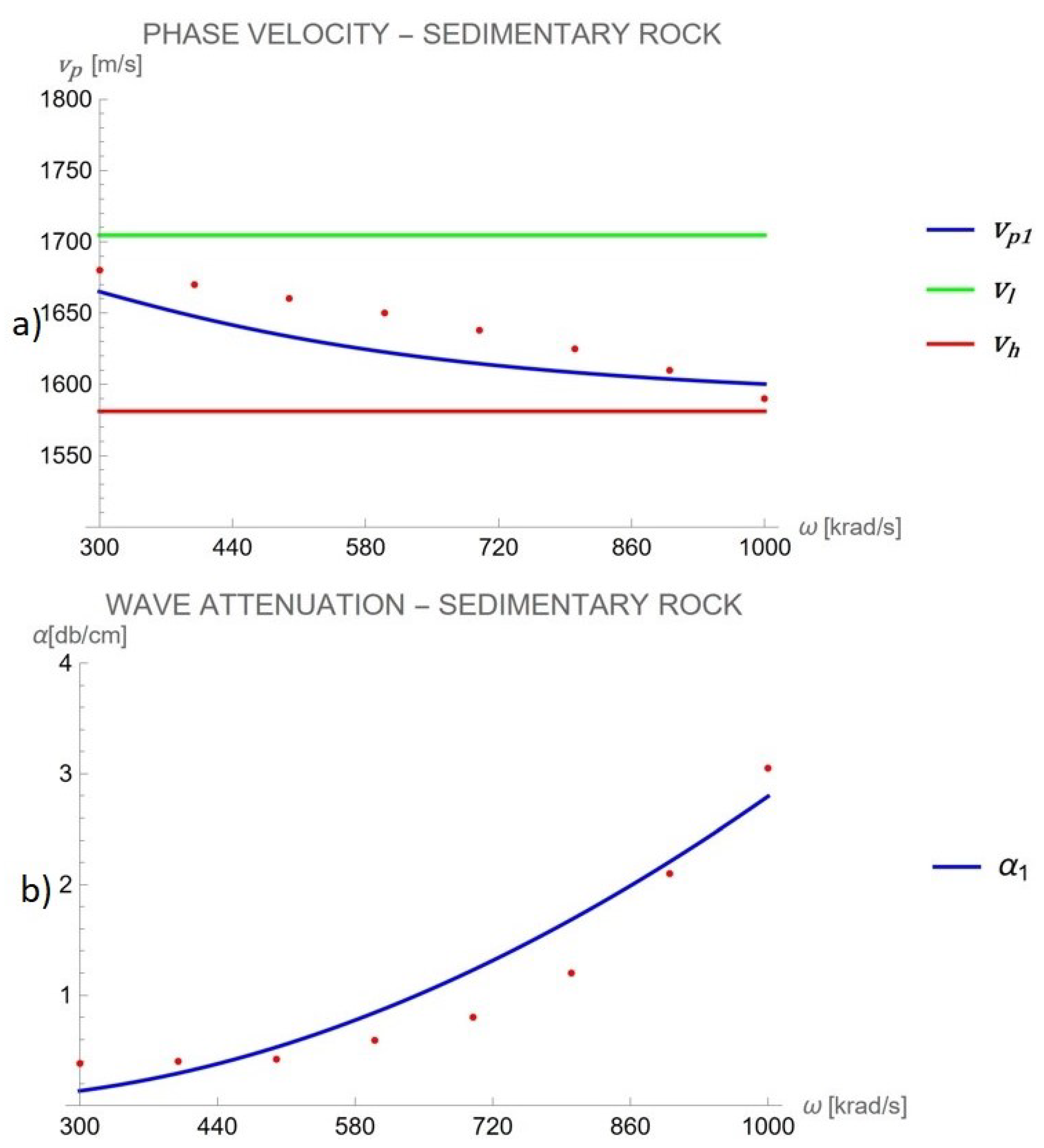
3.3.1. First Case of Study: Sandstone

The sediment specimen was prepared in a 100 mm × 100 mm × 50 mm container immersed in water to optimize velocity dispersion and minimize ultrasonic pulse attenuation [13]. The experiment took place in a 650 mm × 750 mm × 1500 mm water bath, using two matched pairs of broadband transducers with center frequencies of 0.5 MHz and 1.0 MHz [13]. The transducers were aligned coaxially with a 150 mm separation, mounted on a stable frame to ensure accurate wave amplitude measurements and prevent pressure variations on the probes [13].

In this case study, we already know the bulk modulus of the material and its density, so the phase velocity for the low-frequency regime is immediately obtained by Equation (20). The values of microstructure and micro-inertia can be derived by calculating the characteristic length of the material, taking into account that the velocity in the high-frequency regime is lower than that in the low-frequency regime according to experimental data.

In Figure 4, we present the overlap between numerical simulation, using the constitutive parameters of Table 1, and experimental data for phase velocity and wave attenuation in the tested material. In the frequency range of investigation, no attenuation peak is observed. The monotonic trend observed in both phase velocity (decreasing) and attenuation (increasing) is successfully captured by the numerical simulation, confirming the model’s accuracy in describing wave propagation behavior.

Table 2. Ultrasonic wave velocities and attenuation for sandstone sample: comparison between theoretical (Theo.) and experimental (Exp.) values.

$\mathit{\omega }$ (kHz)	Theo. ${\mathit{v}}_{\mathit{p}}$ (m/s)	Exp. ${\mathit{v}}_{\mathit{p}}$ (m/s)	Theo. $\mathit{\alpha }$	Exp. $\mathit{\alpha }$
300	1665.03	1680	0.1338	0.38
400	1647.69	1670	0.2928	0.40
500	1633.53	1660	0.5291	0.42
600	1622.66	1650	0.8417	0.59
700	1614.49	1638	1.2273	0.80
800	1608.36	1625	1.6828	1.20
900	1603.73	1610	2.2061	2.10
1000	1600.18	1590	2.7954	3.05

summarizes the theoretical and experimental ultrasonic wave velocities measured in the sandstone sample at frequencies ranging from 300 kHz to 1000 kHz. To evaluate the accuracy of the theoretical model, the Root Mean Square Error (RMSE) between the theoretical and experimental velocities was calculated. The RMSE value of approximately 19.82 m/s corresponds to 1.21% relative to the average theoretical velocity, indicating very good agreement between theoretical predictions and experimental results.

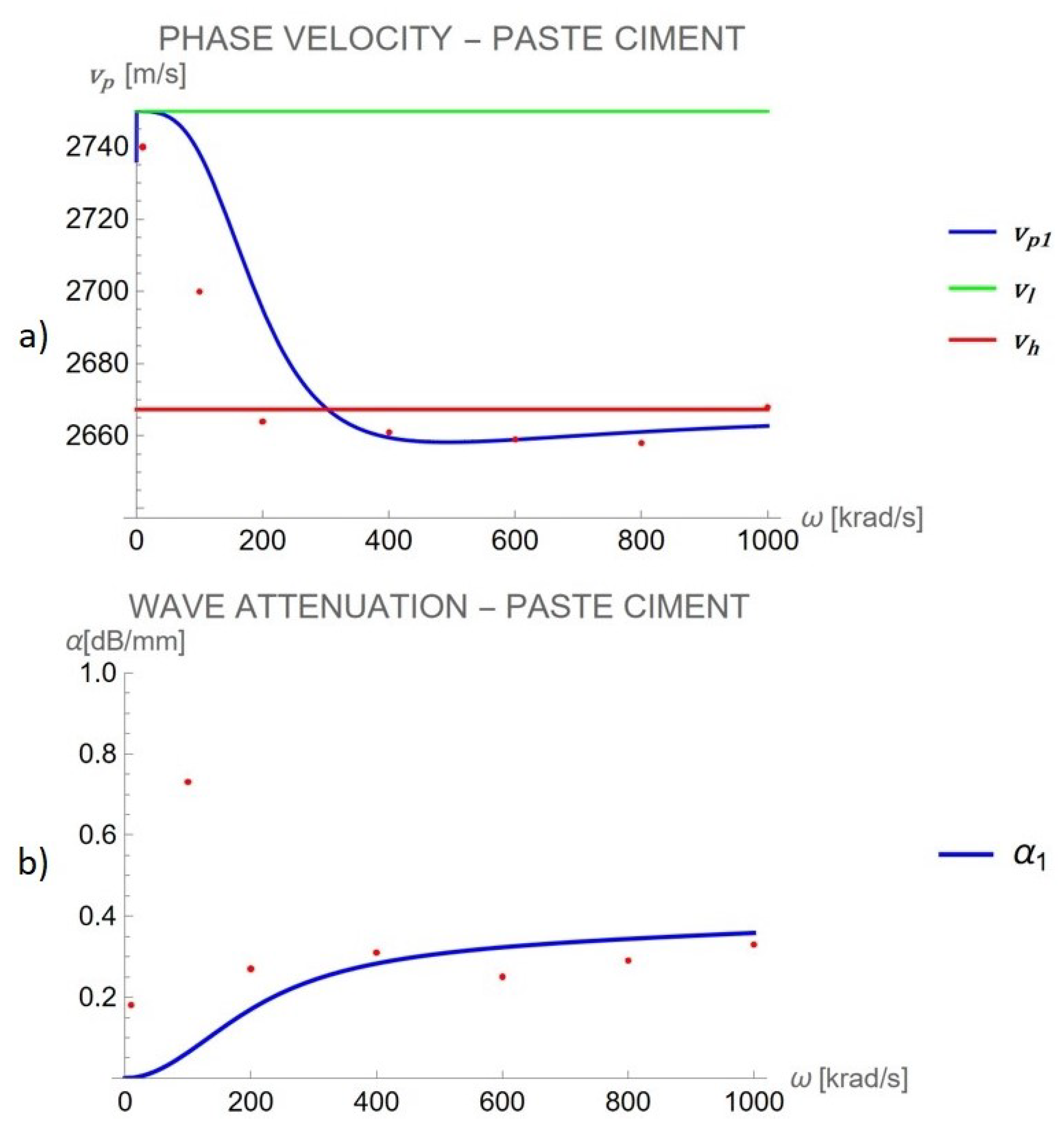
3.3.2. Second Case of Study: Cement Paste

The specimens tested were cubic with 150 mm edges. The experimental setup uses a simple through-transmission ultrasonic configuration, employing a wave-form generator board and two broadband transducers with frequencies between 100 kHz and 1 MHz, along with a data acquisition system [14]. We consider the data for a sample with water/cement ratio = 0.375 [14].

In Figure 5, we compare experimental data with the numerical simulation of the model. The phase velocity suddenly decreases around 200 kHz, tending towards the high-frequency regime velocity. In the attenuation plot, an increasing trend is observed, although a resonance peak appears at 100 kHz in the experimental data, probably due to effects not captured by the model such as internal micro-fractures with fluid inclusions or measurement errors.

Table 3. Ultrasonic wave velocities and attenuation for cement paste (w/c = 0.375): comparison between theoretical (Theo.) and experimental (Exp.) values.

$\mathit{\omega }$ (kHz)	Theo. ${\mathit{v}}_{\mathit{p}}$ (m/s)	Exp. ${\mathit{v}}_{\mathit{p}}$ (m/s)	Theo. $\mathit{\alpha }$	Exp. $\mathit{\alpha }$
10	2749.97	2740	0.00076	0.18
100	2738.17	2700	0.06341	0.73
200	2694.98	2664	0.17002	0.27
400	2659.52	2661	0.28302	0.31
600	2658.95	2659	0.32307	0.25
800	2661.11	2658	0.34370	0.29
1000	2662.75	2668	0.35856	0.33

summarizes the theoretical and experimental ultrasonic wave velocities measured in the cement paste sample for frequencies ranging from 10 kHz to 1000 kHz. As also observed in the sandstone case, discrepancies between experimental and theoretical results increase slightly at higher frequencies. These discrepancies may arise from frequency-dependent attenuation mechanisms and effects of second-gradient parameters (e.g., micro-inertia), which become significant at high frequencies when the wavelength approaches the size of the microstructure. To evaluate the accuracy of the theoretical model, the Root Mean Square Error (RMSE) between the theoretical and experimental velocities was calculated. The RMSE value of approximately 19.10 m/s corresponds to 0.71% relative to the average theoretical velocity, indicating very good agreement between theoretical predictions and experimental results.

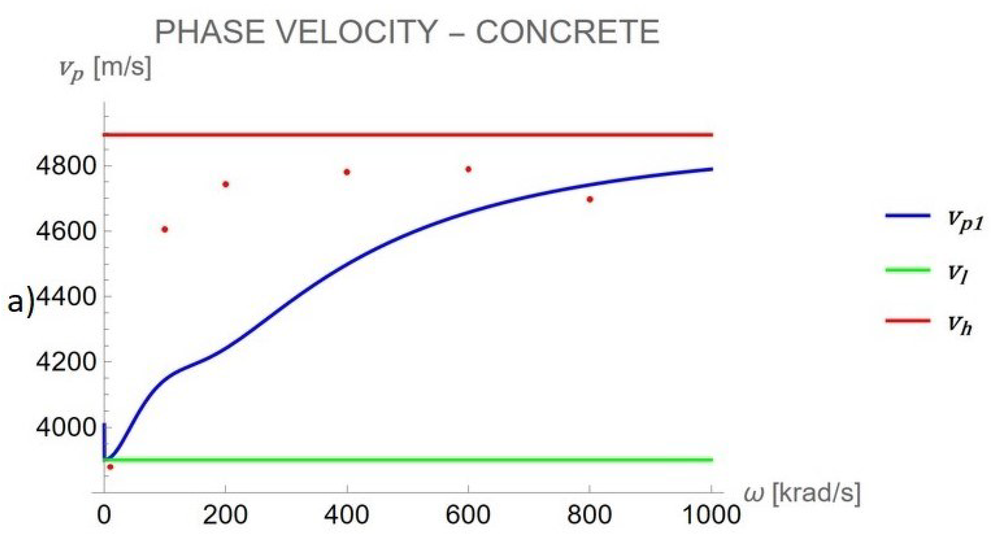
3.3.3. Third Case of Study: Concrete

As for the cement paste, the specimens tested were cubic of 150 mm edge, and the experimental setup was the same as the previous case of study [14]. Several different compositions of concrete were manufactured in the functions of water to cement ratio and of aggregate to cement ratio for a total of 24 specimens [14]. We consider the data for a sample with water/cement ratio = 0.375 [14]. Also, in this case the model confirms the monotonic trend of the experimental data [14] (see Figure 6).

Table 4. Ultrasonic wave velocities and attenuation for concrete sample (a/c = 3, w/c = 0.375): comparison between theoretical (Theo.) and experimental (Exp.) values.

$\mathit{\omega }$ (kHz)	Theo. ${\mathit{v}}_{\mathit{p}}$ (m/s)	Exp. ${\mathit{v}}_{\mathit{p}}$ (m/s)	Theo. $\mathit{\alpha }$	Exp. $\mathit{\alpha }$
10	3907.19	3879	0.002038	0.03
100	4145.15	4605	0.114637	0.17
200	4240.98	4743	0.242419	0.19
400	4498.14	4780	0.348456	0.33
600	4656.95	4789	0.387680	0.38
800	4741.50	4697	0.406327	0.42

summarizes the theoretical and experimental ultrasonic wave velocities measured in the concrete sample at frequencies ranging from 10 kHz to 800 kHz. The comparison reveals a close match for both velocity and attenuation across all frequencies, except for a slight overestimation in the theoretical model around 200–400 kHz. This could be attributed to heterogeneities and multiple scattering in the coarse aggregate matrix. To evaluate the accuracy of the theoretical model, the Root Mean Square Error (RMSE) between the theoretical and experimental velocities was calculated. The RMSE value of approximately 251.07 m/s corresponds to 5.75% relative to the average theoretical velocity, indicating a reasonably good agreement between the theoretical predictions and experimental results.

4. Conclusions

The limitations of classical methods for the dynamic identification of material constitutive parameters, as well as the need for simple and reliable models capable of interpreting both dissipation and dispersion phenomena in wave propagation, are well-known issues [11]. Wave dispersion in materials under dynamic conditions has been extensively investigated in recent scientific literature [15,16,17,18,19,20,21,22,23,24,25,26,27,28,29]. Additionally, the effects of wave dissipation, starting from the wave amplitude value, have been the subject of many reference studies for this work [30,31,32,33,34,35,36,37,38,39,40]. Once the wave propagation has been reconstructed in terms of both dispersion and attenuation, excluding singular points such as cavities or localized heterogeneities, we know the variations of the phase velocity and wave amplitudes across the entire frequency spectrum and can also characterize them in classical terms [11,14,41,42]. With this study we have formulated and validated a theoretical model that allows us to characterize, for a given material, both the dispersion and attenuation of the ultrasonic wave propagating through it, as well as all the key constitutive parameters associated with ultrasonic propagation (mechanical stiffness, microstructure, internal viscosity). The model has been constructed by applying the principle of Hamilton–Rayleigh [43,44], and, for the sake of simplicity, a one-dimensional model and only the longitudinal elastic modulus have been considered, whereas in the future a more in-depth investigation can also take into account 2D/3D effects and therefore all the relevant elastic parameters. On this regard, it is important to underline that multidimensional modeling requires numerical methods such as the Finite Element Method (FEM) to tackle the added complexity due to three-dimensional wave propagation and potential nonlinearities in material behavior or boundary conditions. This approach is essential for accurately representing the effect of transducers acting over areas on the material surface, generating spherical harmonic waves. Nevertheless, the one-dimensional model presented here, despite its simplifications, reproduces experimental data with satisfactory accuracy, confirming its validity as a preliminary tool before addressing more complex multidimensional models in future research. Building on this foundation, the key findings of the research are summarized as follows, illustrating the model’s effectiveness in capturing ultrasonic wave propagation phenomena:

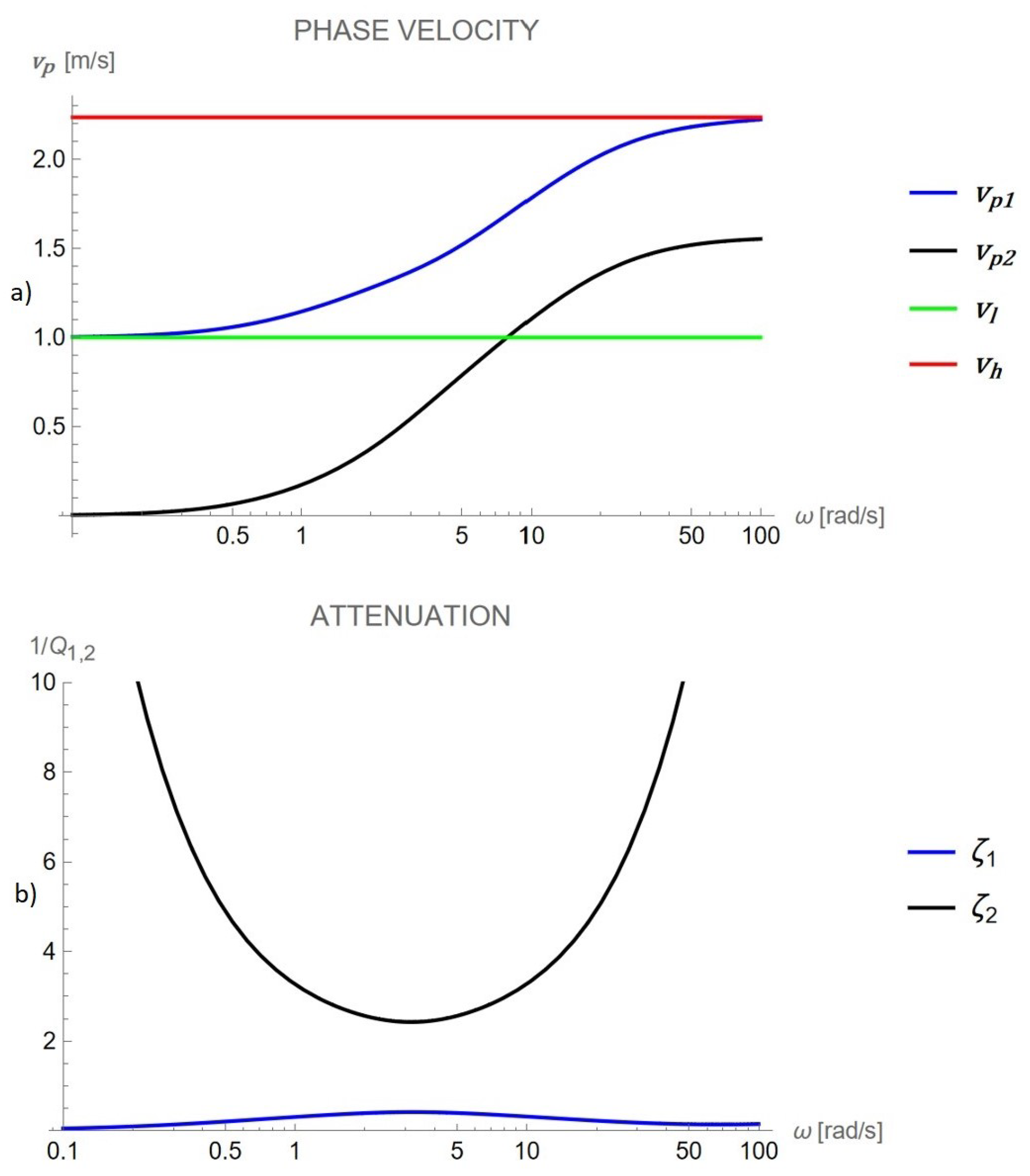
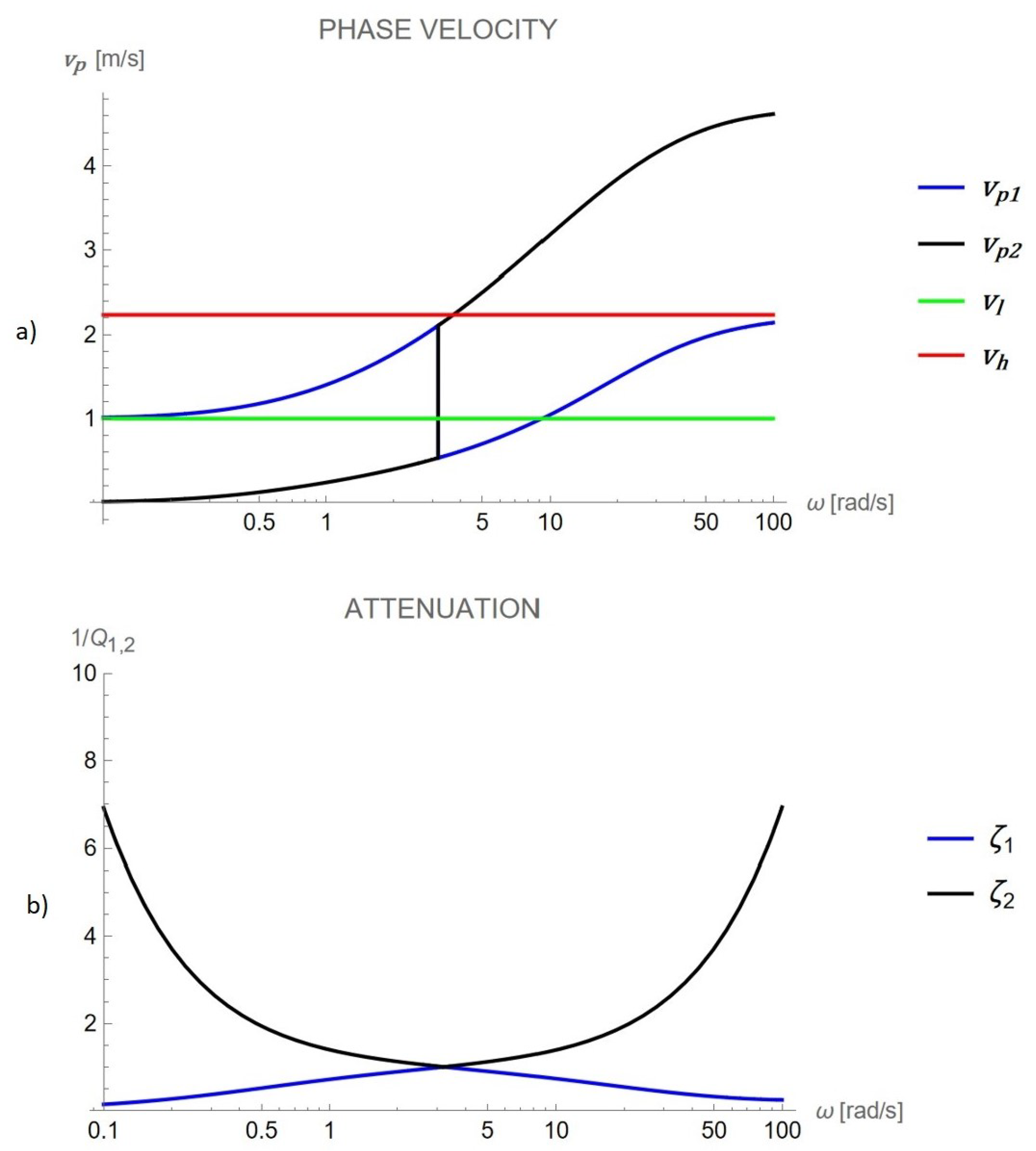
• Wave Dispersion: The analytical expression for the phase velocity (Equation (18)) reveals a frequency-dependent behavior with two distinct propagating modes. As frequency increases, the phase velocity transitions between two asymptotic regimes, consistent with experimental observations in complex structured materials.
• Wave Attenuation: Attenuation is described through the damping ratio $\zeta$ (Equation (19)), derived from the real and imaginary parts of the complex wave number. This parameter quantifies energy dissipation and reflects the influence of both first- and second-gradient viscosity.
• Characteristic Frequency: The model predicts a characteristic frequency at which attenuation peaks. This defines a transition zone between low-frequency (non-dispersive) and high-frequency (asymptotic) behavior.
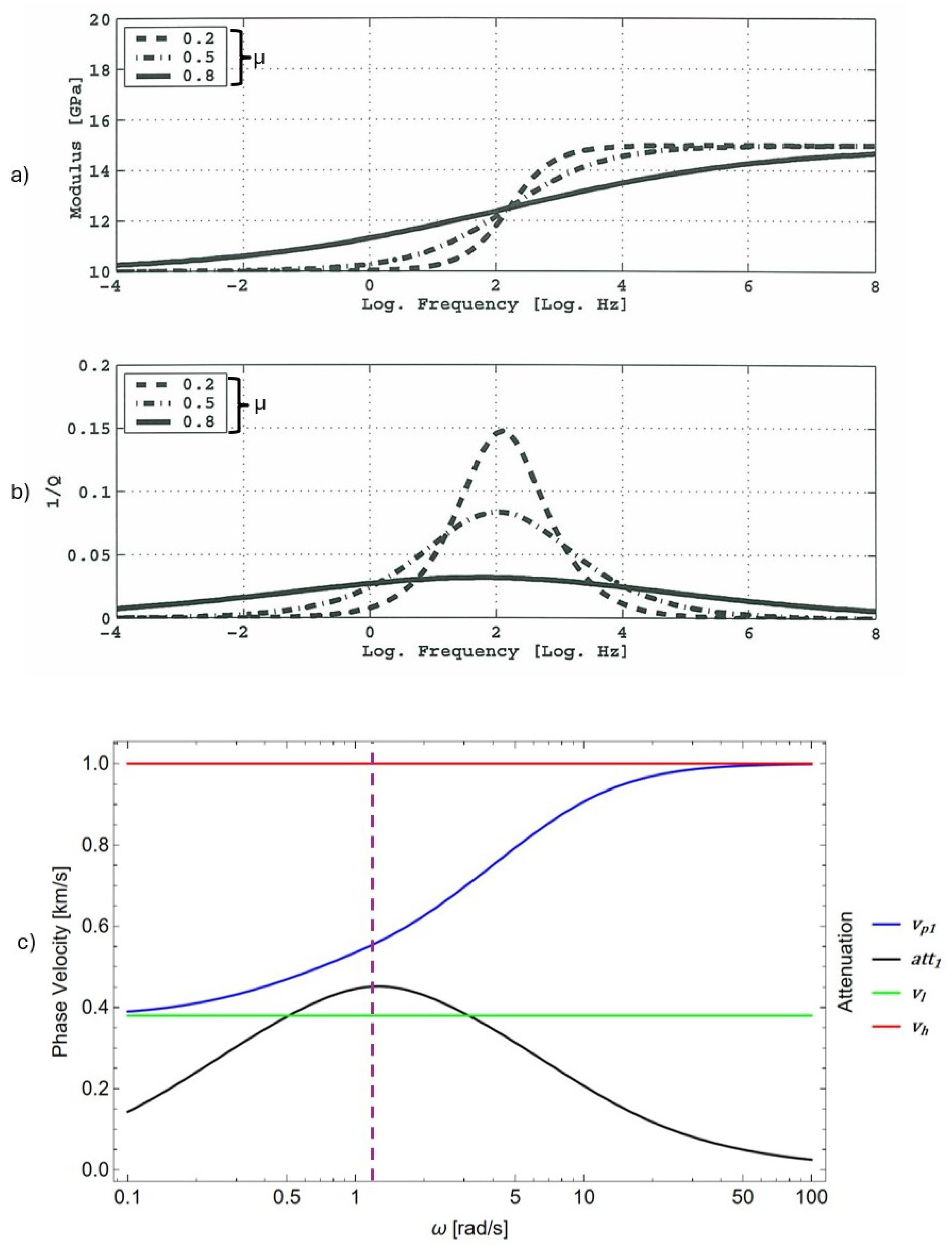
• Agreement with Literature: The model qualitatively reproduces trends in phase velocity and attenuation observed experimentally, notably those reported in Hofmann’s work (Figure 1), supporting the validity of the constitutive assumptions.
• Role of Higher-Order Effects: The inclusion of higher-order elastic ($k_2$) and viscous ($c_2$) terms introduces additional length and time scales, enhancing the model’s ability to capture the mechanical response of architectured or microstructured materials.

References

1. Aifantis, E.C. The Role of Gradient in the Mechanics of Materials. J. Elast. 2003, 72, 177–200. [Google Scholar]
2. dell’Isola, F.; Steigmann, D. A Two-Dimensional Gradient-Elasticity Theory for Woven Fabrics. J. Elast. 2015, 118, 113–125. [Google Scholar] [CrossRef]
3. Germain, P. The Mechanics of Materials with Second-Order Gradients. J. Mech. Phys. Solids 1973, 21, 489–509. [Google Scholar]
4. Eshelby, J.D. Elastic Inclusions and the Theory of Composite Materials. J. Elast. 1980, 10, 319–343. [Google Scholar]
5. Pendry, J.B. Metamaterials: The First Hundred Years. Science 2006, 314, 230–231. [Google Scholar]
6. Bauchau, P. Ultrasonic Wave Propagation in Biological Tissues. J. Acoust. Soc. Am. 2001, 110, 2417–2424. [Google Scholar]
7. Jafferis, J. Non-local Effects and Attenuation in Wave Propagation. J. Appl. Phys. 2015, 89, 283–299. [Google Scholar]
8. Lurie, D. Viscoelastic Effects in Second-Gradient Materials: A Theoretical Framework. J. Mech. Phys. Solids 2017, 102, 37–50. [Google Scholar] [CrossRef]
9. Bucur, D. Non-Destructive Testing of Materials by Ultrasonic Waves; Springer: Cham, Switzerland, 2010. [Google Scholar]
10. Hofmann, R. Frequency Dependent Elastic and Anelastic Properties of Clastic Rocks. Ph.D. Thesis, Colorado School of Mines, Golden, CO, USA, 2006; p. 185. [Google Scholar]
11. Lauwerier, H.A.; Koiter, W.T. North-Holland Series on Applied Mathematics and Mechanics. In North-Holland Series in Applied Mathematics and Mechanics; Elsevier: Amsterdam, The Netherlands, 1967; Volume 2. [Google Scholar]
12. Carcione, J.M. Wave Fields in Real Media: Wave Propagation in Anisotropic, Anelastic, Porous and Electromagnetic Media, 2nd ed.; Elsevier: Amsterdam, The Netherlands, 2007. [Google Scholar]
13. Lee, K.; Humphrey, V.; Kim, B.N.; Yoon, S. Frequency dependencies of phase velocity and attenuation coefficient in a water-saturated sandy sediment from 0.3 to 1.0 MHz. J. Acoust. Soc. Am. 2007, 121, 2553–2558. [Google Scholar] [CrossRef]
14. Philippidis, T.; Aggelis, D. Experimental study of wave dispersion and attenuation in concrete. Ultrasonics 2005, 43, 584–595. [Google Scholar] [CrossRef]
15. Mace, B.; Marconi, E. Wave motion and dispersion phenomena: Veering, locking and strong coupling effects. J. Acoust. Soc. Am. 2012, 131, 1015–1028. [Google Scholar] [CrossRef] [PubMed]
16. Rosi, G.; Giorgio, I.; Eremeyev, V.A. Propagation of linear compression waves through plane interfacial layers and mass adsorption in second gradient fluids. ZAMM-J. Appl. Math. Mech./Z. Angew. Math. Mech. 2013, 93, 914–927. [Google Scholar] [CrossRef]
17. Wolfenden, A. Dynamic Elastic Modulus Measurements in Materials; ASTM International: West Conshohocken, PA, USA, 1990. [Google Scholar]
18. Giorgio, I.; Della Corte, A.; Dell’Isola, F. Dynamics of 1D nonlinear pantographic continua. Nonlinear Dyn. 2017, 88, 21–31. [Google Scholar] [CrossRef]
19. Yang, B.; Bacciocchi, M.; Fantuzzi, N.; Luciano, R.; Fabbrocino, F. Computational simulation and acoustic analysis of two-dimensional nano-waveguides considering second strain gradient effects. Comput. Struct. 2024, 296, 107299. [Google Scholar] [CrossRef]
20. Yang, B.; Fantuzzi, N.; Bacciocchi, M.; Fabbrocino, F.; Mousavi, M. Nonlinear wave propagation in graphene incorporating second strain gradient theory. Thin-Walled Struct. 2024, 198, 111713. [Google Scholar] [CrossRef]
21. Laudato, M.; Barchiesi, E. Non-linear dynamics of pantographic fabrics: Modelling and numerical study. In Wave Dynamics, Mechanics and Physics of Microstructured Metamaterials: Theoretical and Experimental Methods; Springer: Cham, Switzerland, 2019; pp. 241–254. [Google Scholar]
22. Nejadsadeghi, N.; Misra, A. Role of Higher-order Inertia in Modulating Elastic Wave Dispersion in Materials with Granular Microstructure. Int. J. Mech. Sci. 2020, 185, 105867. [Google Scholar] [CrossRef]
23. Dell’Isola, F.; Madeo, A.; Placidi, L. Linear plane wave propagation and normal transmission and reflection at discontinuity surfaces in second gradient 3D continua. ZAMM-J. Appl. Math. Mech./Z. Angew. Math. Mech. 2012, 92, 52–71. [Google Scholar] [CrossRef]
24. dell’Isola, F.; Eugster, S.R.; Fedele, R.; Seppecher, P. Second-gradient continua: From Lagrangian to Eulerian and back. Math. Mech. Solids 2022, 27, 2715–2750. [Google Scholar] [CrossRef]
25. Shekarchizadeh, N.; Laudato, M.; Manzari, L.; Abali, B.E.; Giorgio, I.; Bersani, A.M. Parameter identification of a second-gradient model for the description of pantographic structures in dynamic regime. Z. Angew. Math. Phys. 2021, 72, 190. [Google Scholar] [CrossRef]
26. Giorgio, I.; Andreaus, U.; Dell’Isola, F.; Lekszycki, T. Viscous second gradient porous materials for bones reconstructed with bio-resorbable grafts. Extrem. Mech. Lett. 2017, 13, 141–147. [Google Scholar] [CrossRef]
27. Madeo, A.; Dell’Isola, F.; Darve, F. A continuum model for deformable, second gradient porous media partially saturated with compressible fluids. J. Mech. Phys. Solids 2013, 61, 2196–2211. [Google Scholar] [CrossRef]
28. Dell’Isola, F.; Hutter, K. Variations of porosity in a sheared pressurized layer of saturated soil induced by vertical drainage of water. Proc. R. Soc. Lond. Ser. A Math. Phys. Eng. Sci. 1999, 455, 2841–2860. [Google Scholar] [CrossRef]
29. Luciano, R.; Barbero, E. Formulas for the stiffness of composites with periodic microstructure. Int. J. Solids Struct. 1994, 31, 2933–2944. [Google Scholar] [CrossRef]
30. Fabbrocino, F.; Amendola, A. Discrete-to-continuum approaches to the mechanics of pentamode bearings. Compos. Struct. 2017, 167, 219–226. [Google Scholar] [CrossRef]
31. Abali, B.E.; Müller, W.H.; Dell’Isola, F. Theory and computation of higher gradient elasticity theories based on action principles. Arch. Appl. Mech. 2017, 87, 1495–1510. [Google Scholar] [CrossRef]
32. Romano, G.; Barretta, R.; Diaco, M. Genesis and progress of virtual power principle. Acta Mech. 2022, 233, 5431–5445. [Google Scholar] [CrossRef]
33. Ciallella, A.; Giorgio, I.; Eugster, S.R.; Rizzi, N.L.; dell’Isola, F. Generalized beam model for the analysis of wave propagation with a symmetric pattern of deformation in planar pantographic sheets. Wave Motion 2022, 113, 102986. [Google Scholar] [CrossRef]
34. Barchiesi, E.; Laudato, M.; Di Cosmo, F. Wave dispersion in non-linear pantographic beams. Mech. Res. Commun. 2018, 94, 128–132. [Google Scholar] [CrossRef]
35. Abali, B.E.; Vazic, B.; Newell, P. Influence of microstructure on size effect for metamaterials applied in composite structures. Mech. Res. Commun. 2022, 122, 103877. [Google Scholar] [CrossRef]
36. Migliaccio, G.; D’Annibale, F. On the role of different nonlinear damping forms in the dynamic behavior of the generalized Beck’s column. Nonlinear Dyn. 2024, 112, 13733–13750. [Google Scholar] [CrossRef]
37. Placidi, L.; Di Girolamo, F.; Fedele, R. Variational study of a Maxwell–Rayleigh-type finite length model for the preliminary design of a tensegrity chain with a tunable band gap. Mech. Res. Commun. 2024, 136, 104255. [Google Scholar] [CrossRef]
38. Berezovski, A.; Giorgio, I.; Corte, A.D. Interfaces in micromorphic materials: Wave transmission and reflection with numerical simulations. Math. Mech. Solids 2016, 21, 37–51. [Google Scholar] [CrossRef]
39. Placidi, L.; Rosi, G.; Giorgio, I.; Madeo, A. Reflection and transmission of plane waves at surfaces carrying material properties and embedded in second-gradient materials. Math. Mech. Solids 2014, 19, 555–578. [Google Scholar] [CrossRef]
40. Hima, N.; D’Annibale, F.; Dal Corso, F. Non-smooth dynamics of buckling based metainterfaces: Rocking-like motion and bifurcations. Int. J. Mech. Sci. 2023, 242, 108005. [Google Scholar] [CrossRef]
41. Varadan, V.K.; Varadan, V.V.; Ma, Y. Frequency-dependent elastic properties of rubberlike materials with a random distribution of voids. J. Acoust. Soc. Am. 1984, 76, 296–300. [Google Scholar] [CrossRef]
42. Romano, G.; Barretta, R.; Diaco, M. Spacetime evolutive equilibrium in Nonlinear Continuum Mechanics. Contin. Mech. Thermodyn. 2023, 35, 1859–1880. [Google Scholar] [CrossRef]
43. Greco, F.; Lonetti, P.; Pascuzzo, A.; Sansone, G. An Analysis of the Dynamic Behavior of Damaged Reinforced Concrete Bridges under Moving Vehicle Loads by Using the Moving Mesh Technique. Struct. Durab. Health Monit. 2023, 17, 457–483. [Google Scholar] [CrossRef]
44. Abali, B.E. Revealing the physical insight of a length-scale parameter in metamaterials by exploiting the variational formulation. Contin. Mech. Thermodyn. 2019, 31, 885–894. [Google Scholar] [CrossRef]
Figure 1. The influence of a certain parameter μ , as defined in Hofmann’s thesis [10], on phase velocity (a) and attenuation (b). The variation of phase velocity as a function of frequency is shown in (c), where a significant change occurs near the attenuation peak.
Civileng 06 00037 g001
Figure 2. Phase velocity v p (m/s) and damping ratio as functions of the frequency ω (rad/s) according to Equations (18) and (19) for a given material with constitutive parameters shown in Table 1. The characteristic frequency at which the attenuation peak occurs is 3.2 rad/s. The two asymptotes defined by Equations (20) and (21) are also shown.
Civileng 06 00037 g002
Figure 3. Phase velocity v p (m/s) and damping ratio as functions of the frequency ω (rad/s) according to Equation (18), subfigure (a), and (19), subfigure (b), for a given material with constitutive parameters as shown in Table 1. The point at which the velocity jump occurs corresponds to the common peak—respectively, maximum and minimum—of the two wave signals. The two asymptotes defined in Equations (20) and (21) are also represented in subfigure (a).
Civileng 06 00037 g003
Figure 4. Phase velocity v p (m/s) and attenuation coefficient α (dB/cm) as functions of the frequency ω (krad/s) according to Equation (18), subfigure (a), and (23), subfigure (b), for a sedimentary rock with constitutive parameters as shown in Table 1. Red points represent the experimental data from the literature [13] for phase velocity (subfigure (a)) and attenuation (subfigure (b)).
Civileng 06 00037 g004
Figure 5. Phase velocity v p (m/s) and attenuation coefficient α (dB/cm) as functions of frequency ω (krad/s), according to Equation (18), subfigure (a), and (23), subfigure (b), for a cement paste sample with constitutive parameters listed in Table 1. Red points represent the experimental data from the literature [14] for phase velocity (subfigure (a)) and attenuation (subfigure (b)).
Civileng 06 00037 g005
Figure 6. Phase velocity v p (m/s) and attenuation coefficient α (dB/cm) as functions of frequency ω (krad/s), according to Equation (18), subfigure (a), and (23), subfigure (b), for a concrete sample with constitutive parameters listed in Table 1. Red points represent the experimental data from the literature [14] for phase velocity (subfigure (a)) and attenuation (subfigure (b)).
Civileng 06 00037 g006aCivileng 06 00037 g006b