Article

Port-of-Entry Simulation Model for Potential Wait Time Reduction and Air Quality Improvement: A Case Study at the Gateway International Bridge in Brownsville, Texas, USA

1
Department of Civil Engineering, The University of Texas at Tyler, Tyler, TX 75799, USA
2
Department of Manufacturing and Industrial Engineering, The University of Texas Rio Grande Valley, Edinburg, TX 78541, USA
3
School of Earth, Environmental, and Marine Sciences, The University of Texas Rio Grande Valley, Brownsville, TX 78520, USA
*
Author to whom correspondence should be addressed.
CivilEng 2023, 4(1), 345-358; https://doi.org/10.3390/civileng4010020
Submission received: 20 December 2022 / Revised: 7 March 2023 / Accepted: 13 March 2023 / Published: 20 March 2023
(This article belongs to the Special Issue Next Generation Infrastructure)

Abstract

:
The mathematical study known as queueing theory has recently become a major point of interest for many government agencies and private companies for increasing efficiency. One such application is vehicle queueing at an international port-of-entry (POE). When queueing, fumes from idling vehicles negatively affect the overall health and well-being of the community, especially the U.S. Customs and Border Protection (CBP) agents that work at the POEs. As such, there is a need to analyze and optimize the border crossing queuing operations to minimize wait times and number of vehicles in the queue and, thus, reduce the vehicle emissions. For this research, the U.S.–Mexico POE located at The Gateway International Bridge in Brownsville, Texas, is used as a case study. Due to data privacy concerns, the hourly wait times for vehicles arriving at the border had to be extracted manually each day using a live wait time tracker online. The data extraction was performed for the month of March 2022. Using these wait times, a queueing simulation software, SIMIO, was used to develop an interactive simulation model and calibrate the service rates. The output from the SIMIO model was then used to develop an artificial neural network (ANN) to predict hourly particulate matter content with an R2 of 0.402. From the ANN, a predictive equation has been developed, which may be used by CBP to make operational decisions and improve the overall efficiency of this POE. Thus, lowering the average wait times and the emissions from idling vehicles in the queue.

1. Introduction

Queueing theory is one subdiscipline of operations research (OR), which examines each component of waiting in a line, including the arrival process, service process, and number of servers, among other performance measures [1,2,3]. In an application sense, queueing theory is observed via a check-out counter, vehicles at a toll booth, and even passengers at an airport checkpoint. As a subdiscipline of OR, the goal of queueing theory is to study the service lines or queues, in order to analyze and predict the time experienced by the entities across all operations, e.g., customers, vehicles, passengers, users, etc., with given constraints, e.g., number of servers, maximum service rates, etc. Queueing theory is, therefore, the preferred method to analyze systems with single or multiple queues and with single or multiple servers.
In the manufacturing or the service industry, queueing theory is used to evaluate and determine system performance measures. Once the current measures are determined, optimization and operational techniques are employed to improve the overall system performance. The system being analyzed is typically focused on a single operation or process at a time, where the line is formed from customers or products that need servicing or manufacturing. These entities wait in the queue to be serviced in a typically first-come, first-served fashion. The servicing operation is usually a machine or a server that provides the necessary activities for the entities in the line. Once the entity is served, it moves to the next server or queue for the next operation in the process. The entire time, the wait time plus service time, is typically what is reported as the time in the system.
Once such queueing theory application in recent years has been focused around improving the efficiency at ports-of-entry (POEs) between the U.S. and Mexico. The queueing model in this system consists of vehicles, i.e., passenger cars and commercial trucks, that form a line at the POE to be processed and inspected in order to go across the border and continue the journey of their goods.
The U.S. Customs and Border Protection (CPB) is part of the Department of Homeland Security (DHS), one of the world’s largest law enforcement organizations, and it is charged with keeping terrorists and their weapons out of the U.S., while facilitating lawful international travel and trade. The mission statement of CBP is to “protect the American people, safeguard our borders, and enhance the nation’s economic prosperity” [4]. As the United States’ first unified border entity, CBP’s main task is to control customs and border security.
Currently, vehicles native to Mexico that cross through a POE into the U.S. must meet federal Department of Transportation (DOT) regulations. The Federal Motor Carrier Safety Administration (FMCSA), under the DOT, is tasked with overseeing such regulations. According to the FMCSA, “A Mexico-domiciled motor carrier that enters the U.S. must have a US DOT number, FMCSA-assigned MX number, a valid FMCSA Certificate of Registration for commercial-zone operations, or long-haul Provisional or Standard Operating Authority Registration, regardless of the size/type of vehicle, distance traveled into the U.S. or frequency of trips” [5].
Once it is the turn of the commercial truck to go through the inspection booth, officers at the POE verify each vehicle’s documentation and cargo. A vehicle that fails to pass the primary inspection is subjected to secondary inspection. Figure 1 presents the layout of the checkpoint with one queue, two inspection lanes, and one secondary inspection lane.
A POE may be modeled as a queueing network, with each inspection officer as a server and one queue leading to the multiple servers. While the vehicles are queueing and waiting to be served, they are idling and releasing toxic gases into the surrounding air. The officers at each inspection lane shoulder a substantial exposure burden of various criterial air pollutants, such as atmospheric particulate matter (PM), that have a diameter of less than 2.5 μm (PM2.5), nitrogen dioxide (NO2), and toxic gaseous pollutants, such as benzene, toluene, and xylenes [6,7]. This can have severe health implications for the federal officers, in terms of high asthma rates, hypertension, and various cardiovascular health effects [7]. Since the majority of commercial trucks are diesel engines, some research also has been performed to study the feasibility of additional filters, including biofilters, to reduce pollutant emissions [8]. Additionally, some vehicles may require secondary inspection, which increases the service time and CBP resources (i.e., more inspection officers).
The efficiency of a POE can be measured by the average time spent by vehicles in the queue (i.e., the waiting time to be served), which is dependent on the number of inspection officers (or servers). The emissions from idling vehicles in the queue may be correlated to health risks, namely for the inspection officers.
This research focuses on the Gateway International Bridge (GIB) border crossing in Brownsville, Texas, as a case study. In particular, the following research questions will be answered in this paper:
  • Research Question 1 (RQ1): Can readily available online border crossing wait time data be used to predict the arrival rate of passenger vehicles at a border crossing?
  • Research Question 2 (RQ2): If the answer to RQ1 is “yes,” can a dynamic discrete event simulation model be developed in order to calibrate the service rates at a border crossing?
  • Research Question 3 (RQ3): If the answer to RQ2 is “yes,” can the simulation model’s predicted hourly wait time be used with other readily available parameters related to air quality, in order to predict the hourly particulate matter content (PM2.5)?
  • Research Question 4 (RQ4): How can the answers to the above research questions be used to construct a POE’s work schedule, so that enough inspection lanes are open in order to maintain the level of emissions to be below a baseline?
The answer to RQ1 will be the hourly arrival rates at the GIB border crossing for a one-month period to be used in a baseline simulation model. The answer to RQ2 will be the calibrated average service rates of the servers at the GIB border crossing for the simulation model. The answer to RQ3 will be a machine learning regression model, which makes use of the simulation model output from RQ2, as well as readily available air quality parameters, so that CBP may predict the air quality, with respect to the border crossing operational performance (i.e., wait time). In the future, sensors may be deployed to detect vehicle arrivals to a POE, so that CBP may then determine the number of inspection officers (i.e., servers) needed in order to stay below the desired emission baseline.
This article is organized as follows. After this introduction, issues related to modeling POE operations and applied machine learning techniques are reviewed. This is followed by a description of the simulation model, data, and machine learning models, specifically as it relates to answering the research questions. This paper concludes by highlighting the findings, limitations, and future research.

2. Review of the Problem and Related Works

2.1. POE Applications

The literature reviewed in this section provides an overview of queueing theory related to border crossing applications, but because there are many types of lines, queuing theory has applications in many areas. The types of lines include stationary, transient, deterministic, and stochastic, among others. Stationary queueing networks have been studied extensively in transportation systems [9,10,11,12]. Examples of studies in transient queueing systems have been explored in hospital systems [13]. However, the type of queueing systems observed at the POEs are very specific and typically stochastic, non-stationary, and time-dependent systems.
To address these modeling challenges of the POE and evaluate the effects of security policies and procedures from CBP, research evaluating deterministic equivalent models has been performed [12]. The policies and procedures that CBP implements is also a significant consideration for commercial trucks and enterprises. Research in this area has shown that the companies consider the wait times at the POE when making decisions, and these decisions affect companies’ operations and logistics when moving goods across the border [14]. Other research has also reported on the high economic impact of delays on cross-border supply chains [15]. Finally, the use of block chains has also been attempted to assess the challenges and opportunities of the border trade [16]. Coyle et al. [17] studied the effects of POE policies and operations in logistics south of the border, and it affected Mexican practices. Olvera et al. [18] studied ultrafine particle levels at another POE between the US and Mexico in El Paso, Texas. Although particle analysis and wait times have been studied at POE’s at the sea-port-gate-yard interface [19,20] and emission reduction methods have been studied in the past [21], to our knowledge, no research has incorporated particle analysis and border wait times in the decision-making models; however, more research needs to be performed.

2.2. Machine Learning Techniques

The literature reviewed in this section is related to the machine learning techniques. In this research, several supervised regression machine learning techniques are applied to answer RQ3. Linear regression is one of the most well-known algorithms used in supervised machine learning. More complex machine learning algorithms include decision trees, support vector machines, random forest, and artificial neural networks (ANNs). ANNs are highly interconnected networks that have robust computational and pattern recognition capabilities [22]. This machine learning technique has been widely used due to its ability to model non-linear relationships in a non-complex way. ANNs were originally developed to emulate the human brain, which has led to a growing usage of ANNs in the engineering field for numerical and statistical methods, in lieu of traditional linear regression. In general, a three-layer feed-forward backpropagation ANN with a sigmoid activation function and one hidden layer is the most common type of ANN [22]. In addition, one hidden layer is typically sufficient for solving most of the non-linear problems without network overfitting [22].

3. Methodology

3.1. Discrete Event Simulation Model

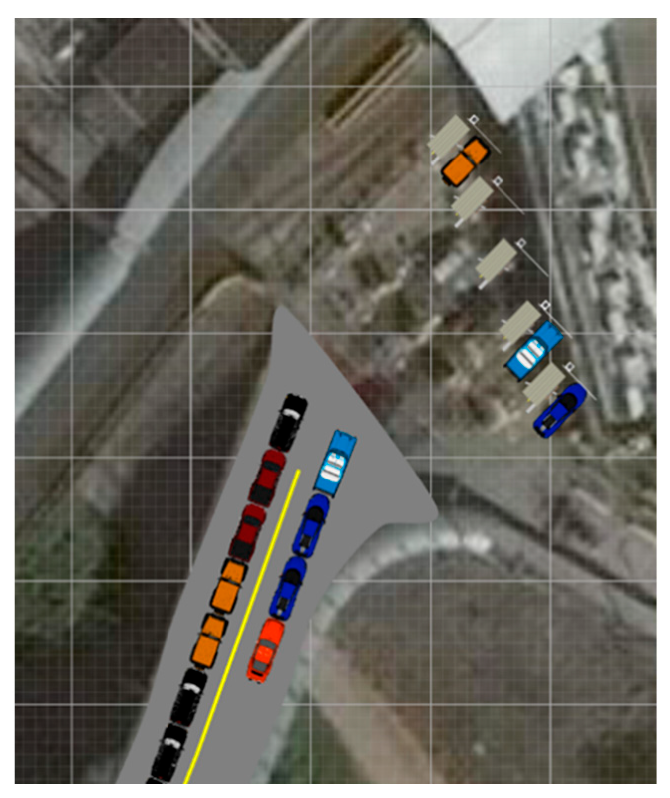
For this research, the Gateway International Border (GIB) POE in Brownsville, TX, was used as a case study. The first step was to develop a discrete event simulation model of the POE using SIMIO [23]. The POE consists of two lanes, which lead to five checkpoints (i.e., servers). Each checkpoint may be open or closed at hourly intervals. The overall footprint of the model within SIMIO was drawn to scale by importing a map of the border crossing using a geographic information system (GIS) [24]. Figure 2 presents the placement of the five checkpoints, some online with vehicles being served and others offline (i.e., no officer at the booth). The two lanes on the bottom portion of the figure are vehicles from Mexico waiting to be served before entering the U.S.
Most vehicle POE locations have three different levels of designated lanes available for travelers: general lanes, ready lanes, and Secure Electronic Network for Travelers Rapid Inspection (SENTRI) lanes. Anyone can use the general lanes, but it should be noted that the service rates are typically lower than other lanes. Ready lanes are dedicated lanes for travelers crossing the border that possess identification containing a radio frequency identification (RFID) chip. The ready lanes are typically faster than the general lanes and are the most used lane at most border crossings [25]. SENTRI is a paid program offered by the U.S. CBP allowing for pre-approved, low-risk individuals to pay a premium for priority crossing privileges and expedited clearance when entering the U.S. The SENTRI program costs $122.25 for five years of access [26].
Available data for this research was very scarce. Since the POE is operated by the CBP, available information pertaining to wait times, service rates, and the number of vehicles passing through the border was very limited. Additionally, there was no SENTRI lane information available at all. As such, the SENTRI lanes were omitted from this study. The following data were collected and processed in the manner described below.
The average hourly wait times for the general lane and the ready lane for the month of March 2022 were collected and documented using information available online from CBP’s border wait time website [27]. The website provides the current wait time, in minutes, for each lane at the border. Unfortunately, the website resets each night at 12:00 A.M., and there is no way to recover data from a previous day. Therefore, screenshots were taken each day at 11:00 P.M. throughout the month of March 2022 to collect a full month’s worth of wait time data. The data were manually entered into a database with a total of 744 hourly wait time data points (31 days × 24 h/day).
Then, the total number of vehicles that passed through the border during the month of March 2022 was also documented [28]. However, this was an aggregated total number of vehicles for the month and was not at lane level accuracies, nor as an hourly rate of vehicles. As such, the hourly arrival rate of general and ready vehicles was estimated by using
A r r i v a l   R a t e t = w a i t   t i m e t t = 1 744 w a i t   t i m e s × t o t a l   n u m b e r   o f   v e h i c l e s
where
Arrival   Rate t = arrival rate of vehicles at time t ,   vehicles hour ;
wait   time t = hourly average wait time for a vehicle at time t ,   minutes ;
t = 1 744 wait   times = total wait time for all vehicles during study period minutes ;
total   number   of   vehicles = total number of vehicles during study period vehicles .
Additionally, there were several general assumptions that were made during the data processing. These assumptions were as follows:
  • The minimum arrival rate for the general lanes were 30 vehicles/hour.
  • The minimum arrival rate for the ready lanes were 45 vehicles/hour.
  • Ready lanes have service rates that are approximately 20% faster than the service rate of general lanes [25].
  • A total of 15% of the total number of vehicles passing through the border were SENTRI level vehicles and were, thus, excluded from the usable data [26].
These assumptions were made for a number of reasons. The main reason being that the amount of available data pertaining to border crossing statistics was very limited. As such, these assumptions were made using deductive reasoning given the available data. The hourly arrival rates were then entered into SIMIO assuming a random Poisson distribution (i.e., an exponential interarrival time).
Once the hourly arrival rate was estimated and entered into SIMIO, the service rates for the general and ready passenger vehicles needed to be calibrated. This was performed simply by trial and error, as the ready lane service rates have a direct relationship with the service rate of the general lanes (i.e., 20% faster) [25]. Therefore, both service rates could be updated by trial and error until the SIMIO model’s overall total wait time matched the actual total wait time for the entire study period. The SIMIO model included the number of vehicles moving through the general and ready lanes each hour, the number of general and ready lanes opened during each hour, and the hourly schedule for the month of March 2022. SIMIO could add or remove active servers at hourly intervals. The calibrated service rates for the general and ready lanes were 11.5 s/vehicle and 9.0 s/vehicle, respectively. A summary of the calibration values is presented in Table 1.
The general lane and ready lane service rates were adjusted and calibrated, such that the SIMIO model’s total output of 40,566 min was the same as the actual total wait time of 40,691 min for the GIB during the month of March 2022.

3.2. Development of Models to Predict PM2.5

Once the SIMIO model was calibrated to accurately predict the average wait time in the queue, average wait time in the system, average number of vehicles in the queue, and average number of vehicles in the system at each hour, the next step was to make use of the SIMIO model’s predicted output of the hourly average wait time for a vehicle entering the queue, as well as other air quality parameters, in order to predict the amount of emissions created by idling (i.e., queueing) vehicles at the GIB POE. In addition to the hourly wait time, the hourly relative humidity, hourly temperature, and hourly wind speed were used as the four input parameters to predict PM 2.5 content at the GIB POE. The function follows the form:
P M 2.5 = f w a i t   t i m e ,   r e l a t i v e   h u m i d i t y ,   t e m p e r a t u r e ,   a n d   w i n d   s p e e d  
where
  • PM 2.5 = amount of inhalable pollutant particles in the air at hour t   micrograms meter 3 ;
  • wait   time = average wait time for a vehicle entering the queue at hour t   minutes ;
  • relative   humidity = average relative humidity of the air at hour t   percentage ;
  • temperature = average air temperature at hour t   degrees   Fahrenheit ;
  • wind   speed = average wind speed at hour t   mph .
The average wait time for a vehicle entering the queue was obtained directly from the SIMIO model at hour t . The average relative humidity, average air temperature, and average wind speed was gathered from [29] for each hour, t , during the entire month of March 2022. Equipment located at the Brownsville South Padre Island International Airport was used to collect these data [29].
The number of inhalable pollutants in the air was collected near the GIB POE location using BlueSky Low-Cost Sensors (Model: 8143 by TSI Inc., Shoreview, MN, USA) [30]. The BlueSky sensor was located approximately 0.04 miles from the GIB POE. This instrumentation is easy to install and weighs about 0.35 lb. The sensor does not require much power, approximately less than 5W (5 VDC @ 1 Amp). The PM sensor included is pre-calibrated similarly to other high-quality TSI equipment, such as the DustTrak™ models (TSI Inc., Shoreview, MN, USA). Self-diagnostic tests are configured to daily cleaning intervals to attain high-quality data. The PM sensor measures from the range 0 to 1000 μg/m3, with a measurement resolution of 1 μg/m3 and a response time being 1 s [30]. For this study, the particulate matter readings were collected every hour for the entire study period.
Extensive quality assurance and quality control (QA and QC) studies, conducted by the South Coast Air Quality Management District (South Coast AQMD) on BlueSky sensors, have shown a good record of performance and evaluations, with the sensors showing a moderate to strong PM2.5 (0.66 < R2 < 0.78) correlation with other federal equivalent method (FEM) instruments, such as FEM GRIMM and FEM Teledyne API T640, in the field [31].
The descriptive statistics for the data that was collected is presented in Table 2.
Based on the results presented in Table 2, some of the parameters from the dataset had a large range of values. For example, the number of minutes waited by vehicles ranged from 0 to 270 min, depending on the time of day and the number of servers that were open. This resulted in a standard deviation of 45.6 min. Likewise, the other parameters also varied widely, thus resulting in a rather complex dataset.
The next step was to develop a predictive model, which may be used by CBP, in order to predict the number of inhalable pollutants in the air near the GIB POE. Two common machine learning models were considered: a simple linear regression model and a more complex, non-linear ANN model.
The first model was a simple linear regression model, as it is the most common and simple machine learning technique, due to the interpretability of the results. The multiple linear regression results from this study are presented in Table 3.
As presented in Table 3, the intercept, relative humidity, and temperature parameters were all very statistically significant. The wind speed parameter was not very statistically significant, but with a positive coefficient, as expected. On the other hand, the wait time parameter, directly taken from the calibrated SIMIO model, was not statistically significant and had a negative coefficient, which is counterintuitive. It is expected that, as the wait time at the GIB POE increases, the PM 2.5 content should increase, as well. This could be one of the reasons for the low R2 value for the linear regression model of only 0.216. As such, a more complex machine learning algorithm, known as an artificial neural network (ANN), was used to create a more accurate model.
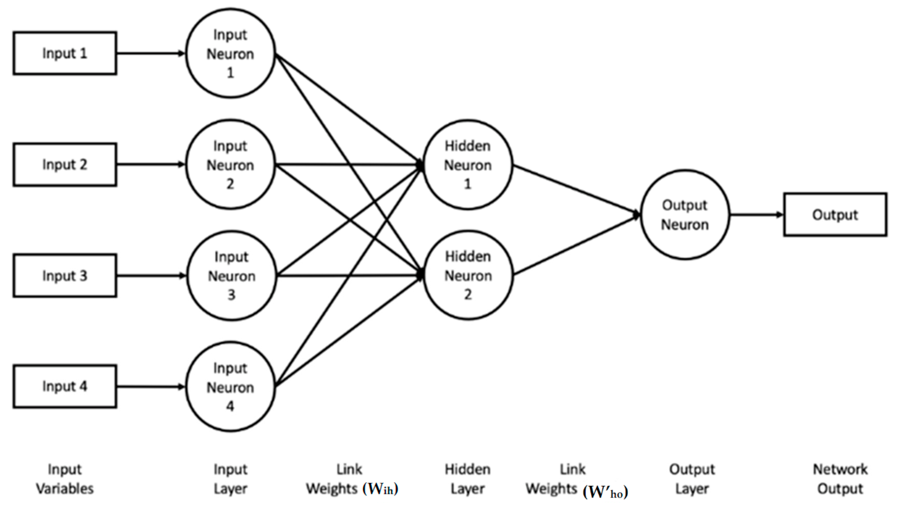
The second model was an ANN. A three-layer, feed-forward backpropagation ANN with a sigmoid activation function and one hidden layer is the most common type of neural network [22]. In addition, one hidden layer is typically sufficient for solving most of the non-linear problems without network overfitting [22]. For the purpose of this study, a three-layer, feed-forward neural network, with a hyperbolic tangent activation function, a backpropagation-error calculation algorithm, and two neurons in the hidden layer, was utilized using MATLAB [32]. Figure 3 demonstrates the utilized network architecture for the study, and its main components may be summarized as follows:
(1)
Input layer (i) with four input neurons, one neuron for each independent input parameter (see Equation (2) and Table 2).
(2)
Weight factors (Wih) between the input layer (i) and the hidden layer (h). The weight matrix contained 8 different values, one value from each input to each hidden layer neuron.
(3)
Hidden layer (h) with two hidden neurons having a tan-sigmoid activation function and two biases values (bhi).
(4)
Weight factors (W’ho) between the hidden layer and the output layer. The weight matrix contained two values, one value from each hidden neuron to the output neuron.
(5)
Output layer (o) with one output neuron for the dependent variable having a linear transfer function and single-bias value (Bo).
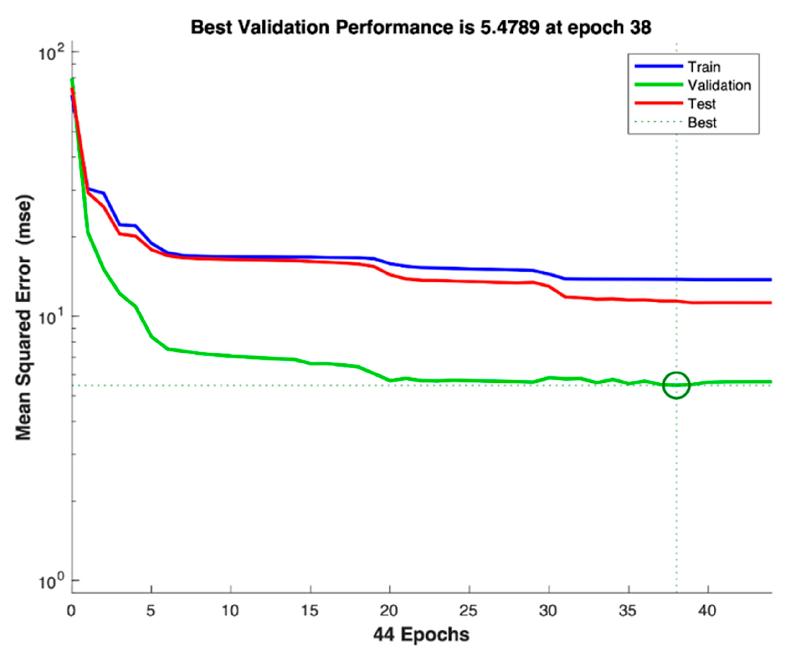
Before feeding into the network, each input variable was normalized to fall within the range [−1, 1]. Additionally, the output neuron predicts the normalized output, which also falls within the range of [−1, 1]. The output from the output neuron is then denormalized, so that the predicted PM2.5 value falls within an acceptable range (see Table 2 for minimum and maximum values). The training was conducted utilizing the Levenberg–Marquardt backpropagation algorithm in MATLAB [32]. This training algorithm divides the data into three categories. A total of 70% of the data were randomly utilized for training the model, while the remaining 30% of the data were divided into model testing and validation data sets. The ANN model was developed using only the training data. The testing and validation data were unseen to the developed ANN model. As shown in Figure 4, as an effort to avoid overfitting and maintain network generalization, the training was stopped when the validation dataset root mean square error stopped decreasing [22,32].
The developed model was trained utilizing the extracted 744 data points in MATLAB [32] by feeding the four input parameters in the input layer. Several ANN’s were trained with fewer hidden layer neurons; however, the model results were unsatisfactory. The number of hidden layer neurons was gradually increased until the ANN achieved satisfactory results. The idea was, by using the minimal number of hidden layer neurons, the ANN and stand-alone equation (which will be discussed in a subsequent section) may be made as simple as possible. The final ANN architecture had only two hidden layer neurons.
The model performance was evaluated in MATLAB, as shown in Figure 5, which demonstrates the ability of the model in the prediction of PM 2.5 . The ANN model yielded a relatively low coefficient of determination (R2) of 0.402 for the entire dataset (i.e., training, testing, and validation data). This means that the data possesses a high variability around the regression line, as presented in Figure 5.
Based on the results presented in Figure 5, the ANN model underpredicts the PM2.5 content in all four datasets. The validation set yielded the highest R2 value. The overall dataset graph, being the entire dataset of all 744 data points, yielded an R2 value of 0.402. As such, using the ANN model developed here, it can be seen that the R2 value of the ANN model was almost double the R2 value of the simple linear regression, which had an R2 value of only 0.216.

3.3. Extracted ANN Equation to Predict PM2.5

Despite the fact that ANN is a reliable tool for analysis and data classification, many researchers considered it a black box, due to their inability to have a clear understanding of what is happening inside the model. Essentially, inside the model, first each input variable is normalized to fall within the range of [−1, 1]. This is recommended for most ANN’s developed, so that the link weights and biases do not become very small [22]. Utilizing the minimum and maximum values in Table 2, each variable is normalized to fall within the range of [−1, 1].
Then, the normalized input variables are then multiplied by the link weights to both of the hidden layer neurons. Therefore, both hidden layer neurons have an input of each normalized input variable multiplied by its respective link weight. The bias for each hidden layer neuron is then added to the equation to obtain one final input value to each hidden layer neuron. Next, the hyperbolic tangent activation function is used to truncate each hidden layer’s output to fall within the range of [−1, 1]. Each hidden layer output is then multiplied by its respective weight to the single output neuron. The output neuron receives the output from each hidden layer multiplied by its respective link weight, as well as a bias term. This produces the normalized output, which falls within the range of [−1, 1]. This is because the input variables used also fell within the range of [−1, 1] when normalized. The output neuron value is then denormalized, so that it falls within the correct range for the predicted PM2.5 (see Table 2 for the minimum and maximum ranges).
From the utilized ANN structure, as shown in Figure 3, it can be concluded that the weights from the input layer to the hidden layer, the bias values in the hidden layer, the weights from the hidden layer to the output layer, and the bias values in the output layer are needed to extract a stand-alone equation from the trained ANN network. The values of the weights and biases are emphasized below, as extracted from MATLAB [32].
W ih =   0.079 0.721 0.041 0.848 1.962   27.346   47.696   0.344 W ho   = 0.139 0.170 b ih   = 0.726 15.501 b ho   = 0.675
Using these link weights, the following extracted equation was developed as a way of representing the ANN model in the form of an equation. This was performed so that the ANN model may be used by anyone outside the MATLAB environment. This equation also allows for future data points to be used in predicting new outputs.
ANN Output = 2.7006265 tanh(0.00058a + 0.01862b − 0.00125c − 0.04138d − 0.75637)
+ 3.3024915 tanh(−0.01453a + 0.70643b + 1.46778c + 0.01677d − 165.14774) + 7.3079335
where
ANN   Output = predicted output from ANN model of inhalable pollutant particles in the air μ g meter 3 ;
  • a = average wait time for a vehicle entering the queue at hour t   minutes ;
  • b = average relative humidity of the air at hour t   percentage ;
  • c = average air temperature at hour t   degrees   Fahrenheit ;
  • d = average wind speed at hour t   mph .
The generated stand-alone equation yields the same output as the ANN. Furthermore, it should be noted that, in order to use Equation (3), the input parameters should fall within the [min, max] range, as presented in Table 2. In Equation (3), the two neurons may be seen, each of which use the hyperbolic tangent activation function. The coefficients to both hidden layer neurons are the link weights from the hidden layer to the output layer, and the bias from the output layer may also be seen in the stand-alone equation. The coefficient and bias to the entire equation are used to denormalize the output from the output neuron to fall within the correct range for an acceptable PM2.5 prediction.

4. Results and Discussions

4.1. Research Question 1

The first research question asked if readily available online border crossing wait time data may be used to predict the arrival rate of vehicles at a border crossing. The answer to this research question is “yes.” Readily available wait time data and aggregated total vehicle data were gathered online from [27,28] to estimate the hourly arrival rate of vehicles at a border crossing using Equation (1). For this research, the GIB POE in Brownsville, Texas, was used as a case study.

4.2. Research Question 2

The second research question asked, if the answer to RQ1 is “yes,” can a dynamic discrete event simulation model be developed in order to calibrate the service rate at a border crossing. The answer to this research question is also “yes.” Using the estimated hourly arrival rates from RQ1, SIMIO [23] was used to calibrate the general and ready lane service rates, such that the SIMIO model’s total predicted wait time for the entire month of March 22 was the same as the actual total wait time during the same month (see Table 1). The calibrated service rates for the general and ready lanes were 11.5 s/vehicle and 9.0 s/vehicle, respectively.

4.3. Research Question 3

The third research question asked, if the answer to RQ2 is “yes,” can the simulation model’s predicted hourly wait time be used with other readily available parameters related to air quality in order to predict the hourly particulate matter content PM2.5. The answer to this research question is also “yes.” Once the SIMIO model was calibrated as part of RQ2, the hourly wait times for the month of March 2022 were used in conjunction with the average hourly relative humidity, average hourly air temperature, and average hourly wind speed to predict the number of inhalable pollutants in the air near the GIB POE location. This was performed using a simple multiple linear regression model, as well as a more complex, non-linear ANN model. Because the ANN results, with an R2 = 0.402, were greater than the simple multiple linear regression model, an equation was extracted from the ANN, so that it may easily be used by CBP officials to predict the number of inhalable pollutants in the air near the GIB POE location. This was presented as Equation (3).

4.4. Research Question 4

The fourth research question asked if the answers to the above research questions can be used to construct a POE’s work schedule, so that enough inspection lanes are open in order to maintain the level of emissions to be below a baseline. The answer to this research question is also “yes.” Because a relationship between the ambient air properties and vehicle wait time at the GIB POE has been established, CBP officials may now construct a work schedule using the SIMIO discrete simulation model and Equation (3), both presented as part of this paper, in order to minimize the number of inhalable pollutants in the air near the GIB POE location.

5. Conclusions

5.1. Major Findings and Recommendations

The overall objective of this research was to demonstrate a clear correlation between long vehicle queueing times, as well as the number of emissions and hydrocarbon particles found in the air at these congested POEs. By analyzing the daily traffic patterns and improving the overall efficiency of certain border crossings, such as the one examined in this research, the number of emissions from idling vehicles in the queue could be significantly decreased, which may be correlated to certain health risks. Thus, optimizing and streamlining the border crossing process could prove to have major societal benefits, with regards to vehicle emissions and the health of the CBP agents.

5.2. Future Research

As with all research, there are limitations. One of the main limitations of this research is that the actual general and ready vehicle arrival rates were estimated based on limited, yet readily available, wait time data and aggregated vehicle crossing data online [27,28]. Access to data also limits the ability to accurately model POE operations, including secondary inspection, which is beyond the scope of this paper. In the future, actual general and ready vehicle arrival rates, as well as service rates, should be used in order to develop a queueing model, such as the one presented in this paper using SIMIO. Further sensitivity analysis could also be conducted to analyze the performance of the calibrated SIMIO model and extracted ANN equation under different scenarios at the GIB POE (e.g., very high arrival rates, less servers online, etc.) and at other POE’s. We recognize that raw data has homeland security implications and, thus, look forward to future research and collaboration with DHS and DOT.
Furthermore, the number of data points presented to the ANN model was very limited at only one month of data. By providing the model with more data points, the training, validation, and testing sets would all be larger, thus resulting in a more accurate model. Moreover, the addition of more hidden neurons into the ANN model could also potentially result in a more accurate model. Doing this usually results in a better R2 value; however, more hidden layer neurons result in a much longer extracted equation. With a more accurate simulation model and ANN equation, sensors may be deployed to detect vehicle arrivals at a POE, so that CBP may then determine the number of inspection officers (i.e., servers) needed in order to stay below the desired emission baseline.

Author Contributions

The authors confirm contribution to the paper as follows: study concept and design: B.S., M.V., H.M. and A.U.R.; literature review: B.S. and H.M.; data processing: B.S. and E.M.; analysis of results: B.S. and M.V.; initial draft of manuscript: B.S.; revisions of manuscript: M.V., H.M. and A.U.R. All authors have read and agreed to the published version of the manuscript.

Funding

This research received no external funding.

Institutional Review Board Statement

Not applicable.

Informed Consent Statement

Not applicable.

Data Availability Statement

Not applicable.

Acknowledgments

The research team would like to acknowledge and thank David Mendez for his assistance in the air quality data collection.

Conflicts of Interest

The authors declare no conflict of interest.

References

  1. Taha, H.A. Operations Research: An Introduction; Pearson/Prentice Hall: Upper Saddle River, NJ, USA, 2011; Volume 790. [Google Scholar]
  2. Winston, W.L. Operations Research: Applications and Algorithms; Cengage Learning: Boston, MA, USA, 2022. [Google Scholar]
  3. Jackson, J.R. Networks of Waiting Lines. Oper. Res. 1957, 5, 518–521. [Google Scholar] [CrossRef] [Green Version]
  4. About CBP, U.S. Customs and Border Protection, CBP 2021–2026 Strategy, An Official Website of the U.S. Department of Homeland Security. Available online: https://www.cbp.gov/about (accessed on 11 July 2022).
  5. Federal Motor Carrier Safety Administration, U.S. Department of Transportation. Available online: https://www.fmcsa.dot.gov/international-programs/cross-border-operating-requirements-mexico-domiciled-motor-carriers (accessed on 1 March 2022).
  6. Quintana, P.E.; Dumbauld, J.J.; Garnica, L. Traffic related Air Pollution in the community of San-Ysidro, CA in relation to northbound vehicle wait times at the U.S.-Mexico border Port of Entry. Atmos. Environ. 2014, 88, 353–361. [Google Scholar] [CrossRef]
  7. Spengler, J.; Lwebuga-Mukasa, J.; Vallarino, J.; Melly, S.; Chillrud, S.; Baker, J.; Minegishi, T. Air Toxics Exposure from Vehicle missions at a U.S. Border Crossing. Res. Rep. Health Effects Inst. 2021, 158, 5. [Google Scholar]
  8. Garcia, J.; Moya, H.; Lee, K.; Vargas, N. Feasibility of Biofilters to Reduce Pollutant Emissions in Diesel Engines. In Proceedings of the 2019 IISE Annual Conference, Orlando, FL, USA, 18–21 May 2019. [Google Scholar]
  9. Baskett, F.; Changdy, K.M.; Muntz, R.R.; Palacios, F.G. Open, closed and mixed networks of queues with different classes of customers. J. ACM 1975, 22, 248–260. [Google Scholar] [CrossRef]
  10. Neuts, M. Matrix Geometric Solutions in Stochastic Models: An Algorithmic Approach; Dover Publications: New York, NY, USA, 1981. [Google Scholar]
  11. Curry, G.L.; Feldman, R.M. Manufacturing Systems Modeling and Analysis; Springer: New York, NY, USA, 2009; pp. 85–97. [Google Scholar]
  12. Moya, H.; Rued, G. A Deterministic Equivalent Problem to Study the Effects of Security Policies. In Lecture Notes in Management and Industrial Engineering; Mula, J., Barbastefano, R., Díaz-Madroñero, M., Poler, R., Eds.; Springer: New York, NY, USA, 2018; Chapter 14; Volume 1, Available online: https://link.springer.com/book/10.1007%2F978-3-319-93488-4 (accessed on 11 July 2022).
  13. Curry, G.L.; Moya, H.; Erraguntla, M.; Banerjee, A. Transient queueing analysis for emergency hospital management. IISE Trans. Healthc. Syst. Eng. 2021, 12, 36–51. [Google Scholar] [CrossRef]
  14. Evaluating Cross-Border Logistics and Compliance at the US Texas Border. Available online: https://www.proquest.com/openview/6fc4c3f666d9ae259a5fbf1be069ac27/1?pq-origsite=gscholar&cbl=51908 (accessed on 11 July 2022).
  15. Cedillo-Campos, M.G.; Sánchez-Ramírez, C.; Vadali, S.; Villa, J.C.; Menezes, M.B. Supply chain dynamics and the “cross-border effect”: The US–Mexican border’s case. Comput. Ind. Eng. 2014, 72, 261–273. [Google Scholar] [CrossRef]
  16. Chang, Y.; Lakobou, E.; Shi, W. Blockchain in global supply chains and cross border trade: A critical synthesis of the state-of-the-art, challenges and opportunities. Int. J. Prod. Res. 2020, 58, 2082–2099. [Google Scholar] [CrossRef] [Green Version]
  17. Coyle, T.; Cruthirds, K.; Marques, B. World Class Logistics—South of the Border: An Analysis of Mexican Practices. Int. J. Prod. Qual. Manag. 2015, 15, 285–308. [Google Scholar]
  18. Olvera, H.A.; Lopez, M.; Guerrero, V.; Garcia, H.; Li, W.-W. Ultrafine particle levels at an international port of entry between the US and Mexico: Exposure implications for users, workers, and neighbors. J. Exp. Sci. Environ. Epidemiol. 2013, 23, 289–298. [Google Scholar] [CrossRef] [PubMed] [Green Version]
  19. Caballini, C.; Garcia, M.D.; Mar-Ortiz, J.; Sacone, S. A Combined Data Mining-Optimization Approach to Manage Trucks Operations in Container Terminals with the Use of a TAS: Application to an Italian and a Mexican Port. Transp. Res. Part E Logist. Transp. Rev. 2020, 142, 102054. [Google Scholar] [CrossRef]
  20. Iris, C.; Christensen, J.; Pacino, D.; Ropke, S. Flexible Ship Loading Problem with Transfer Vehicle Assignment and Scheduling. Transp. Res. Part B Methodol. 2018, 111, 113–134. [Google Scholar] [CrossRef] [Green Version]
  21. Iris, C.; Lam, J.S.L. A review of energy efficiency in ports: Operational strategies, technologies, and energy management systems. Renew. Sustain. Energy Rev. 2019, 112, 170–182. [Google Scholar] [CrossRef]
  22. Haykin, S.S. Neural Networks and Learning Machines, 3rd ed.; Prentice Hall/Pearson: Upper Saddle River, NJ, USA, 2009. [Google Scholar]
  23. Joines, J.A.; Roberts, S.D. Simulation Modeling with SIMIO: A Workbook; Simio, LLC: Pittsburgh, PA, USA, 2015. [Google Scholar]
  24. ESRI. Getting Started with ArcGIS; ESRI: Redlands, CA, USA, 2005. [Google Scholar]
  25. U.S. Customs and Border Protection. Ready Lanes. Available online: https://cbp.gov/travel/clearing-cbp/ready-lanes/ (accessed on 8 February 2022).
  26. U.S. Customs and Border Protection. SENTRI Lanes. Available online: https://cbp.gov/travel/trusted-traveler-programs/sentri/ (accessed on 8 February 2022).
  27. U.S. Customs and Border Protection. CBP Border Wait Times. Available online: https://bwt.cbp.gov/ (accessed on 1 March 2022).
  28. U.S. Department of Transportation Bureau of Transportation Statistics. Border Crossing/Entry Data. Available online: https://www.bts.gov/browse-statistical-products-and-data/border-crossing-data/border-crossingentry-data (accessed on 4 April 2022).
  29. Weather Underground, IBM Brownsville, TX, USA. Available online: https://wunderground.com (accessed on 1 March 2022).
  30. BlueSky Air Quality Monitor Operation and Maintenance Manual. TSI Inc.: Shoreview, MN, USA, 2021. Available online: https://tsi.com/getmedia/a9299d7b-de37-4177-ab3b-488dfbfd2d07/BlueSky_Op_Maint_Manual_6013929?ext=.pdf (accessed on 1 March 2022).
  31. AQMD Air Quality Sensor Performance Evaluation Center. 2021. Available online: http://www.aqmd.gov/aq-spec/evaluations/summary-pm (accessed on 1 March 2022).
  32. MATLAB and Statistics Toolbox; The Mathworks, Inc.: Natick, MA, USA, 2020; Available online: https://www.mathworks.com/products/statistics.html (accessed on 1 March 2022).
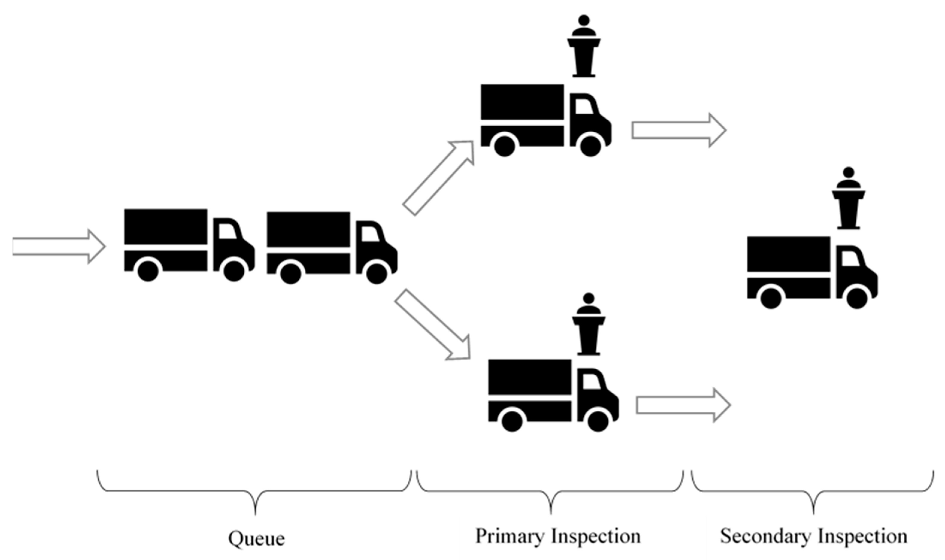
Figure 1. Layout of POE with two primary and one secondary inspection lanes.
Civileng 04 00020 g001
Figure 2. GIB POE in SIMIO [23].
Civileng 04 00020 g002
Figure 3. ANN Model Architecture.
Civileng 04 00020 g003
Figure 4. Number of iterations/epochs required for ANN model training.
Civileng 04 00020 g004
Figure 5. Predicted vs. Actual particulate matter quantity for ANN model for: (a) training; (b) validation; (c) test; and (d) all data.
Civileng 04 00020 g005
Table 1. Summary of the calibration values.
Available Online Data
Total No. of General Vehicles in March 2022 [28] 109 , 203   vehicles
Total No. of Ready Vehicles in March 2022 [28] 131 , 044   vehicles
Total No. of Minutes Waited [27] 40 , 691   min
Calibrated SIMIO Model Results
General Lane Calibrated Service Rate 11.5   seconds vehicle
Ready Lane Calibrated Service Rate 9.0   seconds vehicle
Total No. of Minutes Waited (SIMIO Model) 40 , 566   min
General Lane Average Arrival Rate 2.45   vehicles minute
Ready Lane Average Arrival Rate 2.94   vehicles minute
Table 2. Descriptive Statistics of Data Collected.
ParameterWait TimeRelative
Humidity
TemperatureWind SpeedPM2.5
Sample Size744744744744744
Units minutes % ° F mph μ g m 3
Min.010.047.001.0
Max.270.087.0112.041.040.0
Mean54.761.773.812.45.1
Std. Dev.45.620.612.17.84.5
Table 3. Linear Regression Results.
Input ParametersCoefficient t Statistics p Value
Intercept −10.3048−6.77772.4972 × 10−11
Wait   Time −0.0050−1.47950.1394
Relative   Humidity 0.121413.59839.4984 × 10−38
Temperature 0.10686.61107.3158 × 10−11
Wind   Speed 0.02241.08120.2800
R 2 0.2157
Observations744
Disclaimer/Publisher’s Note: The statements, opinions and data contained in all publications are solely those of the individual author(s) and contributor(s) and not of MDPI and/or the editor(s). MDPI and/or the editor(s) disclaim responsibility for any injury to people or property resulting from any ideas, methods, instructions or products referred to in the content.