Article

Predictive BIM with Integrated Bayesian Inference of Deterioration Models as a Four-Dimensional Decision Support Tool

by
Hendrik Morgenstern
* and
Michael Raupach
Institute for Building Materials Research, RWTH Aachen University, 52062 Aachen, Germany
*
Author to whom correspondence should be addressed.
CivilEng 2023, 4(1), 185-203; https://doi.org/10.3390/civileng4010012
Submission received: 12 December 2022 / Revised: 6 February 2023 / Accepted: 10 February 2023 / Published: 21 February 2023
(This article belongs to the Special Issue Next Generation Infrastructure)

Abstract

:
The durability of concrete structures is essential for reliable infrastructure. Although many deterioration models are available, they are rarely applied in situ. For existing structures in need of repair or durability assessment, this is also the case for Building Information Modeling (BIM). However, both BIM and durability modeling hold great potential to both minimize expended resources and maximize the reliability of structures. At the Institute for Building Materials Research (ibac) at RWTH Aachen University, a novel approach to the calibration of deterioration models using Bayesian inference iteratively in a BIM model enriched with machine-readable diagnosis data to achieve a predictive decision support tool is being developed. This paper demonstrates the digital workflow, validates the proposed approach, and expresses the added value for the planning of repair measures.

1. Introduction

As the need for reliable infrastructure steadily increases, the corresponding buildings progressively reach and exceed their service lives. To ensure safety nonetheless, the structures are kept under surveillance and are regularly diagnosed. If the need for action arises, there are several methods available to repair or strengthen the structures [1,2,3]. Besides conventional measures, innovative techniques are being developed and tested. For example, a multifunctional carbon-reinforced concrete interlayer called SMART-DECK allows moisture monitoring in real-time, preventive cathodic corrosion protection, and an increase in the shear force capacity [4]. Another example is given in [5], where strain and acceleration are monitored on a bridge and automatically analyzed to calculate a reliability index and assess the need for action. Although many monitoring systems and the generation of data itself are not considered new, automation and visualization via Building Information Modeling (BIM) are and thus, recent research focuses increasingly on these aspects of digitalization. That said, the presented paper intends to propose and demonstrate a novel way to analyze and visualize data in BIM. To support the comprehensibility of the presented research, the basics of BIM, digitalization in construction, deterioration modeling, and Bayesian statistics, as well as the different semantics, are explained below.

1.1. Digitalization in Construction

Although the construction sector is less advanced than most other sectors regarding digitalization, several innovative technologies have found application in recent years, arousing great interest and bringing new terminology with them such as BIM, the Internet of Things (IoT), and artificial intelligence (AI). A review of these tools and their usage in construction is given in [6], concluding that the enrichment of BIM models and the utilization of data are essential. Another review identifies insufficient software interoperability, limited BIM applications in operation and maintenance, a lack of application for transportation infrastructure, unclear economic benefits, and the difficulty of integrating BIM with other technologies as significant research gaps [7]. Pertaining to interoperability, an example of BIM usage for monitoring the maturity of concrete in a sensor-equipped formwork is given in [8]. BIM can also be combined with a bridge monitoring system (BMS) [9] or structural health monitoring (SHM), leading to structural health BIM (shBIM) [10]. Regarding enrichment, a BIM model can transition toward a digital twin (DT) or even digital twin construction (DTC) when it contains enough information and functionality [11,12]. Unlike a BIM model, a DT is expected to provide some kind of capacity to act [13]. To distinguish between the capabilities of different DTs, multiple BIM maturity levels are defined. The integration of inspection data or interactive real-time sensors in a DT leads to level 4 and if these data are used to predict future states or assist decision making, level 5 is achieved [14]. Most publications on DTs (30%) are related to facility management and the second most (24%) to SHM [15]. Examples of this are the enrichment of BIM with air temperature and carbon dioxide content [16] or power consumption and luminance [17]. However, the enrichment is always limited by the file format of the model and its ability to store and allocate information. The industry foundation classes (IFC) file format is standardized, transparent, and the most frequently used open-neutral format in BIM [18]. Although the IFC format ensures interoperability, its restrictions lead to significant research gaps in enriching IFC files regarding the optimization and management of (sensor) data [19]. Nonetheless, it is possible to enrich IFC files with diagnosis data. In previous publications, the IFC-compatible implementation of diagnosis data was presented [20,21,22].
In this publication, the focus is on BIM-based analysis and visualization of structural conditions, especially regarding automated calibration of deterioration models using the implemented data. To achieve this, a framework was developed using Revit (Autodesk) and the plugin Dynamo for visual programming. Visual programming, in contrast to conventional programming, provides a graphical user interface (GUI) and allows more intuitive programming and thus the user-friendly creation of scripts to implement data or automize processes in BIM. Dynamo is one of the most common tools used for visual programming in the construction sector (for more information on its usage refer to [23]).

1.2. Modeling and Probabilistic Analysis of Durability

Before calibrating a deterioration model with BIM-implemented diagnosis data, a deterioration model is required. There are several models available and still more to be developed for different applications and damage processes. The creation of a deterioration model for carbonation is demonstrated in [24]. Regarding the durability of infrastructure built with reinforced concrete, the corrosion of steel due to carbonation and/or chloride ingress may be relevant, whereas chloride ingress may be more critical in many cases. A review of empirical and electrochemical models for chloride-induced steel corrosion is given in [25]. Although most models consider only one damage process, the combination of chloride ingress and carbonation is often present in situ. As carbonation influences the pore structure and, ultimately, the chloride binding capacity of concrete, chloride ingress may be significantly higher in combination with carbonation [26,27,28,29]. However, the modeling of the combined damage processes is very complex [27] and only reliable under constant boundary conditions [30]. Although the combination of chloride ingress and carbonation is application-related, constant boundary conditions are not. Air humidity and temperature, however, are almost guaranteed to change over the year for most structures and influence the ionic transport [31] and the ingress of contaminations, respectively. Furthermore, there are often constraints to the models regarding the structure, as many models are only valid for uncracked concrete. Cracks accelerate ingress and lead to shorter periods for the initiation stage, which is why a correction factor is proposed in [32]. Additionally, most developed models are constrained to cementitious concrete and unsuited for concrete bound with alkali-activated materials (AAM). As the distribution of AAMs increases, new models are being developed [33] and already show deviating behavior regarding chloride ingress [34]. Given these influences, the validity and practicability of any deterioration model may seem questionable outside of the laboratory. For this reason, [35] proposes the calibration of existing models according to local characteristics, environmental influences, and diagnosis data rather than the creation of new models.
For both the creation and calibration of models, machine learning (ML), or rather artificial intelligence (AI), is increasingly being used. Although such methods are steadily gaining popularity, their practical application in the context of maintenance and repair is still subject to significant limitations. A review of AI identifies their overarching shortcoming as their lack of transparency, resulting in models that are less explainable and more difficult to improve [36]. This deficiency leads to less understanding and a lack of trust [37]. Especially in civil engineering, this can be seen as a major hurdle for practical application. In a comparison of different ML approaches for SHM, Bayesian inference or networks are identified as robust, simple, and generalizable, but with the disadvantage of large computational costs [38]. Another review of this topic emphasizes the rationality and comprehensibility of Bayesian methods [39].
The transparency, robustness, and simplicity of Bayesian inference have already led to versatile applications in civil engineering. From seismic models [40] and forecasts of climate [41] or project costs [42] to carbonation models [43], also in combination with chloride ingress [44], Bayesian inference is increasingly being used to calibrate models according to observations (diagnostic data) [45]. An application of Bayesian networks in reliability evaluation is given in [46], concluding their effectiveness while indicating their high computational expense. In short, Bayesian networks rely on Bayes’ theorem, given in Equation (1), which uses evidence B (e.g., knowledge of carbonation depth) to update/calibrate the probability of A (e.g., carbonation rate), given B.
P ( A | B ) = P ( B | A ) · P ( A ) P ( B )
P ( A | B ) : probability of A , given B P ( B | A ) : probability of B , given A P ( A ) : probability of A P ( B ) : probability of B
It should be noted that Bayes’ theorem uses probabilities and no metrics, often resulting from random distributions. If a distribution is assumed (a priori) but a very unlikely outcome is measured (evidence), the distribution can be updated accordingly (a posteriori). For further information on Bayesian inference, refer to [45,47,48]. This procedure of Bayesian inference can be automated and carried out in a software framework, which was previously performed to assess and update deterioration and reliability [49]. However, it will now be improved and implemented in BIM.

2. Data and Methods

2.1. Models, Assumptions, and Constraints

In this research, the deterioration models serve as fungible components in a BIM-based workflow. Two models from the fib Model Code for Service Life Design [50] are considered in the following, both for the initiation stage. One is for carbonation and the other is for chloride ingress. The model for carbonation is given in Equation (2). As the focus of the research is on BIM implementation and automated calibration, the model itself was simplified by assuming indoor conditions. The time of curing, as well as additional CO 2 emissions, were assumed to be unknown and thus taken out of the calculation. These assumptions can easily be overruled if required.
x c ( t ) = 2 · 1 R H i s 100 5 1 R H r e f 100 5 2.5 · k t · R A C C , 0 1 + ε t · C S , a t m · t
x c ( t ) : carbonation depth at time t [ mm ] R H i s : relative air humidity [ % ] R H r e f : relative reference air humidity [ % ] k t : regression parameter [ ] R A C C , 0 1 : inverse effective carbonation resistance of dry concrete , determined at time t 0 with the accelerated carbonation test method ACC [ ( mm 2 / a ) / ( kg / m 3 ) ] ε t : error term for the consideration of test-related errors [ ( mm 2 / a ) / ( kg / m 3 ) ] C S , a t m : CO 2 concentration of the atmosphere [ kg / m 3 ] t : time [ a ]
In the original description of the models, several layers of (sub)parameters are given. The more parameters that are involved, the more complicated and inefficient the Bayesian inference becomes. Therefore, models were consolidated to only contain parameters that should be updated. Furthermore, the boundaries for each parameter need to be given in order to limit the calculations and allow reasonable updates via Bayesian inference. The parameters that will be calibrated and their boundaries are given in Table 1.
For both carbonation and chloride ingress, some parameters are measurable, whereas others are empirically determined. Although the measurable parameters are not ultimately required to be updated and can even serve as evidence, the need for calibration of the incomprehensible parameters is even greater, as their influence can be significant while their values remain unvalidated. A popular discussion regarding this pertains to the age exponent a in the chloride model, as given in [51]. The model for chloride ingress is given in Equation (3) and the parameters that will be calibrated and their boundaries are given in Table 2.
C l ( x , t ) = C l Δ x · 1 erf x Δ x 2 · exp b e 1 T r e f 1 T i s · D R C M , 0 · t 0 t a · t
C l ( x , t ) : chloride content in depth x at time t [ wt % ] C l Δ x : chloride content in depth Δ x [ wt % ] erf : error term x : penetration depth [ mm ] Δ x : penetration depth deviating from Fick s behavior due to intermittent chloride input [ mm ] b e : regression parameter [ K ] T r e f : reference temperature [ K ] T i s : component temperature [ K ] D R C M , 0 : chloride migration coefficient of water-saturated concrete , determined at time t 0 with the test method RCM [ mm 2 / a ] t 0 : reference time [ a ] t : time [ a ] a : age exponent [ ]

2.2. Automation of Bayesian Inference

For the intended use case and the acceptance of this workflow, reasonable usability should be provided, which is why the Bayesian inference needs to be performed automatically and within minutes rather than hours. As the workflow is dependent on hardware and software, the used setup is defined as follows. The tests were carried out using the software shown in Table 3 and an Intel® Core i5-10400 CPU @ 2.90 GHz processor. Although different software was used to develop and validate the workflow, the results can be executed using only one piece of software (Revit). To achieve this, the functionality of the Bayesian network software GeNIe was integrated into Revit using PySMILE and Dynamo. The BIM implementation is demonstrated in the next section. First, the automation and acceleration of Bayesian inference are discussed, as these are vital requirements for feasible usage in BIM.
The practicability of the following workflow was an essential development target, namely that it should be suitable for ordinary computers and deliver good results in an appropriate processing time. As mentioned above [38,46], the processing time is the main disadvantage of Bayesian networks, which is why the implementation needs to be carried out proficiently. The two main settings influencing the processing time are the number of simulations (Monte Carlo method) and the number of bins for discretization. As Bayesian inference requires discrete probabilities and no continuous probability distributions, the parameters need to be discretized in several bins (sub-intervals). Each bin functions as an event and serves as input for Bayes’ theorem in Equation (1). To achieve good results, the bins need to cover the relevant intervals for both the a priori and a posteriori distributions in small increments. If the considered parameter has wide boundaries and/or is influential, many bins are required, leading to extensive processing times.
To accelerate the calibration process, an engineering approach was developed. Rather than dividing a broad interval into many bins, only a few bins should be used but for a narrowed-down interval. Thus, an algorithm was developed that iteratively performs Bayesian inference and shifts the boundaries of the parameters as long as certain criteria are (not) fulfilled. These criteria are adjustable at will. The following settings have proven to be effective. If a peripheral bin contains less than 1% of the sample, this bin is deleted, or rather, the interval bounds are narrowed down. If a peripheral bin contains less than 20% of the average (sample size/amount of bins/5), the boundaries are shifted toward the center of the bin, reducing the bin width by half. While the iteration continues, the probability distributions of the parameters are adjusted to fit the proposed probabilities resulting from the Bayesian inference and the nodes of the Bayesian network are re-discretized according to the new interval boundaries. This process is iterated until the deviations from the target value (evidence) are below a given value or if the iteration fails to narrow down the boundaries. The flowchart of the iterative inference process is shown in Figure 1.
For carbonation, the termination criteria are less than ±10% deviation from the mean and, if more than two pieces of evidence are given, less than ±30% deviation from the standard deviation. For chloride ingress, the termination criterion is less than ±20% deviation from the mean per-depth step. The process aborts if all depth steps fulfill this criterion. This allows for the quantification of the quality of the calibration, as well as a significant reduction in the processing time compared to the conventional Bayesian inference process, as discussed in Section 3.

2.3. Implementation in BIM

The Bayesian inference was implemented in BIM via Dynamo, Python, and PySMILE. Dynamo was used to access the objects of the BIM model including the implemented diagnosis data, perform geometric analyses, and run several Python scripts. The functionality of the Bayesian network software GeNIe was made available in Revit/Dynamo by importing the PySMILE library and using its functions in Python scripts. All functionalities were bundled into one Dynamo script containing 762 nodes, where many of the nodes were Python script nodes, adding even more layers, loops, and functions. As this Dynamo script is too complex to be discussed thoroughly in this paper, a compressed version is shown in Figure 2.
For further information and code samples, readers can refer to the upcoming dissertation of Hendrik Morgenstern, which will be published later this year by RWTH Aachen University. The Dynamo script for implementing Bayesian inference and reliability assessment in BIM requires the previous implementation of the diagnosis data published in [20,21,22]. Accordingly, certain objects for the diagnosis data need to be available in a machine-readable format, for example, multiple cylinders for drill dust probes carrying information about the chloride content in the respective depth as properties. Other than this, the BIM model does not need to meet specific requirements.
The script can be divided into three parts with the following subtasks:
A
Input
1
select components to be evaluated:
  • these components can be any objects with flat surfaces and do not need to be a certain object type;
  • there must be diagnosis data implemented in those objects for the script to run properly, as the calibration requires evidence;
  • all available evidence (diagnosis data) in these components will be combined into one sample.
2
select plane (can be any pickable object surface) as the reference for the z-axis;
3
geometries (such as width, height, etc.) of selected components are extracted;
4
previously implemented objects carrying the concrete cover (measured with linear scans during the building diagnosis) as properties available in the selected components are extracted;
5
previously implemented objects carrying the carbonation depths and chloride profiles as properties available in the selected components are extracted;
6
grouping of concrete cover in different rebar layers.
B
Analysis
1
Python environment with SMILE, the configuration of Bayesian networks (sample size, number of bins), and further input such as critical chloride threshold:
  • the user is required to define the values for certain configuration parameters via Dynamo as additional input if the default values are not used;
  • the user is required to navigate to the folder in which the Python environment with SMILE was installed so that Revit can add this folder to its system path and assess the functionality of SMILE.
2
monitoring data as a CSV data set, if available;
3
analysis of concrete cover (mean, standard deviation, quantiles);
4
Bayesian inference, using all available diagnosis data as evidence;
5
analysis of rebar location (eccentricity, tilting);
6
reliability assessment, including prognoses of carbonation and chloride ingress, as well as calculation of probabilities of failure (depassivation) and reliability indices;
7
assessment of repair methods.
C
Output
1
export of analysis results as CSV, TXT, XDSL;
2
creation of additional BIM objects (flat layers) hovering over the component surface containing the most relevant analysis data that are IFC compatible.
Fundamentally relevant to the process of calibrating models is the underlying evidence. As the workflow is implemented in BIM, it can not only read evidence but also allocate it in the 3D model. Thus, the program can be configured to only consider the evidence (A5) from certain elements (A1) at a certain distance (A2). For example, it can only consider chloride profiles in columns below 0.5 m measured from the floor. That said, monitoring systems (B2) can be implemented in BIM and also used as evidence input. The Bayesian inference (B4) uses all available evidence and saves the Bayesian networks as XDSL files for each iteration, allowing maximum transparency and the possibility of later examining the networks in GeNIe. The results of the various analyses (B3, B5, B6, B7) are exported in several file formats (C1) and stored in an additionally created object (C2). Thus, the original BIM model does not have to be suitable for this enrichment in any particular way. The only requirement is the availability of the diagnosis data, which has to be provided as specific objects. For more information on these BIM-implemented diagnostic data, readers can refer to [20,21,22].

3. Results

3.1. Calibration of Carbonation Model

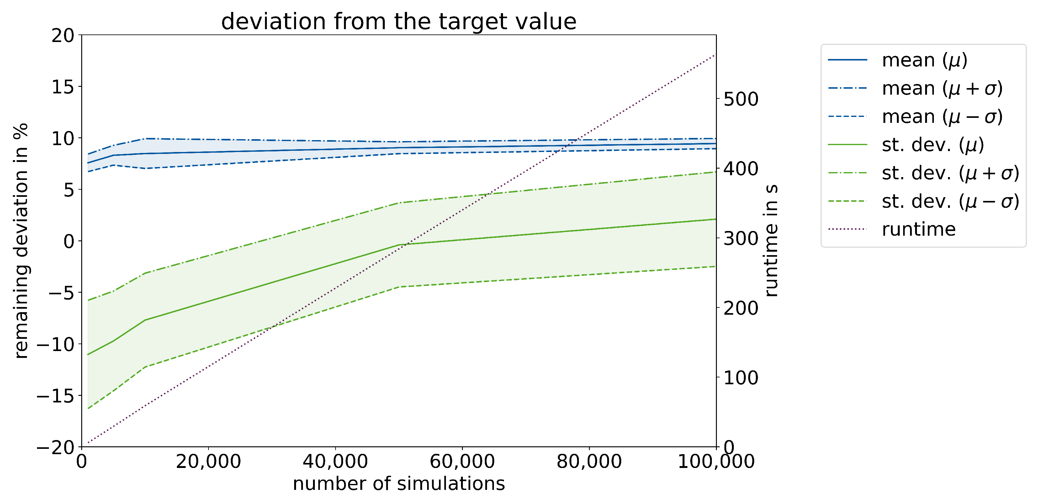
The results for a group of walls containing carbonation measurements of 5, 16, and 19 mm are given below. The first test was carried out to examine the influence of sample size (number of simulations) on the processing time and analyze the reproducibility of the process. To accomplish this, three runs were performed each for 1000, 5000, 10,000, 50,000, and 100,000 simulations with 4 bins. The results for carbonation are shown in Figure 3.
Although the deviation from the target value remained constant just below the termination criterion for the mean value, the remaining deviation after calibration decreased with the sample size for the standard deviation and amounts to approximately zero for 50,000 simulations. The standard deviation of the three runs did not seem to be significantly influenced by the number of simulations. To assess the runtime, a function was fitted over the bins and number of simulations, which is given in Equation (4). The number of simulations was nearly proportional to the overall runtime, with an exponent of 0.979. As there were other operations carried out in the script that amounted to part of the runtime, the deviation of this exponent from 1 is assumed to be due to overhead. Hereafter, the influence of N on the runtime is assumed to be proportional.
t ( b , N ) = 1.094 · 10 5 · b 4.718 · N 0.979
t : runtime in s b : number of bins N : number of simulations
To validate the performance of the approach by narrowing down the parameter boundaries iteratively, the tests were carried out with and without iterations for 50,000 simulations and 3 to 15 bins (see Figure 4). Figure 4a shows the deviation from the mean and although the approach with iterations undercuts the 10%-mark immediately for 3 bins, this is not the case without iterations for 15 bins. Looking at the standard deviation (Figure 4b), without iterations, 8 bins are required to fulfill the quality criterion.
The required runtime depending on the number of bins is given for the approach with and without iterations in Equations (5) and (6). Although the coefficient for the approach with iterations is higher by a power of two, the number of bins is more influential with a higher exponent for the approach without iterations.
t ( b , N ) = 3.780 · 10 5 · b 3.960 · N , with iteration
t ( b , N ) = 8.525 · 10 7 · b 4.956 · N , without iteration
t : runtime in s b : number of bins N : number of simulations
In order to achieve almost the same precision as the approach with iterations, it is assumed that the approach without iterations needs 15 bins instead of 3. This results in a runtime of 28,624 s (7.95 h) instead of 93 s, a 307-fold increase in runtime or a 99.7% reduction in processing time through the use of iterations.

3.2. Calibration of Chloride Model

Although the measurement of carbonation depths can easily be used as evidence for Bayesian inference, the evidence for chloride modeling is more complex as it has another dimension—the depth at which the chloride content was determined. When analyzing the chloride content from drill dust probes, only one value per depth step is obtained as the dust has gathered over a specific depth range. The number of steps and their depths should be fitted to the age and contamination of the considered component, as discussed in [52]. As the chloride model (see Equation (3)) is dependent on both time and depth, the evidence has to be handled accordingly. To depict the in situ situation as precisely as possible, the algorithm creates one node in the Bayesian network for each piece of evidence and sets a uniform distribution for x according to the depth step. In this example, the evidence will be derived from chloride content analyses carried out on three drill dust probes in steps of 15 mm.
The used evidence, as well as the calculation and its relative derivation for 4 bins and 50,000 simulations, is given in Table 4. It can be seen that the iteration process ended without reaching the termination criterion and, instead, reached a deadlock when trying to narrow down the parameter boundaries. The high deviations partly result from the low absolute values (0.022 wt%) and the challenge of determining the depth profiles. Figure 5a visualizes the deviations over the number of simulations with 4 bins and shows no significant influence of sample size on the results or reproducibility, except on the runtime. Figure 5b shows the calibrated model over the penetration depth versus the evidence.
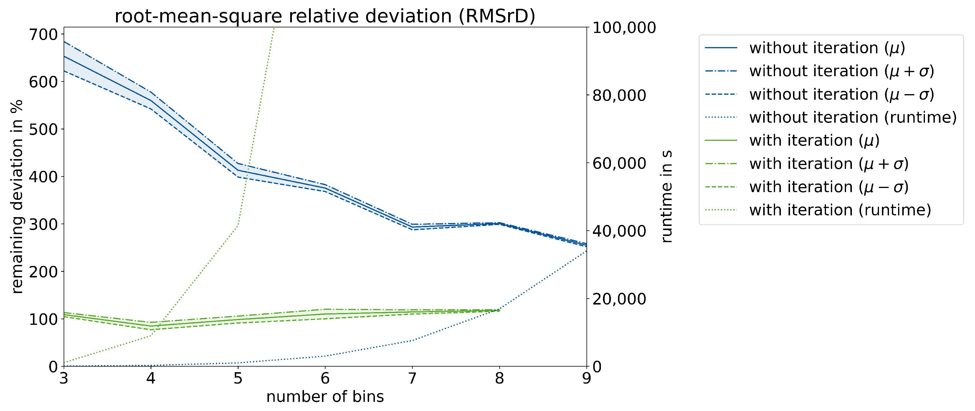
Although the remaining deviations in Table 4 and Figure 5 are higher than stipulated by the termination criterion, they have not yet been compared to the traditional method (without iterations). To perform a comparison that is comprehensible and combines the deviations over all depth steps, the root of the mean square relative deviations (RMSrD) was calculated. Figure 6 shows the RMSrD for 50,000 simulations and 3 to 9 bins with and without iterations. The approach with iterations was only carried out for up to 8 bins, as the processing time far exceeded the appropriate threshold.
The required runtime dependent on the number of bins is given in Equations (7) and (8) for the approach with and without iterations.
t ( b , N ) = 7.597 · 10 5 · b 6.077 · N , with iterations
t ( b , N ) = 1.416 · 10 6 · b 5.954 · N , without iterations
t : runtime in s b : number of bins N : number of simulations
Despite the longer processing time required by the iterative approach, due to its higher coefficient and a higher exponent for bins, it results in a significantly lower RMSrD than the non-iterative approach across all observed bins. Assuming a linear regression over the approach without iterations, 10.56 bins would be required to achieve the same RMSrD as the approach with iterations at 3 bins, leading to an 83-fold increase in the processing time for the same precision, or rather a 98.8% reduction in the processing time through the use of iterations. As the RMSrD curve without iterations would most probably not be linear but rather convergent, this can be considered strongly conservative.
The results of the iterative inference with 50,000 simulations and 4 bins for carbonation and chloride ingress are given in Table 5. For example, to achieve the carbonation depths according to the given evidence, the relative air humidity was calculated to be 43.75 ≤ 70.00 ± 9.81 ≤ 92.97%. For the evidenced chloride ingress, the interval size for the age exponent was narrowed down by 91.3% from 1 to 0.087.

3.3. Bayesian Inference in BIM

The BIM implementation of Bayesian inference allows for the selection of elements and the calibration of both deterioration models according to the available diagnosis data. As the implemented diagnosis data also contain measurements of concrete cover, the carbonation depth and chloride ingress can be compared with the (characteristic) concrete cover of the respective components. As a result, probabilistic durability assessments can be carried out directly in BIM using calibrated deterioration models and the actual concrete cover for each element. Figure 7 shows the probability of failure (depassivation) p f due to carbonation for several walls and columns ranging from 14.6% (green) to 61.0% (red). The red areas have a high risk of corrosion damage (initiation stage) from carbonation, whereas the green areas have a lower risk.
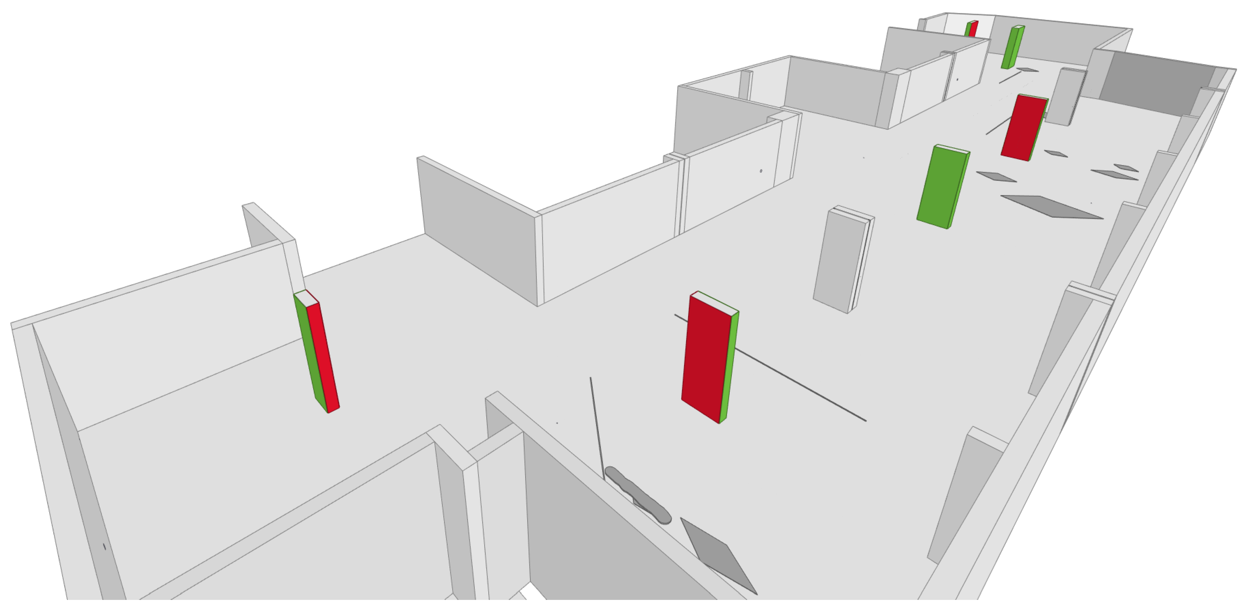
With both the diagnosis data and the calibrated deterioration modeling implemented, the BIM model can be used to assess the condition of the structure and inform decision making regarding the choice of repair measures. Principles and methods for the repair and prevention of damage to reinforced concrete structures are provided internationally in ISO 16311-3 [1], for Europe in EN 1504-9 [2], and for Germany in the technical standard “Maintenance of Concrete Structures” (TR IH) [3]. Although all these regulations allow more or less the same methods, the TR IH defines the specific conditions under which certain methods can or cannot be applied. These can be used to implement appropriate decision trees via Python/Dynamo and enable the automated assessments of methods. For example, method 7.1 is only applicable according to TR IH as long as the carbonation depth and depth of the critical chloride content are ≥ 10 mm from the concrete cover. This information is available as machine-readable data, allowing it to be applied to each individual surface. Figure 8 shows the applicability of method 7.1 (green = applicable, red = not applicable) assessed for each side of six columns viewed in BIMvision.
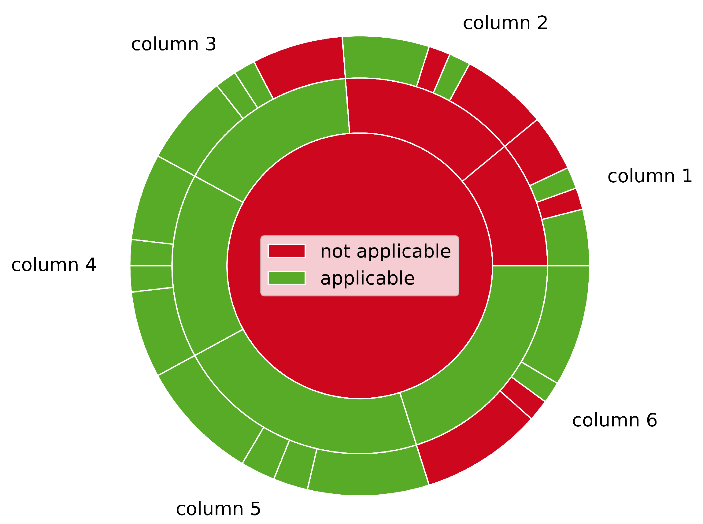
For practical reasons, it may not be feasible to assess each side of each column individually, as it may not be possible for the repair measures to be executed in such increments. This is why the assessment has been implemented to simultaneously consider each element side, each element, and the group of all elements as a whole. This can lead to different results, as shown in Figure 9. If all columns are considered at once, method 7.1 would not be applicable, as the characteristic concrete cover would be very low as a result of a very high standard deviation of the sample. Table 6 shows the proportion of elements and areas for which method 7.1 would be applicable. This analysis could also be performed for other methods and parameters such as the required removal of old concrete and the layer thickness of repair mortar.
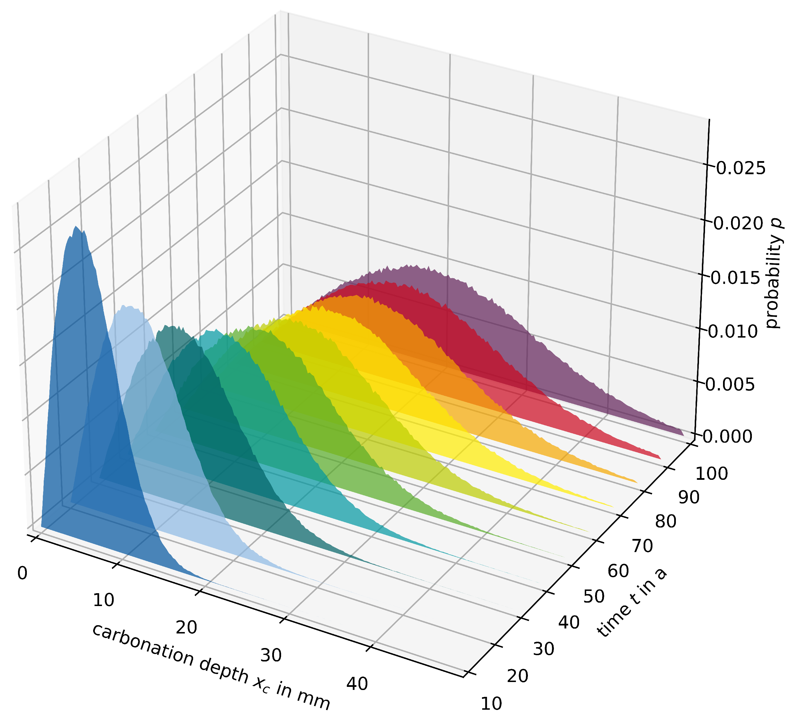
The integration of durability models into the BIM framework allows for the 3D assessment of dynamic component selections. In addition, the fourth dimension (time) can be taken into account, as the calculations are simultaneously carried out for the present, the near future (e.g., + 5 years), and the end of the life cycle. The corresponding numbers can be input at will, enabling 4D assessments of durability. Figure 10 shows the probability distribution of carbonation depth over time. It can be seen that both the mean values, as well as the 90%-quantiles, vary significantly depending on time.
Regarding Figure 2, the probability of failure is calculated in node B6 and the applicability of method 7.1 (and other methods for which decision trees were implemented) is assessed in node B7. The corresponding objects visualized in Figure 7 and Figure 8 were created in node C2. Figure 9 and Figure 10, as well as Table 6, were created with Python scripts that used the exported data from node C1 as input. These Python scripts could also be included in the Dynamo workflow, which might enable or assist report generation.

4. Discussion

4.1. Automated Bayesian Inference with Iteration

The automation of Bayesian inference enables iterative execution and thus new possibilities for novel approaches and analyses. Through the definition of termination criteria, acceptable limits for deviation, or rather a required precision of Bayesian inference, can be specified and, if possible, satisfied. In the presented research, ±10% deviation from the mean and, if more than two pieces of evidence are given, less than ±30% deviation from the standard deviation of carbonation depth(s), as well as ±20% deviation from the mean chloride content per-depth step, have proven to be productive. Nevertheless, these criteria can be adjusted arbitrarily and activated or deactivated at will. Other criteria could also be implemented, such as skewness, kurtosis, or virtually any other statistical aspect. In the given examples, the carbonation model was more likely to fulfill the criteria and achieve low remaining deviations a posteriori compared to the chloride model.
The sample size was identified as having a proportional influence on the processing time and almost no systematic influence on the deviations or reproducibility within the examined boundaries. The number of bins had a considerable effect on the runtime and the effectiveness of conventional Bayesian inference without iterations. Iterating the inference increased the required runtime per bin. However, significantly fewer bins were required to achieve proper results. This led to a 99.7% reduced runtime for carbonation and 98.8% reduced runtime for chloride ingress, achieving results similar to the process without iterations. Although reasonable results could be delivered with as few as 3 bins and 10,000 simulations, a combination of 4 bins and 50,000 simulations was deemed an adequate setting for reliable inference with iterations. With this setting, the calibration of the models took around 5 min for carbonation and 2.5 h for chloride ingress. All of the results shown are based on only one set of evidence for each model. It is expected that processing times and remaining deviations may vary significantly with other sets of evidence.
As mentioned above, the combination of carbonation and chloride ingress presents a challenge for reliable modeling and is currently being addressed by several researchers. A decent calibration of the individual models to the in situ conditions according to diagnosis data should, to a certain extent, automatically incorporate the interaction of these processes. Furthermore, any model parameters that are unknown or subject to discussion within the specialist community can be set to be updated. The proposed workflow is not only suited to compensating for this lack of information but also reducing it sustainably, as the calibrated parameters can be stored, shared, and assessed machine-readably in the context of a specific structure according to the BIM model. This may constitute one of the first steps toward big data in the durability assessment of structures, as it lays the foundation for gathering and evaluating machine-readable and thus communicable diagnosis data.

4.2. Predictive BIM as Decision Support Tool

By implementing automated Bayesian networks as calibration for deterioration models based on implemented diagnosis data, new functionality is achieved. This gives BIM predictive qualities and makes it a useful decision support tool for durability evaluation and maintenance planning. Adaptive selection and analysis of different components allow a systematic analysis of the underlying diagnosis data. Each evidence set and element selection can be assessed individually and automatically. In its current state, the workflow is accessible in a single piece of software (Revit) by importing the functionality of GeNIe via PySMILE through Dynamo into the BIM software. All the results are stored as IFC-compatible files in the model itself or the accompanying CSV files, ensuring full transparency and no information loss. As the calibration of the deterioration models is performed via Bayesian inference and not by opaque AI, the process is understandable. The algorithm saves the a priori and a posteriori networks for each iteration so that the progression of the calibration can be visualized and audited through both Python/PySMILE and GeNIe, which even offers a GUI.
The progress of carbonation and chloride ingress, as well as the probability of failure according to concrete cover, can be calculated for different elements and points in time, allowing four-dimensional durability assessments. Although the shown examples are constrained to the fib models for carbonation and chloride ingress, the models are fungible and could even be changed according to the situation in situ. For example, a model for cracked concrete could be selected if there are cracks on the selected element or parameters could be adjusted according to the deposited material, exposition, or inclination. In addition to this, a framework could be implemented to consider both the initiation and propagation stages, as demonstrated in [44,53].
Ultimately, the proposed workflow can be used to save resources, as it can assist in planning targeted and efficient repair measures. Damage could even be prevented if precise prognoses are available and practical to access. The model could also apply safety factors according to the sample size of diagnosis data, as proposed by [54], or recommend areas predestined for further measurements.

5. Conclusions and Outlook

In this paper, a novel approach to the calibration of deterioration models was demonstrated for carbonation and chloride ingress of reinforced concrete. The proposed workflow uses BIM enriched with machine-readable diagnosis data and Bayesian networks to automatically assess the present or future state of components individually or grouped depending on the selection. This achieves a predictive BIM model that can serve as a four-dimensional decision support tool. The following conclusions can be drawn from the presented research:
  • The automation of iterative Bayesian inference leads to significantly more efficient calibrations, as the processing times can be reduced by 99.7% for carbonation and 98.8% for chloride ingress compared to the conventional approach with similar precision.
  • The precision of the calibration process can be influenced by adjustable termination criteria, allowing individual configurations to be adjusted to project requirements.
  • As the deterioration models are calibrated according to the actual carbonation depths and chloride contents, the need for models for the combined effect of carbonation and chloride ingress, as well as alternative binders or concrete compositions, diminishes. The influence of these aspects is incorporated automatically, as well as the actual concrete cover per component.
  • The functionality of BIM can be extended significantly by combining BIM with Python according to wrappers. This way, the interoperability of several programs can be achieved while the user only operates one piece of software containing the combined functionality of all the implemented software.
  • By exporting the Bayesian networks and analysis results as CSV, TXT, and XDSL files, the workflow is transparent and traceable. The final results of the assessment are stored in automatically created BIM objects serving as data layers on the corresponding components. These objects are IFC compatible, allowing interoperability with other BIM software via enriched IFC files.
  • The combination of timely and spatially resolved, reliable deterioration models can be used to establish predictive BIM for maintenance and repair as a resource-efficient way of working.
As an outlook, predictive BIM could not only calibrate deterioration models and compare them to the given concrete cover but also take into account structural considerations such as macrocell corrosion. In cases where the front rebar layer is depassivated but the rear layer is still passive, which can be identified by BIM as shown above, accelerated macrocell corrosion can become relevant [55]. Besides refining models for chloride ingress, identifying the critical chloride content is of great relevance for durability, which is why the linking of structural engineering and materials science is proposed [56]. This could be achieved by incorporating diagnosis data and mathematical functionality into BIM.

Author Contributions

Conceptualization, H.M. and M.R.; Methodology, H.M. and M.R.; Software, H.M.; Validation, H.M.; Investigation, H.M.; Resources, M.R.; Data curation, H.M.; Writing—original draft, H.M.; Writing—review & editing, M.R.; Visualization, H.M; Supervision, M.R. All authors have read and agreed to the published version of the manuscript.

Funding

This research received no external funding.

Data Availability Statement

Not applicable.

Acknowledgments

The authors would like to acknowledge BayesFusion for providing the GeNIe-software and the SMILE-engine used in this research.

Conflicts of Interest

The authors declare that they have no conflict of interest.

Abbreviations

The following abbreviations are used in this manuscript:
AAMAlkali-Activated Materials
AIArtificial Intelligence
BIMBuilding Information Modeling
BMSBridge Monitoring System
CSVComma-Separated Values
DTDigital Twin
DTCDigital Twin Construction
GUIGraphical User Interface
IFCIndustry Foundation Classes
IoTInternet of Things
shBIMStructural Health BIM
SHMStructural Health Monitoring
TR IHTechnical Standard “Maintenance of Concrete Structures”
TXTtext file format
XDSLGeNIe’s native file format

References

  1. ISO 16311-3; Maintenance and Repair of Concrete Structures—Part 3: Design of Repairs and Prevention. Beuth: Berlin, Germany, 2014.
  2. DIN EN 1504-9; Produkte und Systeme für den Schutz und die Instandsetzung von Betontragwerken—Definitionen, Anforderungen, Qualitätsüberwachung und Beurteilung der Konformität—Teil 9: Allgemeine Grundsätze für die Anwendung von Produkten und Systemen. European Standard. Beuth: Berlin, Germany, 2008.
  3. Deutsches Institut für Bautechnik (DIBt). Technische Regel—Instandhaltung von Betonbauwerken (TR Instandhaltung); German Institut for Building Technology: Berlin, Germany, 2020. [Google Scholar]
  4. Driessen-Ohlenforst, C. SMART-DECK: Multifunctional carbon-reinforced concrete interlayer for bridges. Mater. Corros. 2020, 71, 786–796. [Google Scholar] [CrossRef] [Green Version]
  5. Herbrand, M.; Wenner, M.; Ullerich, C.; Rauert, T.; Zehetmaier, G.; Marx, S. Beurteilung der Bauwerkszuverlässigkeit durch Bauwerksmonitoring. Bautechnik 2021, 98, 93–104. [Google Scholar] [CrossRef]
  6. Sacks, R.; Girolami, M.; Brilakis, I. Building Information Modelling, Artificial Intelligence and Construction Tech. Dev. Built Environ. 2020, 4, 100011. [Google Scholar] [CrossRef]
  7. Yang, A.; Han, M.; Zeng, Q.; Sun, Y.; Liu, H. Adopting Building Information Modeling (BIM) for the Development of Smart Buildings: A Review of Enabling Applications and Challenges. Adv. Civ. Eng. 2021, 2021, 1–26. [Google Scholar] [CrossRef]
  8. Hamooni, M.; Maghrebi, M.; Majrouhi Sardroud, J.; Kim, S. Extending BIM Interoperability for Real-Time Concrete Formwork Process Monitoring. Appl. Sci. 2020, 10, 1085. [Google Scholar] [CrossRef] [Green Version]
  9. Byun, N.; Han, W.S.; Kwon, Y.W.; Kang, Y.J. Development of BIM-Based Bridge Maintenance System Considering Maintenance Data Schema and Information System. Sustainability 2021, 13, 4858. [Google Scholar] [CrossRef]
  10. Hartung, R.; Schönbach, R.; Liepe, D.; Klemt-Albert, K. Automatized Parametric Modeling to Enhance a data-based Maintenance Process for Infrastructure Buildings, 2020. In Proceedings of the 37th ISARC, Kitakyushu, Japan, 27–28 October 2020. [Google Scholar] [CrossRef]
  11. Boje, C.; Guerriero, A.; Kubicki, S.; Rezgui, Y. Towards a semantic Construction Digital Twin: Directions for future research. Autom. Constr. 2020, 114, 103179. [Google Scholar] [CrossRef]
  12. Sacks, R.; Brilakis, I.; Pikas, E.; Xie, H.S.; Girolami, M. Construction with digital twin information systems. Data-Centric Eng. 2020, 1, e14. [Google Scholar] [CrossRef]
  13. Camposano, J.C.; Smolander, K.; Ruippo, T. Seven Metaphors to Understand Digital Twins of Built Assets. IEEE Access 2021, 9, 27167–27181. [Google Scholar] [CrossRef]
  14. Kaewunruen, S.; AbdelHadi, M.; Kongpuang, M.; Pansuk, W.; Remennikov, A.M. Digital Twins for Managing Railway Bridge Maintenance, Resilience, and Climate Change Adaptation. Sensors 2022, 23, 252. [Google Scholar] [CrossRef]
  15. Nour El-Din, M.; Pereira, P.F.; Poças Martins, J.; Ramos, N.M.M. Digital Twins for Construction Assets Using BIM Standard Specifications. Buildings 2022, 12, 2155. [Google Scholar] [CrossRef]
  16. Uddin, M.N.; Wang, Q.; Wei, H.H.; Chi, H.L.; Ni, M. Building information modeling (BIM), System dynamics (SD), and Agent-based modeling (ABM): Towards an integrated approach. Ain Shams Eng. J. 2021, 12, 4261–4274. [Google Scholar] [CrossRef]
  17. Desogus, G.; Quaquero, E.; Rubiu, G.; Gatto, G.; Perra, C. BIM and IoT Sensors Integration: A Framework for Consumption and Indoor Conditions Data Monitoring of Existing Buildings. Sustainability 2021, 13, 4496. [Google Scholar] [CrossRef]
  18. Gerbino, S.; Cieri, L.; Rainieri, C.; Fabbrocino, G. On BIM Interoperability via the IFC Standard: An Assessment from the Structural Engineering and Design Viewpoint. Appl. Sci. 2021, 11, 11430. [Google Scholar] [CrossRef]
  19. Panah, R.S.; Kioumarsi, M. Application of Building Information Modelling (BIM) in the Health Monitoring and Maintenance Process: A Systematic Review. Sensors 2021, 21, 837. [Google Scholar] [CrossRef]
  20. Morgenstern, H.; Raupach, M. BIM-centred building diagnoses as a decision support tool for maintenance and repair. e-J. Nondestruct. Test. 2022, 27, 9. [Google Scholar] [CrossRef]
  21. Morgenstern, H.; Raupach, M. Quantified point clouds and enriched BIM-Models for digitalised maintenance planning. MATEC Web Conf. 2022, 364, 05001. [Google Scholar] [CrossRef]
  22. Morgenstern, H.; Raupach, M. A Novel Approach for Maintenance and Repair of Reinforced Concrete Using Building Information Modeling with Integrated Machine-Readable Diagnosis Data. Constr. Mater. 2022, 2, 314–327. [Google Scholar] [CrossRef]
  23. Collao, J.; Lozano-Galant, F.; Lozano-Galant, J.A.; Turmo, J. BIM Visual Programming Tools Applications in Infrastructure Projects: A State-of-the-Art Review. Appl. Sci. 2021, 11, 8343. [Google Scholar] [CrossRef]
  24. Possan, E.; Andrade, J.J.O.; Dal Molin, D.C.C.; Ribeiro, J.L.D. Model to Estimate Concrete Carbonation Depth and Service Life Prediction. In Hygrothermal Behaviour and Building Pathologies; Building Pathology and Rehabilitation; Book Section Chapter 4; Springer: Cham, Switzerland, 2021; pp. 67–97. [Google Scholar] [CrossRef]
  25. Xia, J.; Shen, J.; Li, T.; Jin, W.L. Corrosion prediction models for steel bars in chloride-contaminated concrete: A review. Mag. Concr. Res. 2022, 74, 123–142. [Google Scholar] [CrossRef]
  26. Al-Ameeri, A.S.; Rafiq, M.I.; Tsioulou, O. Combined impact of carbonation and crack width on the Chloride Penetration and Corrosion Resistance of Concrete Structures. Cem. Concr. Compos. 2021, 115, 103819. [Google Scholar] [CrossRef]
  27. Zhu, X.; Zi, G.; Sun, L.; You, I. A simplified probabilistic model for the combined action of carbonation and chloride ingress. Mag. Concr. Res. 2019, 71, 327–340. [Google Scholar] [CrossRef]
  28. Shen, X.H.; Jiang, W.Q.; Hou, D.; Hu, Z.; Yang, J.; Liu, Q.F. Numerical study of carbonation and its effect on chloride binding in concrete. Cem. Concr. Compos. 2019, 104, 103402. [Google Scholar] [CrossRef]
  29. Zhu, X.; Zi, G.; Lee, W.; Kim, S.; Kong, J. Probabilistic analysis of reinforcement corrosion due to the combined action of carbonation and chloride ingress in concrete. Constr. Build. Mater. 2016, 124, 667–680. [Google Scholar] [CrossRef]
  30. Li, K.; Zhao, F.; Zhang, Y. Influence of carbonation on the chloride ingress into concrete: Theoretical analysis and application to durability design. Cem. Concr. Res. 2019, 123, 105788. [Google Scholar] [CrossRef]
  31. Bai, Y.; Wang, Y.; Xi, Y. Modeling the effect of temperature gradient on moisture and ionic transport in concrete. Cem. Concr. Compos. 2020, 106, 103454. [Google Scholar] [CrossRef]
  32. Pacheco, J. Incorporating Cracks in Chloride Ingress Modeling and Service Life Predictions. ACI Mater. J. 2019, 116, 113–118. [Google Scholar] [CrossRef]
  33. Mundra, S.; Prentice, D.P.; Bernal, S.A.; Provis, J.L. Modelling chloride transport in alkali-activated slags. Cem. Concr. Res. 2020, 130, 106011. [Google Scholar] [CrossRef]
  34. Mangat, P.S.; Ojedokun, O.O.; Lambert, P. Chloride-initiated corrosion in alkali activated reinforced concrete. Cem. Concr. Compos. 2021, 115, 103823. [Google Scholar] [CrossRef]
  35. Beushausen, H.; Torrent, R.; Alexander, M.G. Performance-based approaches for concrete durability: State of the art and future research needs. Cem. Concr. Res. 2019, 119, 11–20. [Google Scholar] [CrossRef]
  36. Adadi, A.; Berrada, M. Peeking Inside the Black-Box: A Survey on Explainable Artificial Intelligence (XAI). IEEE Access 2018, 6, 52138–52160. [Google Scholar] [CrossRef]
  37. Fink, O.; Wang, Q.; Svensén, M.; Dersin, P.; Lee, W.J.; Ducoffe, M. Potential, challenges and future directions for deep learning in prognostics and health management applications. Eng. Appl. Artif. Intell. 2020, 92, 103678. [Google Scholar] [CrossRef]
  38. Sun, L.; Shang, Z.; Xia, Y.; Bhowmick, S.; Nagarajaiah, S. Review of Bridge Structural Health Monitoring Aided by Big Data and Artificial Intelligence: From Condition Assessment to Damage Detection. J. Struct. Eng. 2020, 146, 22. [Google Scholar] [CrossRef]
  39. Ghahramani, Z. Probabilistic machine learning and artificial intelligence. Nature 2015, 521, 452–459. [Google Scholar] [CrossRef] [PubMed]
  40. Pradhan, A.; Dutta, N.C.; Le, H.Q.; Biondi, B.; Mukerji, T. Approximate Bayesian inference of seismic velocity and pore-pressure uncertainty with basin modeling, rock physics, and imaging constraints. Geophysics 2020, 85, ID19–ID34. [Google Scholar] [CrossRef]
  41. Cui, Y.; Zhu, Z.; Zhao, X.; Li, Z.; Qin, P. Bayesian Calibration for Office-Building Heating and Cooling Energy Prediction Model. Buildings 2022, 12, 1052. [Google Scholar] [CrossRef]
  42. Ashtari, M.A.; Ansari, R.; Hassannayebi, E.; Jeong, J. Cost Overrun Risk Assessment and Prediction in Construction Projects: A Bayesian Network Classifier Approach. Buildings 2022, 12, 1660. [Google Scholar] [CrossRef]
  43. Jung, H.; Im, S.B.; An, Y.K. Probability-Based Concrete Carbonation Prediction Using On-Site Data. Appl. Sci. 2020, 10, 4330. [Google Scholar] [CrossRef]
  44. Hackl, J.; Kohler, J. Reliability assessment of deteriorating reinforced concrete structures by representing the coupled effect of corrosion initiation and progression by Bayesian networks. Struct. Saf. 2016, 62, 12–23. [Google Scholar] [CrossRef]
  45. Straub, D.; Papaioannou, I. Bayesian Updating with Structural Reliability Methods. J. Eng. Mech. 2015, 141, 13. [Google Scholar] [CrossRef] [Green Version]
  46. Cai, B.; Kong, X.; Liu, Y.; Lin, J.; Yuan, X.; Xu, H.; Ji, R. Application of Bayesian Networks in Reliability Evaluation. IEEE Trans. Ind. Inform. 2019, 15, 2146–2157. [Google Scholar] [CrossRef] [Green Version]
  47. Straub, D.; Papaioannou, I.; Betz, W. Bayesian analysis of rare events. J. Comput. Phys. 2016, 314, 538–556. [Google Scholar] [CrossRef]
  48. Büchter, T.; Eichler, A.; Steib, N.; Binder, K.; Böcherer-Linder, K.; Krauss, S.; Vogel, M. How to Train Novices in Bayesian Reasoning. Mathematics 2022, 10, 1558. [Google Scholar] [CrossRef]
  49. Schneider, R.; Fischer, J.; Bügler, M.; Nowak, M.; Thöns, S.; Borrmann, A.; Straub, D. Assessing and updating the reliability of concrete bridges subjected to spatial deterioration - principles and software implementation. Struct. Concr. 2015, 16, 356–365. [Google Scholar] [CrossRef]
  50. Fédération Internationale du Béton (fib). Model Code for Service Life Design; fib Bulletins; International Federation for Structural Concrete: Lausanne, Switzerland, 2006; Volume 34. [Google Scholar] [CrossRef]
  51. Grantham, M.G.; Gulikers, J.; Mircea, C. Predicting residual service life of concrete infrastructure: A considerably controversial subject. MATEC Web Conf. 2019, 289, 08002. [Google Scholar] [CrossRef]
  52. Kosalla, M.; Raupach, M. Diagnosis of concrete structures: The influence of sampling parameters on the accuracy of chloride profiles. Mater. Struct. 2018, 51, 75. [Google Scholar] [CrossRef]
  53. Bichara, L.; Saad, G.; Slika, W. Probabilistic identification of the effects of corrosion propagation on reinforced concrete structures via deflection and crack width measurements. Mater. Struct. 2019, 52, 89. [Google Scholar] [CrossRef]
  54. Marx, S.; Grünberg, J.; Schacht, G. Methoden zur Bewertung experimenteller Ergebnisse bei kleinem Stichprobenumfang. Betonund Stahlbetonbau 2018, 114, 2–13. [Google Scholar] [CrossRef] [Green Version]
  55. Chalhoub, C.; François, R.; Garcia, D.; Laurens, S.; Carcasses, M. Macrocell corrosion of steel in concrete: Characterization of anodic behavior in relation to the chloride content. Mater. Corros. 2020, 71, 1424–1441. [Google Scholar] [CrossRef]
  56. Angst, U.M. Predicting the time to corrosion initiation in reinforced concrete structures exposed to chlorides. Cem. Concr. Res. 2019, 115, 559–567. [Google Scholar] [CrossRef]
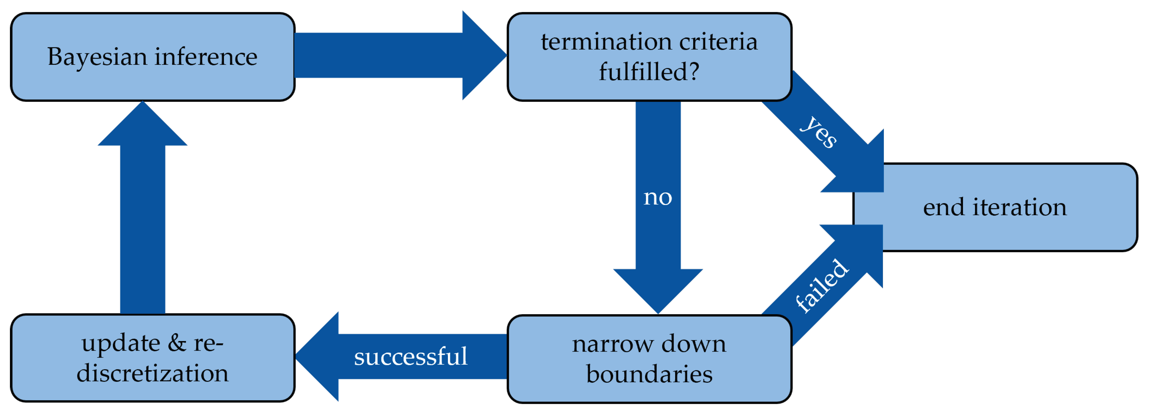
Figure 1. Flowchart of the iterative inference process.
Civileng 04 00012 g001
Figure 2. Compressed Dynamo script for implementing Bayesian inference and reliability assessment in Revit divided into (A) input, (B) analysis, and (C) output.
Civileng 04 00012 g002
Figure 3. Deviation from target value (mean and standard deviation) and required runtime over number of simulations for carbonation.
Civileng 04 00012 g003
Figure 4. Deviation from target value ((a) mean and (b) standard deviation) and required runtime over number of bins for carbonation.
Civileng 04 00012 g004
Figure 5. (a) Deviation from target value of required runtime over the number of simulations for chloride ingress. (b) Modeled mean chloride content over penetration depths versus evidence.
Civileng 04 00012 g005
Figure 6. Root of the mean square relative deviations (RMSrD) and required runtime over the number of bins for chloride ingress.
Civileng 04 00012 g006
Figure 7. (a) Visualization of probability of failure due to carbonation p f in BIMvision. (b) Legend/color code of p f .
Civileng 04 00012 g007
Figure 8. Applicability of method 7.1 assessed for each side of six columns viewed in BIMvision.
Civileng 04 00012 g008
Figure 9. Applicability of method 7.1 assessed for the group of six columns (innermost circle), each column individually (middle circle), and each side of each column (outer circle).
Civileng 04 00012 g009
Figure 10. Probability distribution of the carbonation depth over the time.
Civileng 04 00012 g010
Table 1. Parameters to be calibrated and their boundaries for carbonation.
ParameterLower BoundUpper BoundUnit
R H i s 0100%
k t 05
R A C C , 0 1 020,000(mm 2 /a)/(kg/m 3 )
ε t 11000(mm 2 /a)/(kg/m 3 )
C S , a t m 00.01977kg/m 3
Table 2. Parameters to be calibrated and their boundaries for chloride ingress.
ParameterLower BoundUpper BoundUnit
C l Δ x 05wt%
Δ x 050mm
b e 010,000K
T i s 233.15333.15K
D R C M , 0 0200mm 2 /a
a01
Table 3. Software used for BIM-based Bayesian inference.
SoftwareVersionDeveloperLocationFunction
Revit22.0.2.392AutodeskSan Rafael, USABIM author software
BIMvision2.25.2DatacompCracow, PolandBIM viewer
Dynamo2.10.1.4002AutodeskSan Rafael, USA(Visual) Programming in BIM
Python3.8.3Python Software FoundationWilmington, USAProgramming language
GeNIe4.0.2304.0BayesFusionPittsburgh, USABayesian network software
PySMILE2.0.8BayesFusionPittsburgh, USAPython wrapper for GeNIe
Table 4. Evidence, calculation, and relative deviation over three depth steps for 4 bins and 50,000 simulations.
DepthEvidenceCalculationRelative Deviation
in mmin wt%in wt%in %
0–151.9151.463−23.60
15–300.2940.40437.37
30–450.0220.053140.0
Table 5. Calibrated parameters and their boundaries posterior to the iterative inference for carbonation and chloride ingress.
ParameterLower BoundUpper BoundMeanStandard DeviationUnit
R H i s 43.7592.9770.009.81%
k t 0.3522.8131.5250.543
R A C C , 0 1 1230984450301851(mm 2 /a)/(kg/m 3 )
ε t 1562.9330.1143.3(mm 2 /a)/(kg/m 3 )
C S , a t m 00.003520.000450.00027kg/m 3
C l Δ x 1.4211.9141.6450.100wt%
Δ x 3.4348.7595.7601.156mm
b e 250044633337440K
T i s 265.8278.7272.82.8K
D R C M , 0 47.5989.6767.828.32mm 2 /a
a0.3740.4610.4180.019
Table 6. Applicability of method 7.1 assessed for the group of six columns, each column individually, each side of each column, and the corresponding area.
SelectionApplicative ElementsApplicative Area
-#%m 2 %
group0 of 10.00.0 of 44.90.0
component4 of 666.733.1 of 44.973.8
sides17 of 2470.831.6 of 44.970.4
Disclaimer/Publisher’s Note: The statements, opinions and data contained in all publications are solely those of the individual author(s) and contributor(s) and not of MDPI and/or the editor(s). MDPI and/or the editor(s) disclaim responsibility for any injury to people or property resulting from any ideas, methods, instructions or products referred to in the content.