
Site-Specific Response Spectra and Accelerograms on Bedrock and Soil Surface


Abstract
:1. Introduction
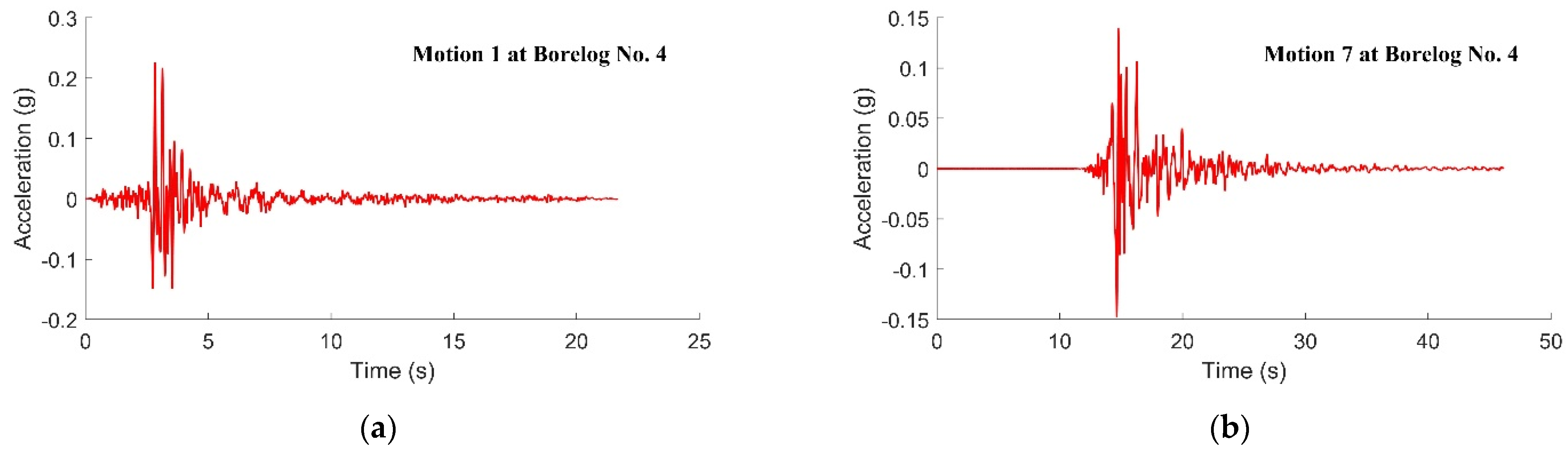
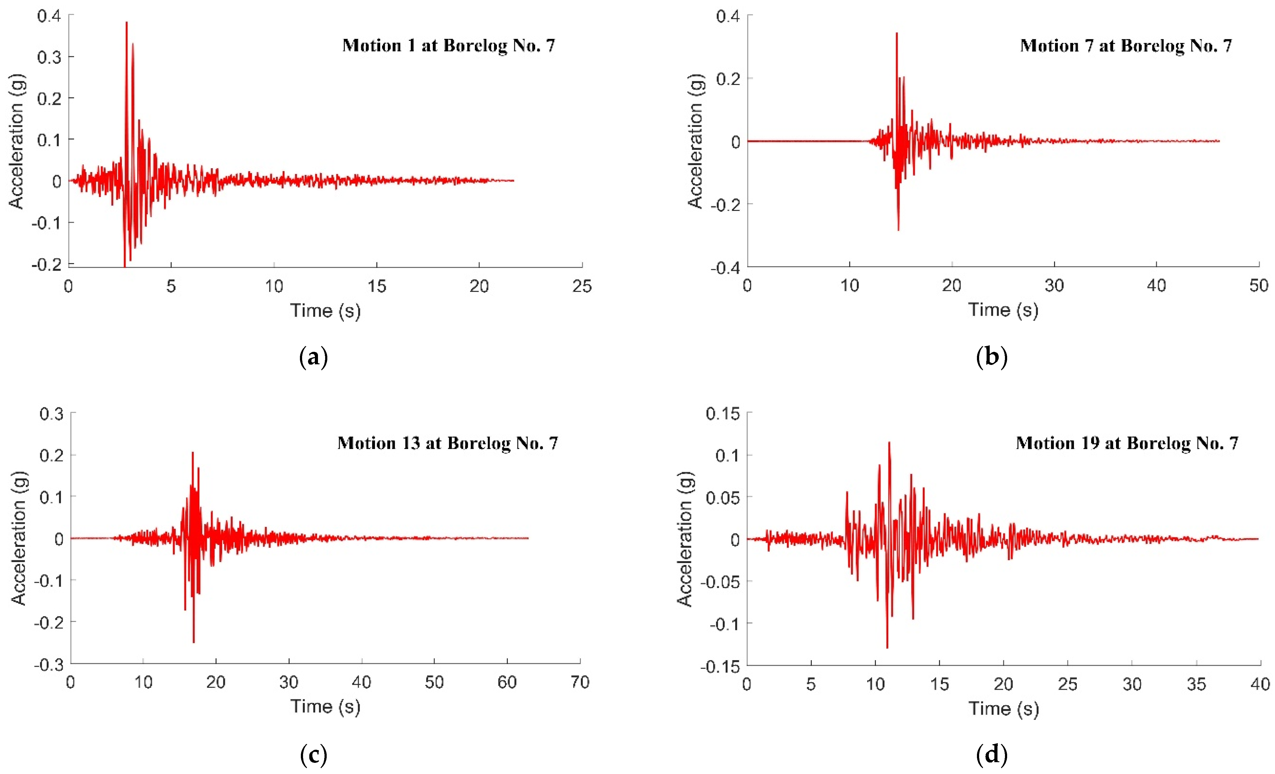
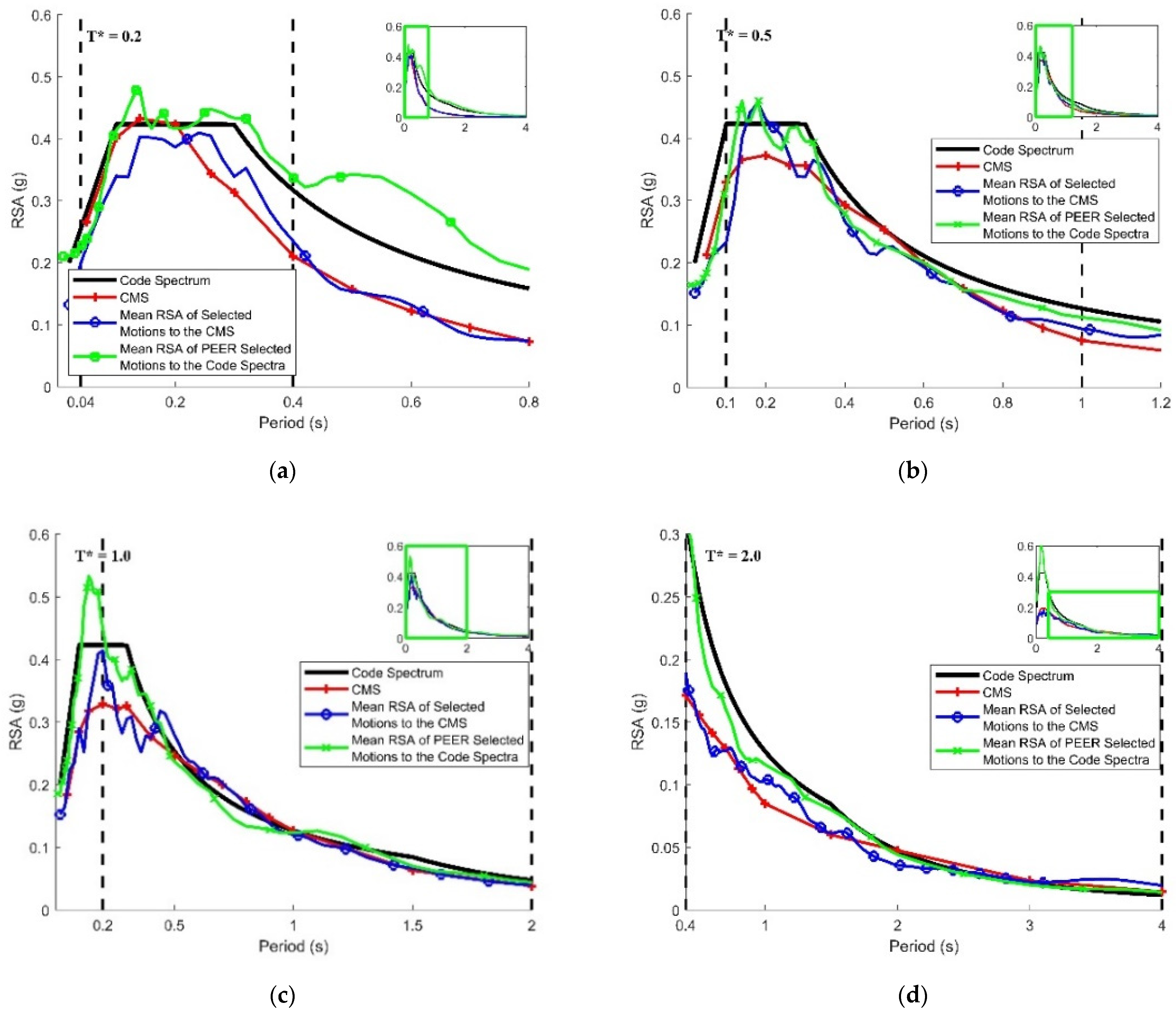
2. Accelerograms on Rock Sites: Datasets, Selection and Scaling
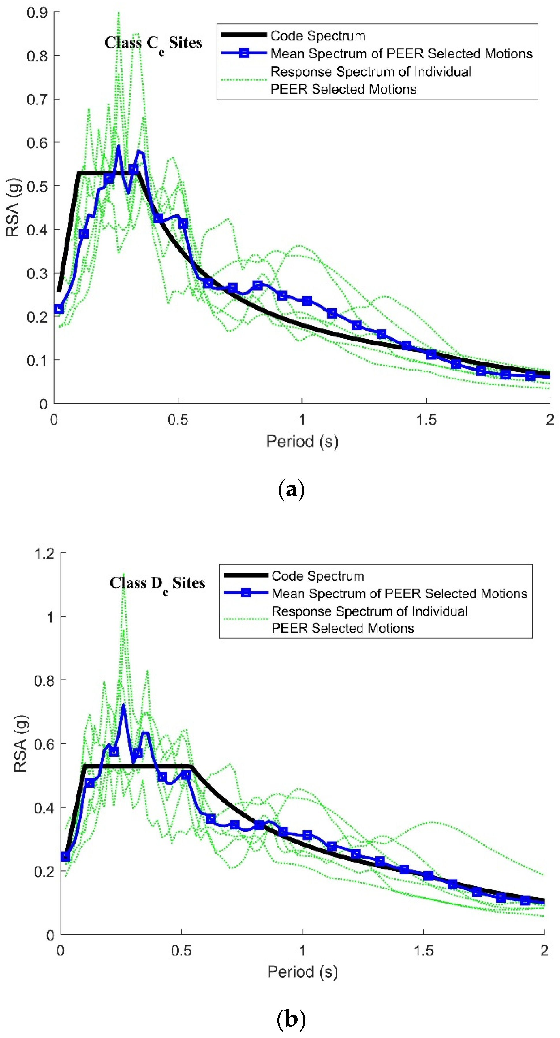
3. Event-Specific Spectra and Conditional Mean Spectra
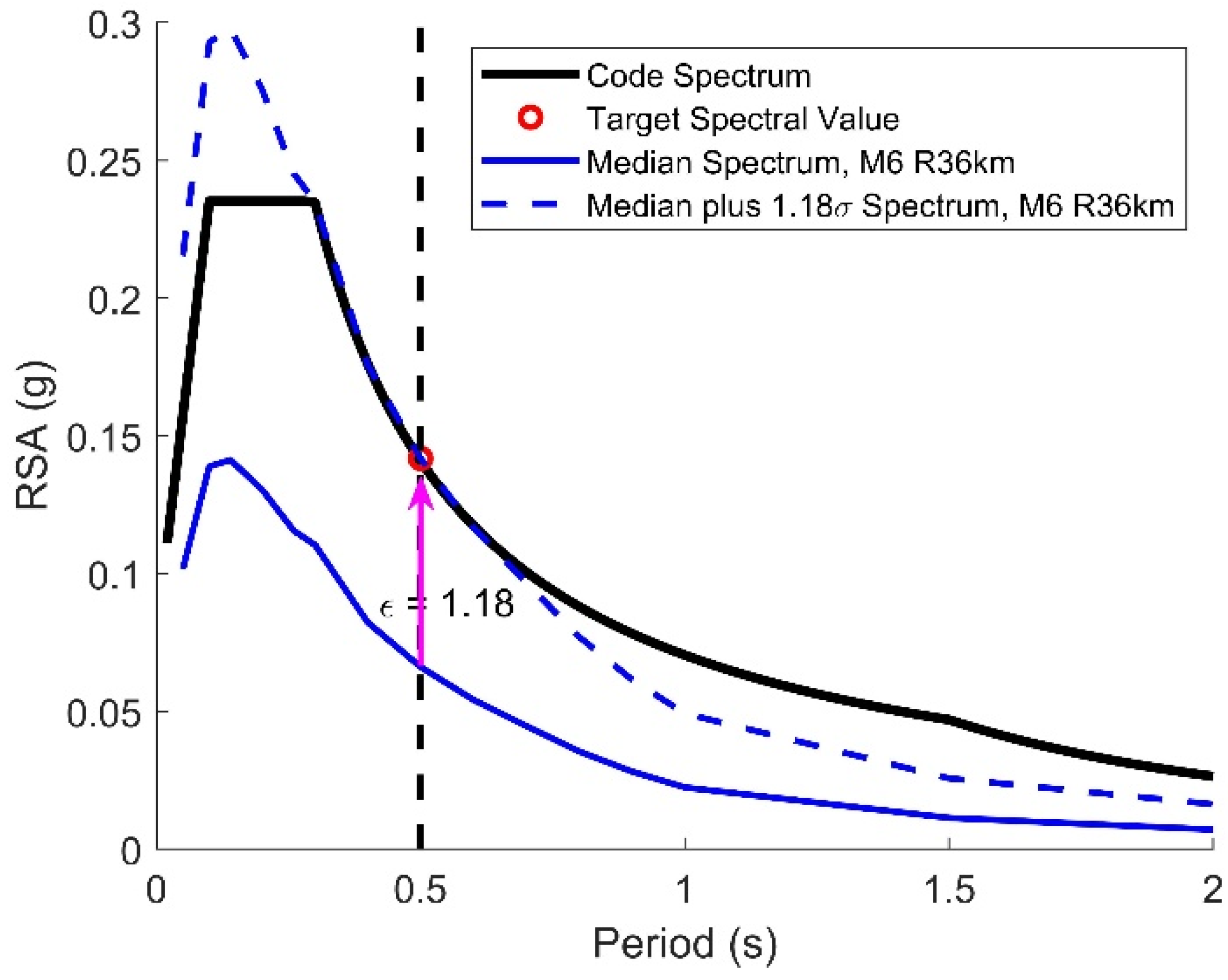
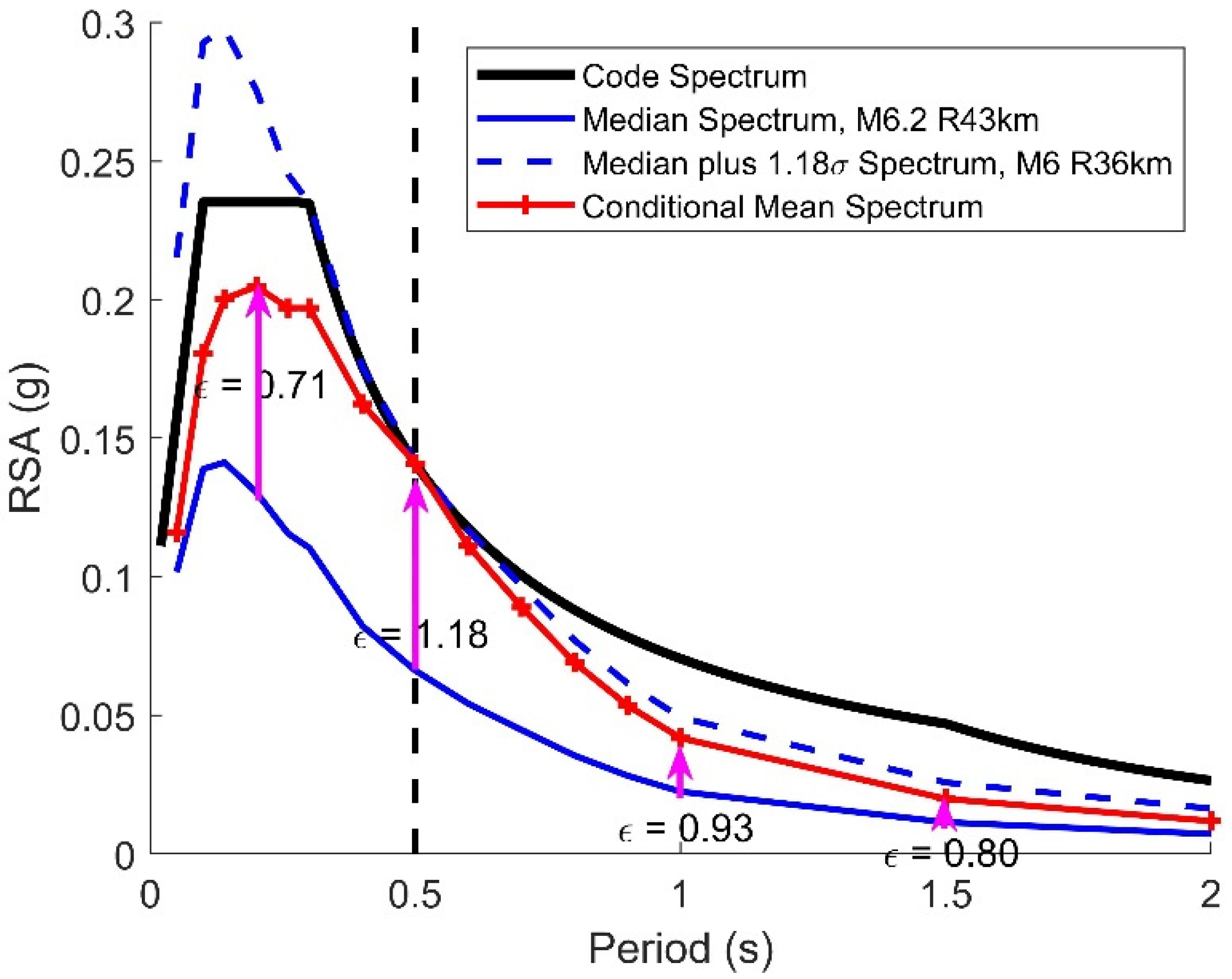
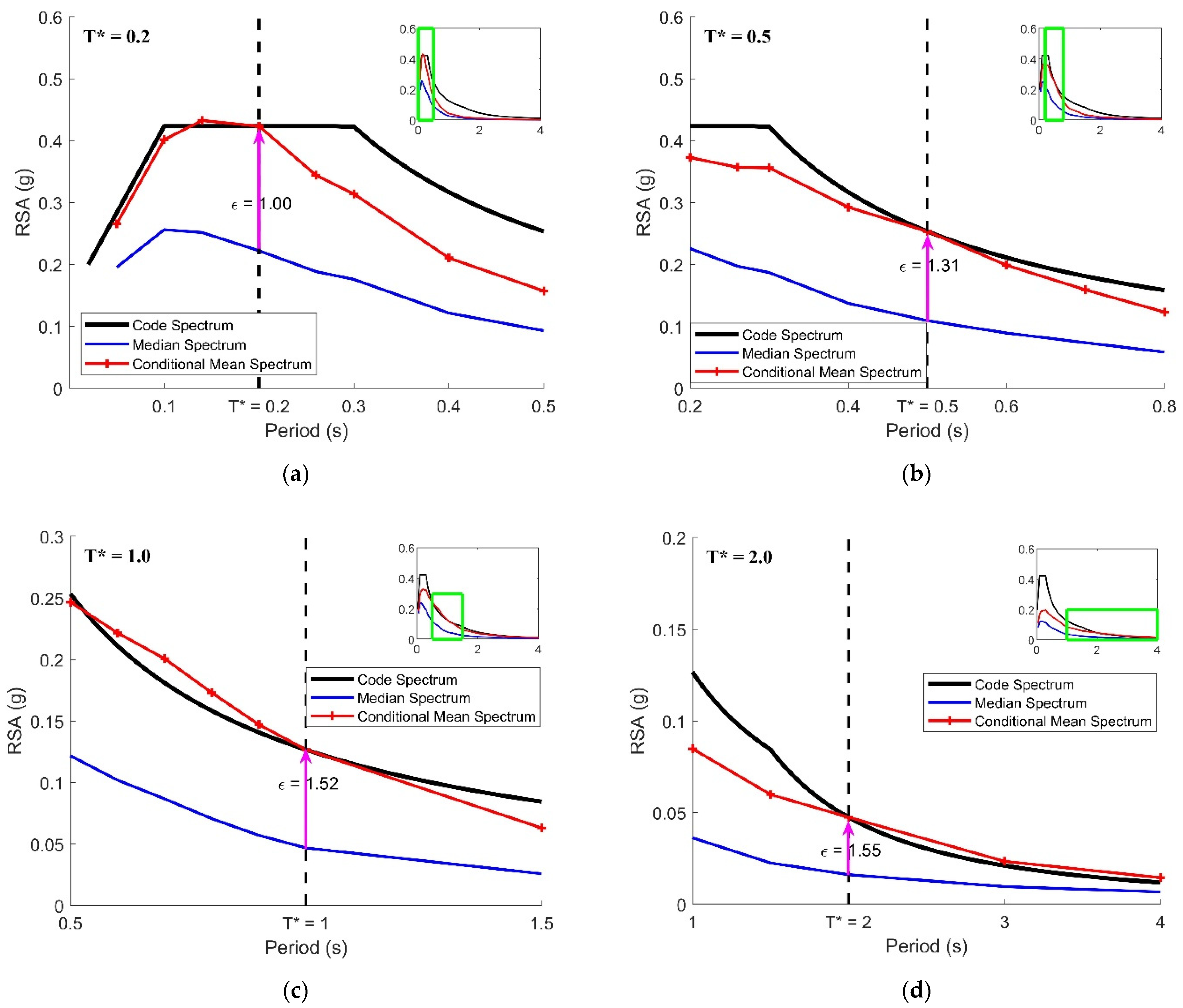
- Step 1—Identify the reference period () where matching with the code spectrum is to occur;
- Step 2—Identify the response spectral value of the code spectrum at or ;
- Step 3—Determine the earthquake scenario as expressed in terms of the M-R combination through hazard deaggregation analysis [19], the corresponding estimated median spectral values , and the standard deviation for the considered earthquake scenario;
- Step 4—Calculate the value of epsilon, , to achieve the response spectral value of the CMS at the reference period (which is defined as the sum of the median and the product of two factors: (i) standard deviation and (ii) epsilon, ε, matching the value of , as stipulated by the code;
- Step 5—Construct the CMS for a range of periods based on taking the sum of the median and product of three factors: (i) standard deviation , (ii) epsilon, ε, as determined in Step 4, and (iii) period-dependent correlation coefficient .
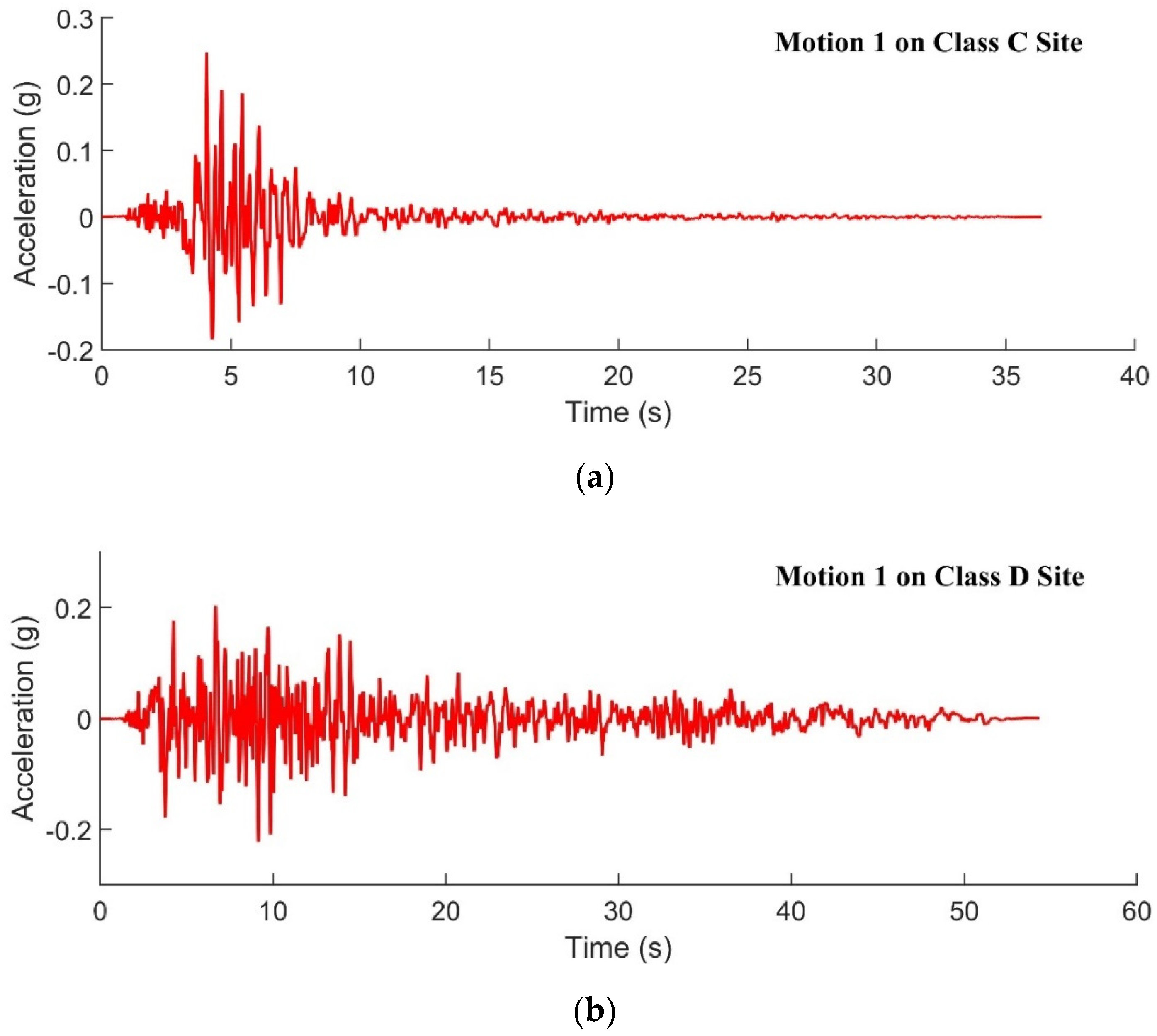
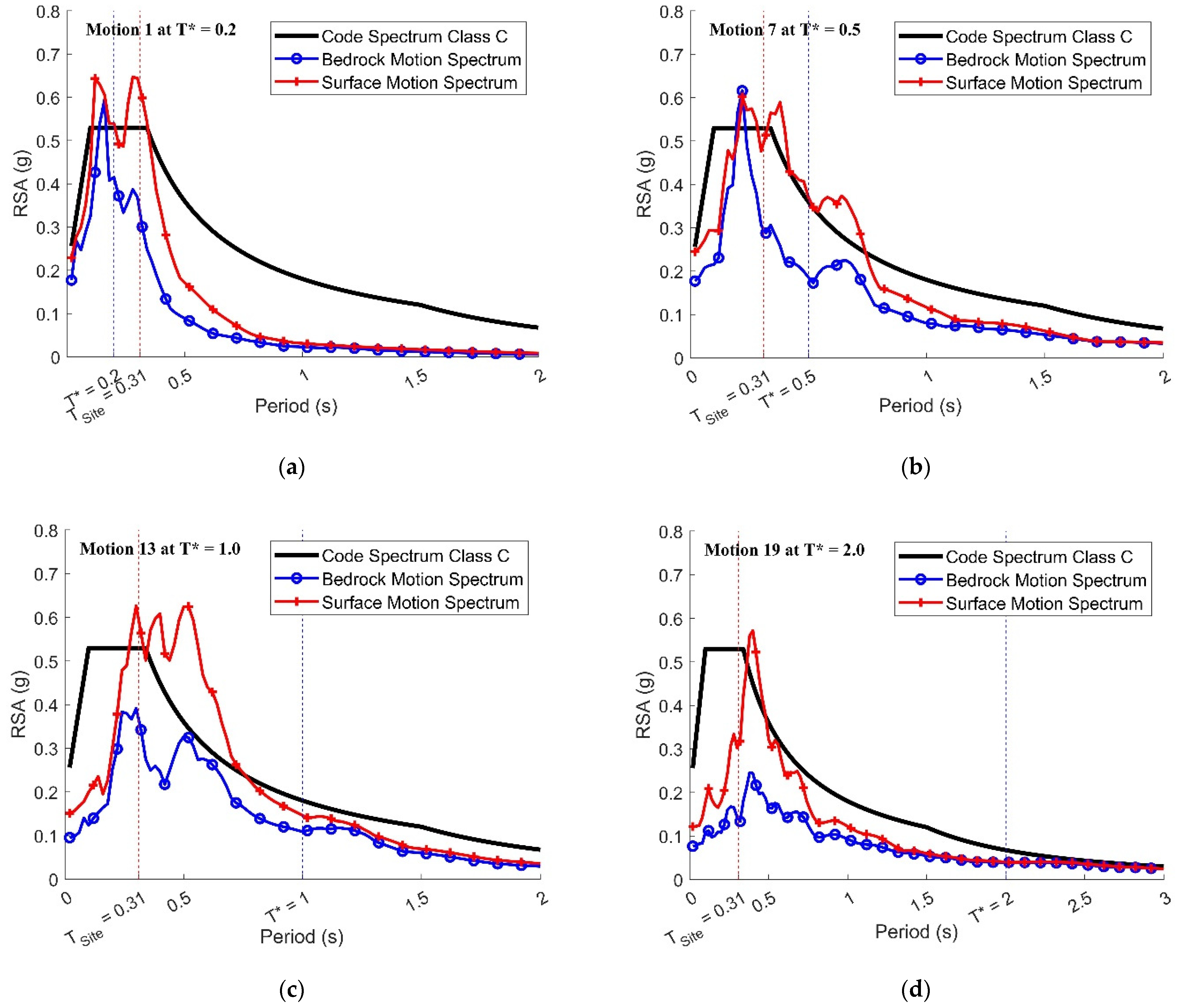
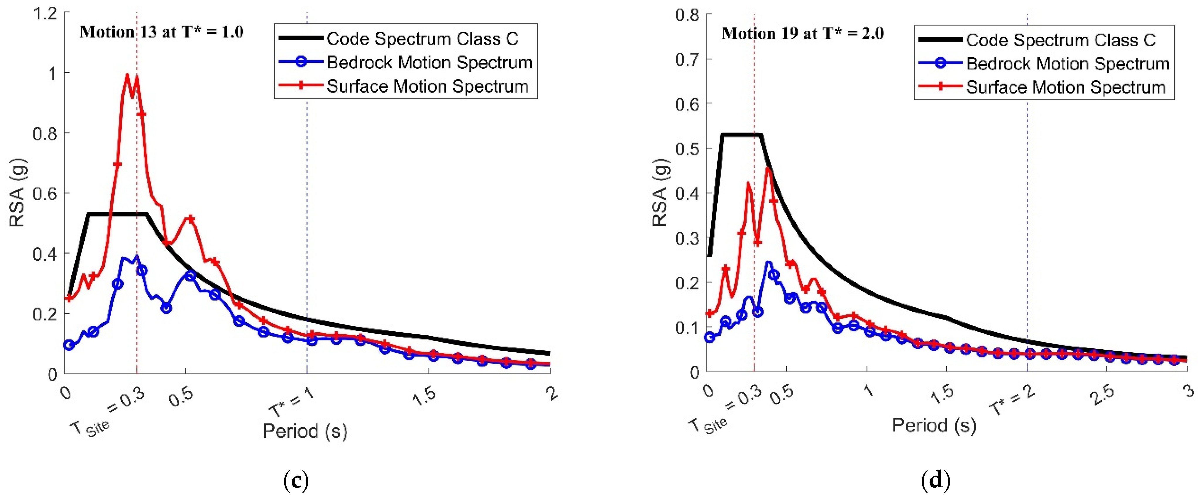
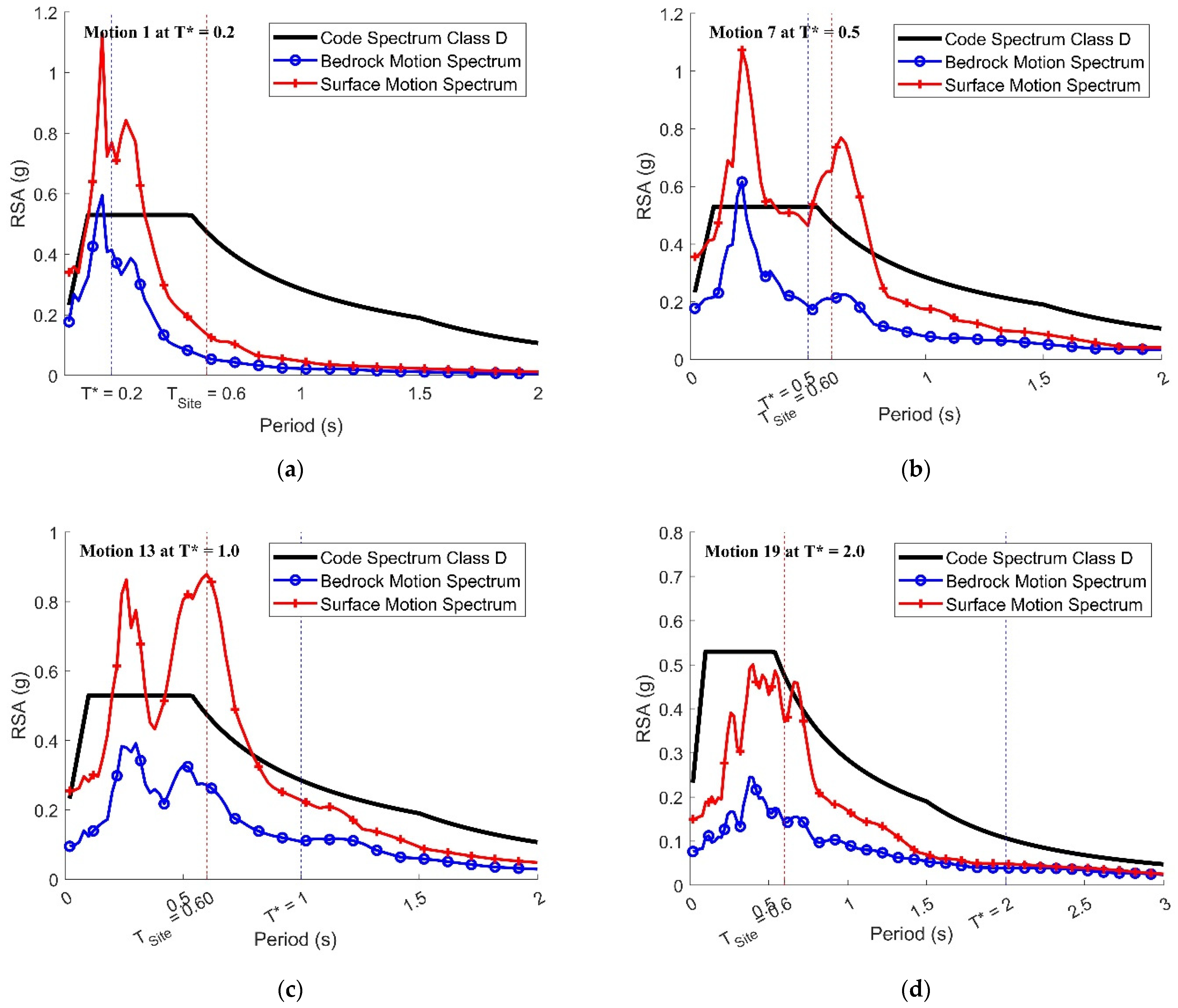
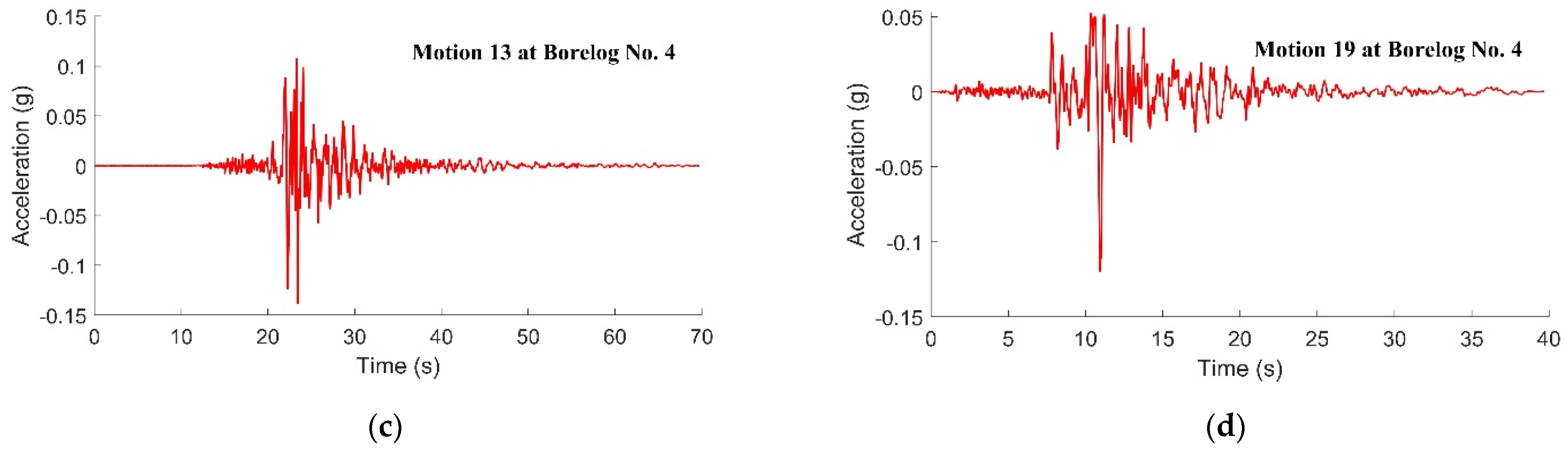
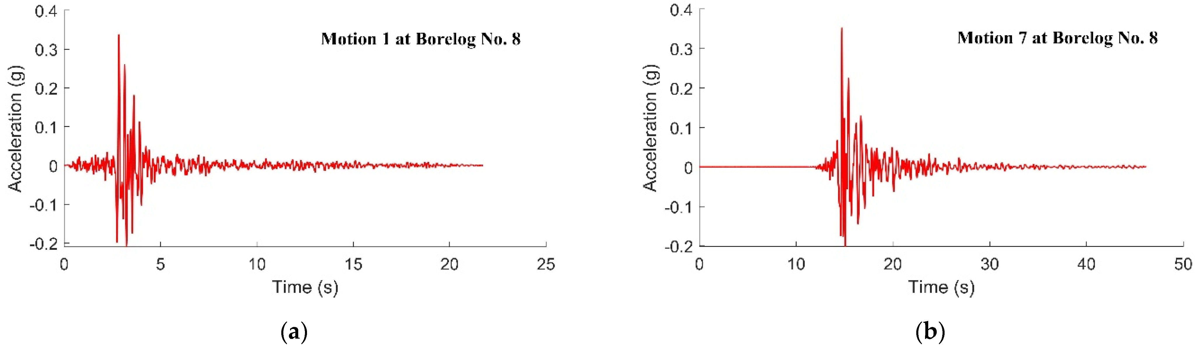
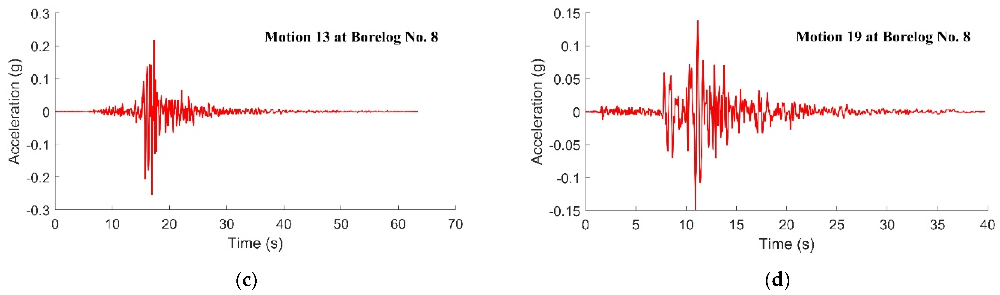
4. Accelerograms and Response Spectra on the Soil Surface
5. Conclusions
Author Contributions
Funding
Data Availability Statement
Acknowledgments
Conflicts of Interest
References
- Hanks, T.C.; McGuire, R.K. The character of high-frequency strong ground motion. Bull. Seismol. Soc. Am. 1981, 71, 2071–2095. [Google Scholar] [CrossRef]
- Boore, D.M. Stochastic simulation of high-frequency ground motions based on seismological models of the radiated spectra. Bull. Seismol. Soc. Am. 1983, 73, 1865–1894. [Google Scholar]
- Atkinson, G.M.; Boore, D.M. Ground-motion relations for eastern North America. Bull. Seismol. Soc. Am. 1995, 85, 17–30. [Google Scholar] [CrossRef]
- Atkinson, G.M.; Boore, D.M. Evaluation of models for earthquake source spectra in eastern North America. Bull. Seismol. Soc. Am. 1998, 88, 917–934. [Google Scholar] [CrossRef]
- Atkinson, G.M.; Silva, W. Stochastic modeling of California ground motions. Bull. Seismol. Soc. Am. 2000, 90, 255–274. [Google Scholar] [CrossRef]
- Atkinson, G.M.; Boore, D.M. Earthquake ground-motion prediction equations for eastern North America. Bull. Seismol. Soc. Am. 2006, 96, 2181–2205. [Google Scholar] [CrossRef] [Green Version]
- Boore, D.M. Point-Source Stochastic-Method Simulations of Ground Motions for the PEER NGA-East Project; Pacific Earthquake Engineering Research Center (PEER): Berkeley, CA, USA, 2015; pp. 11–49. [Google Scholar]
- Tang, Y.; Lam, N.T.; Tsang, H.-H.; Lumantarna, E. An adaptive ground motion prediction equation for use in low-to-moderate seismicity regions. J. Earthq. Eng. 2022, 26, 2567–2598. [Google Scholar] [CrossRef]
- Boore, D.M.; Joyner, W.B. Site amplifications for generic rock sites. Bull. Seismol. Soc. Am. 1997, 87, 327–341. [Google Scholar] [CrossRef]
- Silva, W.; Darragh, R.; Gregor, N.; Martin, G.; Abrahamson, N.; Kircher, C. Reassessment of Site Coefficients and Near-Fault Factors for Building Code Provisions; US Department of the Interior, US Geological Survey: Reston, VA, USA, 1999. [Google Scholar]
- Chandler, A.; Lam, N.; Tsang, H. Shear wave velocity modelling in crustal rock for seismic hazard analysis. Soil Dyn. Earthq. Eng. 2005, 25, 167–185. [Google Scholar] [CrossRef]
- Chandler, A.; Lam, N.; Tsang, H. Near-surface attenuation modelling based on rock shear-wave velocity profile. Soil Dyn. Earthq. Eng. 2006, 26, 1004–1014. [Google Scholar] [CrossRef] [Green Version]
- Boore, D.M. The uses and limitations of the square-root-impedance method for computing site amplification. Bull. Seismol. Soc. Am. 2013, 103, 2356–2368. [Google Scholar] [CrossRef]
- Boore, D.M. Determining generic velocity and density models for crustal amplification calculations, with an update of the generic site amplification for. Bull. Seismol. Soc. Am. 2016, 106, 313–317. [Google Scholar] [CrossRef]
- Baker, J.W.; Cornell, C.A. Spectral shape, epsilon and record selection. Earthq. Eng. Struct. Dyn. 2006, 35, 1077–1095. [Google Scholar] [CrossRef]
- Baker, J.W. Conditional mean spectrum: Tool for ground-motion selection. J. Struct. Eng. 2011, 137, 322–331. [Google Scholar] [CrossRef]
- Jayaram, N.; Lin, T.; Baker, J.W. A computationally efficient ground-motion selection algorithm for matching a target response spectrum mean and variance. Earthq. Spectra 2011, 27, 797–815. [Google Scholar] [CrossRef] [Green Version]
- Ancheta, T.D.; Darragh, R.B.; Stewart, J.P.; Seyhan, E.; Silva, W.J.; Chiou, B.S.-J.; Wooddell, K.E.; Graves, R.W.; Kottke, A.R.; Boore, D.M. NGA-West2 database. Earthq. Spectra 2014, 30, 989–1005. [Google Scholar] [CrossRef]
- Hu, Y.; Lam, N.; Menegon, S.J.; Wilson, J. The selection and scaling of ground motion accelerograms for Use in stable continental regions. J. Earthq. Eng. 2022, 26, 6284–6303. [Google Scholar] [CrossRef]
- Allen, T.I. Stochastic ground-motion prediction equations for southeastern Australian earthquakes using updated source and attenuation parameters. Geosci. Aust. Rec. 2012, 69, 55. [Google Scholar]
- Schnabel, P.B.; Lysmer, J.; Seed, H.B. SHAKE: A Computer Program for Earthquake Response Analysis of Horizontally Layered Sites; EERC Report 72-12; University of California, Berkeley: Berkeley, CA, USA, 1972. [Google Scholar]
- Bardet, J.; Ichii, K.; Lin, C. EERA: A Computer Program for Equivalent-Linear Earthquake Site Response Analyses of Layered Soil Deposits; University of Southern California, Department of Civil Engineering: Los Angeles, CA, USA, 2000. [Google Scholar]
- Kaiser, A.; Van Houtte, C.; Perrin, N.; Wotherspoon, L.; McVerry, G. Site characterisation of GeoNet stations for the New Zealand strong motion database. Bull. New Zealand Soc. Earthq. Eng. 2017, 50, 39–49. [Google Scholar] [CrossRef]
- Van Houtte, C.; Bannister, S.; Holden, C.; Bourguignon, S.; McVerry, G. The New Zealand strong motion database. Bull. New Zealand Soc. Earthq. Eng. 2017, 50, 1–20. [Google Scholar] [CrossRef]
- Luzi, L.; Puglia, R.; Russo, E.; Orfeus, W. Engineering strong motion database, version 1.0. Ist. Naz. Di Geofis. E Vulcanol. Obs. Res. Facil. Eur. Seismol. 2016, 10, 987–997. [Google Scholar]
- AS1170.4, AS 1170. 4; 2007 Structural Design Actions (Reconfirmed 2018) Part 4: Earthquake Actions in Australia. Standards Australia: Sydney, NSW, Australia, 2007.
- Cornell, C.A. Engineering seismic risk analysis. Bull. Seismol. Soc. Am. 1968, 58, 1583–1606. [Google Scholar] [CrossRef]
- McGuire, R.K. FORTRAN Computer Program for Seismic Risk Analysis; US Geological Survey: Reston, VA, USA, 1976. [Google Scholar]
- Baker, J.W.; Cornell, C.A. Correlation of response spectral values for multicomponent ground motions. Bull. Seismol. Soc. Am. 2006, 96, 215–227. [Google Scholar] [CrossRef]
- Roberts, J.; Asten, M. Estimating the shear velocity profile of Quaternary silts using microtremor array (SPAC) measurements. Explor. Geophys. 2005, 36, 34–40. [Google Scholar] [CrossRef]
- Asten, M.W. On bias and noise in passive seismic data from finite circular array data processed using SPAC methods. Geophys 2006, 71, V153–V162. [Google Scholar] [CrossRef]
- Park, C.B.; Miller, R.D.; Xia, J. Multichannel analysis of surface waves. Geophys 1999, 64, 800–808. [Google Scholar] [CrossRef] [Green Version]
- Nakamura, Y. A method for dynamic characteristics estimation of subsurface using microtremor on the ground surface. Railw. Tech. Res. Inst. Q. Rep. 1989, 30, 25–33. [Google Scholar]
- Kayen, R.E.; Carkin, B.A.; Allen, T.; Collins, C.; McPherson, A.; Minasian, D. Shear-Wave Velocity and Site-Amplification Factors for 50 Australian Sites Determined by the Spectral Analysis of Surface Waves Method; US Department of the Interior, US Geological Survey: Reston, VA, USA, 2015. [Google Scholar]
- Seed, H.B.; Idriss, I.M. Influence of soil conditions on ground motions during earthquakes. J. Soil Mech. Found. Div. 1969, 95, 99–137. [Google Scholar] [CrossRef]
- Kaklamanos, J.; Baise, L.G.; Thompson, E.M.; Dorfmann, L. Comparison of 1D linear, equivalent-linear, and nonlinear site response models at six KiK-net validation sites. Soil Dyn. Earthq. Eng. 2015, 69, 207–219. [Google Scholar] [CrossRef]
- Kaklamanos, J.; Bradley, B.A.; Thompson, E.M.; Baise, L.G. Critical parameters affecting bias and variability in site-response analyses using KiK-net downhole array data. Bull. Seismol. Soc. Am. 2013, 103, 1733–1749. [Google Scholar] [CrossRef] [Green Version]
- Kim, B.; Hashash, Y.M. Site response analysis using downhole array recordings during the March 2011 Tohoku-Oki earthquake and the effect of long-duration ground motions. Earthq. Spectra 2013, 29 (Suppl. S1), 37–54. [Google Scholar] [CrossRef]
- Thompson, E.M.; Baise, L.G.; Tanaka, Y.; Kayen, R.E. A taxonomy of site response complexity. Soil Dyn. Earthq. Eng. 2012, 41, 32–43. [Google Scholar] [CrossRef]
- Yee, E.; Stewart, J.P.; Tokimatsu, K. Elastic and large-strain nonlinear seismic site response from analysis of vertical array recordings. J. Geotech. Geoenvironmental Eng. 2013, 139, 1789–1801. [Google Scholar] [CrossRef]
- Papaspiliou, M.; Kontoe, S.; Bommer, J.J. An exploration of incorporating site response into PSHA-part II: Sensitivity of hazard estimates to site response approaches. Soil Dyn. Earthq. Eng. 2012, 42, 316–330. [Google Scholar] [CrossRef] [Green Version]
- Imai, T.; Tonouchi, K. Correlation of N Value with S-Wave Velocity and Shear Modulus; The 2nd European Symposium on Penetration Testing: Amsterdam, The Netherlands, 1982; pp. 67–72. [Google Scholar]
- Darendeli, M.B. Development of a New Family of Normalized Modulus Reduction and Material Damping Curves; The University of Texas at Austin: Austin, TX, USA, 2001. [Google Scholar]
- Hu, Y.; Lam, N.; Khatiwada, P.; Menegon, S.J.; Looi, D.T. Site-specific response spectra: Guidelines for engineering practice. Civ 2021, 2, 712–735. [Google Scholar] [CrossRef]
- NZS1170.5, NZS 1170.5; 2005 Strutural Design Actions Part 5: Earthquake Actions-New Zealand. New Zealand Standard: Wellington, New Zealand, 2005.


| Type of Input | Input Information | Remarks |
|---|---|---|
| Fault type | Reverse/oblique | Typical of intraplate earthquakes |
| Magnitude range | M5–M7.5 | Typical size of destructive local earthquakes |
| Distance range | Rjb 10–200 km | Joyner and Boore Distance |
| Site shear wave velocity | 100–800 m/s | Representative of soil conditions |
| Class Ce Sites | |||||
|---|---|---|---|---|---|
| Earthquake Name | Year | Station Name | Magnitude | Rjb (km) | Scaling Factor |
| Friuli_Italy-01 | 1976 | Tolmezzo | 6.5 | 14.97 | 0.69 |
| San Fernando | 1971 | LA—Hollywood Stor FF | 6.61 | 22.77 | 0.84 |
| Kern County | 1952 | Taft Lincoln School | 7.36 | 38.42 | 1.11 |
| San Fernando | 1971 | Castaic—Old Ridge Route | 6.61 | 19.33 | 0.85 |
| Coalinga-01 | 1983 | Parkfield-Fault Zone 16 | 6.36 | 26.2 | 1.12 |
| Coalinga-01 | 1983 | Cantua Creek School | 6.36 | 23.78 | 0.78 |
| Class De Sites | |||||
| Earthquake Name | Year | Station Name | Magnitude | Rjb (km) | Scaling Factor |
| Kern County | 1952 | Taft Lincoln School | 7.36 | 38.42 | 1.40 |
| Coalinga-01 | 1983 | Cantua Creek School | 6.36 | 23.78 | 0.98 |
| Coalinga-01 | 1983 | Parkfield—Fault Zone 16 | 6.36 | 26.2 | 1.41 |
| San Fernando | 1971 | LA—Hollywood Stor FF | 6.61 | 22.77 | 1.06 |
| Friuli_Italy-01 | 1976 | Tolmezzo | 6.5 | 14.97 | 0.88 |
| San Fernando | 1971 | Palmdale Fire Station | 6.61 | 24.16 | 1.62 |
| 0.2 | 1 | 2 | |
|---|---|---|---|
| 0.2 | 1.0 | 0.44 | 0.26 |
| 1 | 0.44 | 1.0 | 0.75 |
| 2 | 0.26 | 0.75 | 1.0 |
| Return Period (Year) | Hazard Factor | Period of Interest (s) | |||
|---|---|---|---|---|---|
| 0.2 | 0.5 | 1 | 2 | ||
| 500 | 0.08 | M5.5R23 ε = 0.99 | M6R36 ε = 1.18 | M6.5R53 ε = 1.36 | M7R143 ε = 1.16 |
| 1500 | 0.12 | M5.5R17 ε = 0.96 | M6R27 ε = 1.28 | M6.5R40 ε = 1.49 | M7R101 ε = 1.44 |
| 2500 | 0.144 | M5.5R15 ε = 1.00 | M6R23 ε = 1.31 | M6.5R23 ε = 1.52 | M7R85 ε = 1.55 |
| Accelerogram Ref. Number | Earthquake Name | Reference Periods (s) | Year | Station Name | Magnitude | Rjb (km) | PGA (g) | Scaling Factor |
|---|---|---|---|---|---|---|---|---|
| 1 | Whittier Narrows-02 | 0.2 | 1987 | Mt Wilson—CIT Seis Sta | 5.27 | 16.4 | 0.175 | 1.21 |
| 2 | Northridge-06 | 0.2 | 1994 | Beverly Hills—12520 Mulhol | 5.28 | 10.6 | 0.130 | 0.85 |
| 3 | Christchurch—2011 | 0.2 | 2011 | PARS | 5.79 | 8.5 | 0.126 | 0.61 |
| 4 | Sierra Madre | 0.2 | 1991 | Cogswell Dam—Right Abutment | 5.61 | 17.8 | 0.151 | 0.50 |
| 5 | Friuli (aftershock 9)_Italy | 0.2 | 1976 | San Rocco | 5.5 | 11.9 | 0.127 | 1.41 |
| 6 | Lytle Creek | 0.2 | 1970 | Wrightwood—6074 Park Dr | 5.33 | 10.7 | 0.215 | 1.06 |
| 7 | Christchurch—2011 | 0.5 | 2011 | GODS | 5.79 | 9.1 | 0.175 | 0.63 |
| 8 | Chi-Chi_Taiwan-05 | 0.5 | 1999 | HWA031 | 6.2 | 39.3 | 0.128 | 1.91 |
| 9 | Chi-Chi_Taiwan-05 | 0.5 | 1999 | HWA005 | 6.2 | 32.7 | 0.124 | 1.46 |
| 10 | Whittier Narrows-01 | 0.5 | 1987 | Pacoima Kagel Canyon | 5.99 | 31.6 | 0.169 | 1.04 |
| 11 | Chi-Chi_Taiwan-03 | 0.5 | 1999 | CHY041 | 6.2 | 40.8 | 0.132 | 1.00 |
| 12 | N. Palm Springs | 0.5 | 1986 | Anza—Red Mountain | 6.06 | 38.2 | 0.171 | 1.77 |
| 13 | Chi-Chi_Taiwan-06 | 1 | 1999 | CHY041 | 6.3 | 45.7 | 0.094 | 0.53 |
| 14 | Northridge-01 | 1 | 1994 | LA—Temple & Hope | 6.69 | 28.8 | 0.113 | 0.62 |
| 15 | Coalinga-01 | 1 | 1983 | Parkfield—Fault Zone 11 | 6.36 | 27.1 | 0.084 | 1.08 |
| 16 | Coalinga-01 | 1 | 1983 | Parkfield—Stone Corral 3E | 6.36 | 32.8 | 0.170 | 1.13 |
| 17 | San Fernando | 1 | 1971 | Lake Hughes #4 | 6.61 | 19.4 | 0.198 | 1.27 |
| 18 | Chi-Chi_Taiwan-06 | 1 | 1999 | WHA019 | 6.3 | 52.4 | 0.087 | 1.68 |
| 19 | Loma Prieta | 2 | 1989 | SF—Diamond Heights | 6.93 | 71.2 | 0.076 | 0.67 |
| 20 | Chuetsu-Oki_Japan | 2 | 2007 | NGN004 | 6.8 | 78.2 | 0.072 | 1.80 |
| 21 | Chuetsu-Oki_Japan | 2 | 2007 | NGNH28 | 6.8 | 76.7 | 0.051 | 1.42 |
| 22 | Iwate_Japan | 2 | 2008 | AKT009 | 6.9 | 119 | 0.086 | 1.66 |
| 23 | Loma Prieta | 2 | 1989 | Berkeley—Strawberry Canyon | 6.93 | 78.3 | 0.077 | 1.01 |
| 24 | Chuetsu-Oki_Japan | 2 | 2007 | NGNH27 | 6.8 | 91.4 | 0.050 | 1.29 |
| Reference Number | Site Natural Period (s) | Site Classification | Total Depth to Bedrock (m) | Average SWV (m/s) | Site Location | Composition | Description |
|---|---|---|---|---|---|---|---|
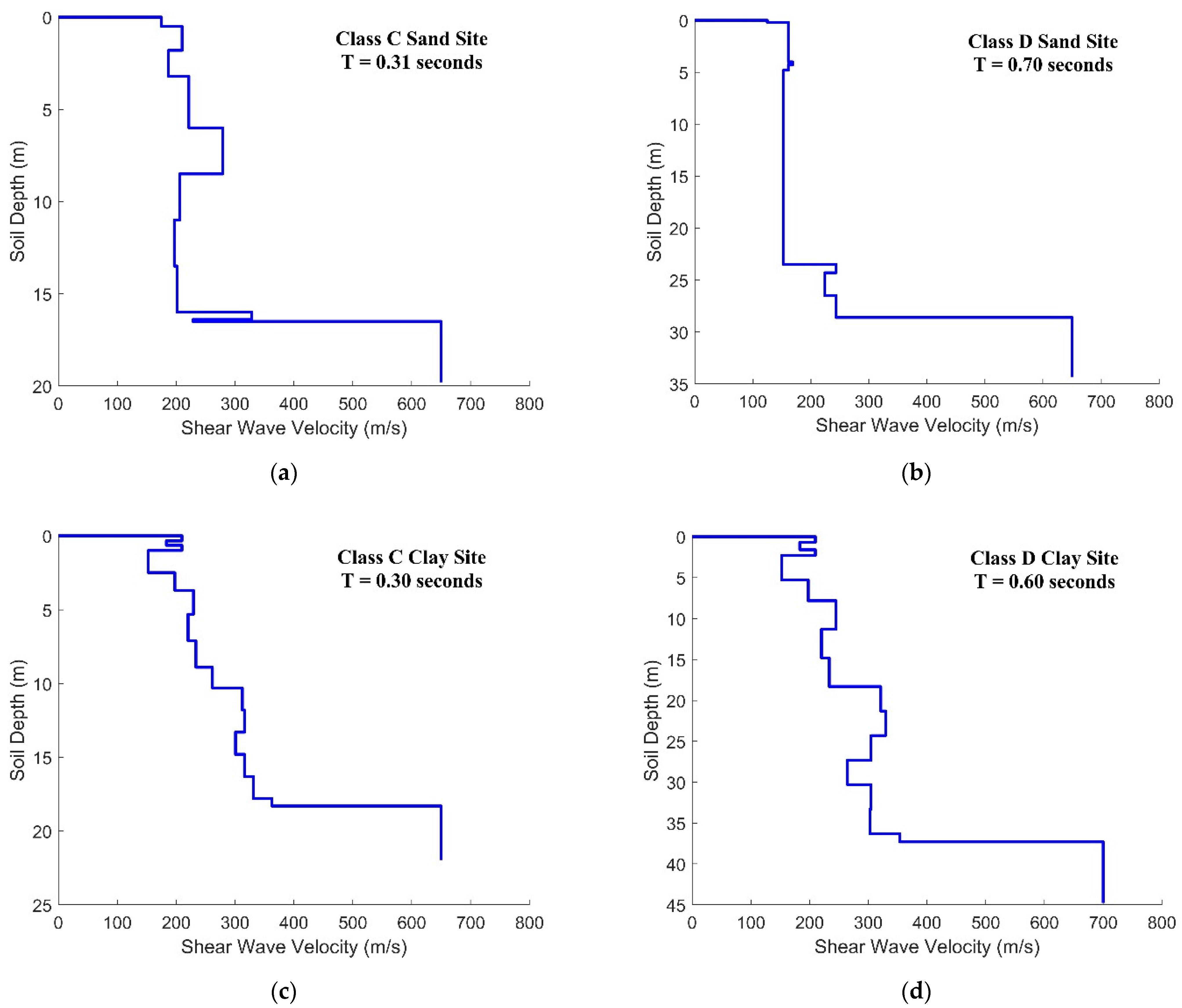
| 1 | 0.31 | Ce | 16.5 | 214.2 | Sydney | Cohesionless | Medium-depth soil site of dense silty sand underlain by sandstone |
| 2 | 0.41 | Ce | 25.95 | 254.3 | Melbourne | Cohesionless | Medium-depth soil site of mixture of silty and clayey sand underlain by hard basalt |
| 3 | 0.60 | De | 30 | 199.6 | Melbourne | Cohesionless | Deep soil site of clayed sand underlain by basalt |
| 4 | 0.70 | De | 28.6 | 164.2 | New Castle | Cohesionless | Medium-depth soil site with 23.5 m loose sand and 5.1 m of medium dense gravel underlain by tuff and sandstone |
| 5 | 0.93 | Ee | 50.5 | 217.0 | Melbourne | Cohesionless | Very deep soil site of wet poorly graded sand underlain by sandstone |
| 6 | 0.18 | Ce | 9.55 | 207.2 | Melbourne | Cohesive | Shallow soil site of soft-to-stiff sandy clay (medium plasticity) underlain by siltstone |
| 7 | 0.30 | Ce | 18.3 | 246.4 | Melbourne | Cohesive | Medium-depth soil site with 3.7 m firm clay and 14.6 m very stiff clay (low plasticity) underlain by siltstone |
| 8 | 0.60 | De | 37.3 | 246.6 | Melbourne | Cohesive | Deep soil site of stiff-to-hard wet clay (low plasticity) underlain by sandstone |
| 9 | 0.67 | De | 33.5 | 199.3 | Brisbane | Cohesive | Deep soil site of stiff clay (high plasticity) underlain by medium strength phyllite; 4.25 m of very soft clay found at 6 m depth |
| 10 | 0.84 | De | 42.5 | 202.2 | Brisbane | Cohesive | Deep soil site of soft-to-stiff clay (high plasticity) underlain by medium strength phyllite |
| 11 | 0.16 | Ce | 9 | 221.3 | Brisbane | Mixture | Shallow layer with 2 m fill sand and clay and 7 m of firm-to-hard clay underlain by basalt |
| 12 | 0.21 | Ce | 13.8 | 257.7 | Brisbane | Mixture | Shallow soil site of a mixture of sand and stiff clay underlain by basalt |
| 13 | 0.35 | Ce | 19.9 | 228.2 | Melbourne | Mixture | Medium-depth soil site with 10 m of stiff cohesive soil and 12 m of mixture of silt and extremely weathered basalt underlain by siltstone |
| 14 | 0.40 | Ce | 30.6 | 305.1 | Melbourne | Mixture | Deep soil site with 16 m of cohesive soil, 14 m of dense sand underlain by sandstone and 2 m of extremely weathered basalt found at 8 m depth |
| 15 | 0.46 | Ce | 23.4 | 203.7 | Sydney | Mixture | Medium-depth soil site of silt and sand underlain by sandstone |
| 16 | 0.51 | Ce | 29.3 | 230.1 | New Castle | Mixture | Medium-depth soil site with 11 m dense sand and 12 m of very stiff clay underlain by sandstone |
| 17 | 0.64 | De | 32.5 | 203.6 | Brisbane | Mixture | Deep soil site with 18 m of soft-to-stiff clay and 14 m of dense sand underlain by low-to-medium strength phyllite |
| 18 | 0.73 | De | 27.6 | 150.7 | Melbourne | Mixture | Very deep soil site with 30 m of cohesive soil and 25 m of dense sand underlain by sandstone |
| 19 | 0.80 | De | 61.2 | 305.1 | New Castle | Mixture | Medium-depth soil site with 3 m fill of gravel, 3 m of organic matters, 9 m of loose sand and 12 m of stiff clay underlain by tuff |
| 20 | 0.97 | Ee | 60 | 247.5 | Melbourne | Mixture | Very deep soil site of mixture of sand and hard clay underlain by hard basalt |
Disclaimer/Publisher’s Note: The statements, opinions and data contained in all publications are solely those of the individual author(s) and contributor(s) and not of MDPI and/or the editor(s). MDPI and/or the editor(s) disclaim responsibility for any injury to people or property resulting from any ideas, methods, instructions or products referred to in the content. |
© 2023 by the authors. Licensee MDPI, Basel, Switzerland. This article is an open access article distributed under the terms and conditions of the Creative Commons Attribution (CC BY) license (https://creativecommons.org/licenses/by/4.0/).
Share and Cite
Hu, Y.; Khatiwada, P.; Tsang, H.-H.; Menegon, S. Site-Specific Response Spectra and Accelerograms on Bedrock and Soil Surface. CivilEng 2023, 4, 311-332. https://doi.org/10.3390/civileng4010018
Hu Y, Khatiwada P, Tsang H-H, Menegon S. Site-Specific Response Spectra and Accelerograms on Bedrock and Soil Surface. CivilEng. 2023; 4(1):311-332. https://doi.org/10.3390/civileng4010018
Chicago/Turabian StyleHu, Yiwei, Prashidha Khatiwada, Hing-Ho Tsang, and Scott Menegon. 2023. "Site-Specific Response Spectra and Accelerograms on Bedrock and Soil Surface" CivilEng 4, no. 1: 311-332. https://doi.org/10.3390/civileng4010018
APA StyleHu, Y., Khatiwada, P., Tsang, H.-H., & Menegon, S. (2023). Site-Specific Response Spectra and Accelerograms on Bedrock and Soil Surface. CivilEng, 4(1), 311-332. https://doi.org/10.3390/civileng4010018