1. Introduction
Air conditioning has provided thermal comfort to building users for many years; this process entails cooling the internal environment to a lower set point than that of the external environment. According to statistics [
1], air conditioning (A/C) uses 20% of the total global electricity in buildings, which equates to an estimated annual 1 trillion kilowatt hours [
2]. This demand is continuously increasing, partially due to global warming [
3]. The International Energy Agency estimates that the global cooling demand could triple by 2050, with a large increase in A/C ownership expected in India and China, consuming as much additional electricity as all of present-day India and China combined [
1]. By means of modelling predictions, Isaac and Vuuren [
4] indicated that electrical demand for A/C will peak in 2020–2030 with an estimated average 7% increase per year. These figures indicate the importance of building elements to be carefully selected and A/C systems to be precisely sized to minimise carbon emissions. To ensure this, heat gain assessment needs to be carried out to determine cooling loads [
5]. In the calculation of cooling loads, a heat balance equation is needed that is derived from numerical models [
6]. There are numerous models that are used, and were developed to ensure that they are universally applicable and have improved accuracy [
7]. Although these models only provide an estimate, a relevant degree of accuracy should be achieved within their processes by using key contributing variables and a certain degree of simplicity, so that they can be applied by engineers [
8]. To ensure further progression, it is important that separate models adopt a collaborative approach, so that cooling loads can be universally standardised.
2. CIBSE and ASHRAE Cooling Load Calculation Methods
Chartered Institution of Building Services Engineers (CIBSE) and American Society of Heating, Refrigerating and Air-Conditioning Engineers (ASHRAE) methods are widely adopted globally for cooling load calculation [
9]. In terms of calculation method, CIBSE adopts the admittance method, which is based upon the fundamentals of heat transfer and the calculation procedures being simplified to be able to deal with both steady-state and fluctuating loads [
10]. The ASHRAE, on the other hand, uses radiant time series (RTS) to calculate steady-periodic cooling loads, which are processed by splitting the heat gain components into convective and radiant components [
11]. The ASHRAE RTS method determines heat gain through the building fabric in which the overall periodic heat transfer factor is dominated by the outdoor temperature [
12]. Once the value for the periodic heat transfer factor is determined, it can then be applied to establish the cooling load through the building fabric [
12]. In this calculation, the periodic heat transfer factor takes into account both the internal and external building fabrics, and heat gains are separated into convective and radiant components, while heat conduction is dealt with by using the corresponding radiant time coefficient, in which the temperature values of the past 23 h are used to formulate the conduction heat gain at the current hour [
13]. However, CIBSE’s fabric heat gain is differently modelled from that of the ASHRAE method. CIBSE’s cyclic variation, the admittance method, accommodates for a swing in fabric heat gain that considers fluctuations of the heat energy transmitted to and from the building fabric [
14].
The CIBSE admittance and ASHRAE RTS methods are similar in terms of the actual approach used to determine cooling loads. In the ASHRAE RTS method, a calculation first determines the heat gain, followed by a second calculation that converts the heat gain into a cooling load. This is achieved by considering previous heat gains with the use of radiant time factors [
15]. The CIBSE admittance method is similar, as the first calculation establishes the sensible steady-state heat gains, followed by a cyclic variation that takes into consideration the building fabric properties; an hourly thermal model can then be created due to the incorporation of coefficient and response factors [
16]. However, as mentioned earlier, the ASHRAE RTS method combines radiation and convection heat transfer, which does not accommodate for conduction from the internal environment, which thereby results in overpredictions [
13]. Conductive heat transfer is calculated by using conduction time series (CTS) on the basis of the thermal properties of the building fabric such as the U-value [
17]. Spitler et al. [
13] demonstrated a slight overprediction using the RTS method that lead to significantly higher prediction on buildings with a high window-to-wall ratio. On the other hand, the CIBSE admittance method of using the solar gain factor-based window model underpredicts cooling loads [
10]. Large window areas may result in excessive solar gains and thus require huge amounts of cooling power [
18].
In fact, the CIBSE’s method relies on tabulated data to determine time lags, resulting from correction factors related to the fabric’s properties [
19]. This is seen for heavy or lightweight buildings that use simplistic correction factors, and may not provide a precise result in cooling loads due to the vague associated time lags [
10]. Brembilla et al. [
20] report that part of the inaccuracy is due to cloud coverage being measured by automated ceilometers. When compared to a separation model, the CIBSE admittance method underestimated solar irradiance components by up to 30%, and underpredictions of 16% and 2% were found for global and diffuse horizontal irradiances, respectively. Furthermore, Demetriou [
19] indicated that tabulated cooling loads are computed for a specific thermal weight, location, and orientation of a building, which depends on whether a shading device was applied. Due to solar gains being reliant upon tabulated data, it is of paramount importance that calibration and longitudinal testing or monitoring are carried out to ensure that the published figures are developed and applicable [
21].
This study qualitatively investigates the CIBSE admittance and ASHRAE RTS methods, which have differing approaches, and consequently reveals the performance gaps within the two methods that lead to discrepancies in cooling load calculation. The methods were contrasted to identify their performance by establishing key components that require attention to ensure that both over- and underpredictions of cooling load are restricted. The study identifies both methods’ limitations, and reviews their accuracy and sensitivity, thereby allowing for recommendations. Furthermore, this study provides the necessary background information for future studies to develop an integrated cooling load model, thus increasing accuracy in calculation.
3. Methodology
This research identifies key inaccuracies and discrepancies within the two cooling load calculation methods, namely, CIBSE admittance and ASHRAE RTS, using a mock-up building. It was not within the scope of this study to identify which method was the most accurate, but a parametric test was conducted to further validate the findings of the literature review, and establish where the models can be improved through extensive contrast analysis of the results. In essence, this also contributed to the validity of the previous reviewed studies. The specific methods and procedures of this study are described as follows.
3.1. Building Description
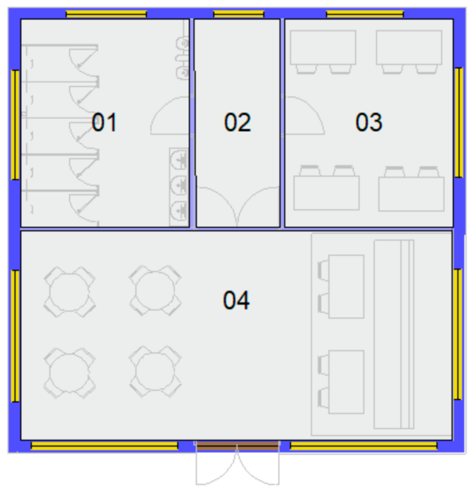
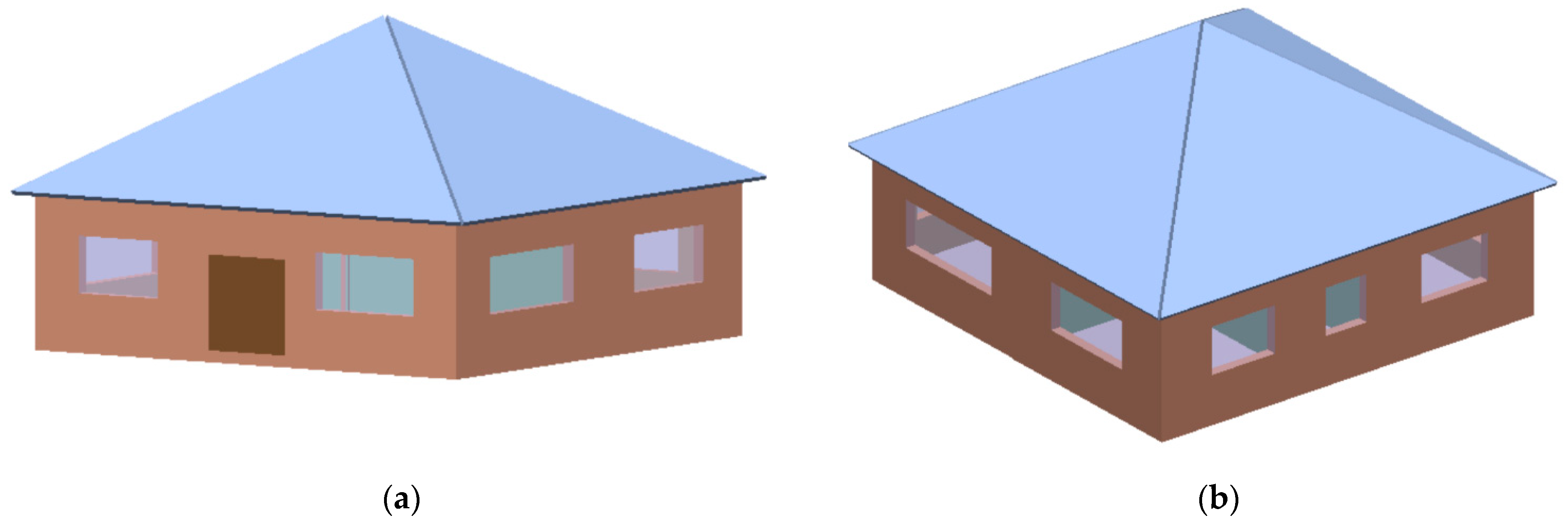
The parametric test between the CBISE admittance and ASHRAE RTS methods was conducted by modelling the peak cooling load for the mock-up building and changing one variable at a time. As shown in
Figure 1 and
Figure 2, the building was single-story, comprising four rooms of various sizes, with the largest room being south-facing.
In order to avoid the interference of the system thermal load, we did not take into account ventilation and infiltration in the proposed test, and the building was assumed to be unconditioned with a zero air change rate (i.e., 0 ACH). Full details of the building’s geometrical and construction information, thermal properties, and design conditions are given in
Table 1,
Table 2 and
Table 3.
3.2. Testing Conditions
Five parameters within this test were independently changed, allowing for transparency when establishing responsiveness and sensitivity to specific aspects. The five parameters are tightly bound to cooling load calculation in either method, as per the literature review. Each test was repeated in three different locations (representing different climate conditions), namely, London, California, and Beijing, with varying degree days, solar irradiance, relative humidity, and temperature. The weather data used within these locations were comparable by using Meteonorm weather source, which is integrated into the used software. Any additional latent or sensible heat gains, such as equipment or people within the building, were neglected to eliminate potential interference. The generated standard building was a medium-weight construction with the thermal properties and materials shown in
Table 2, which remained unchanged throughout all tests. Parameters such as U-values and thermal weights were altered by manually changing these in the software’s global changes options to achieve the desired test values.
Table 4 displays the selected five parameters tested within this study.
3.3. Modelling
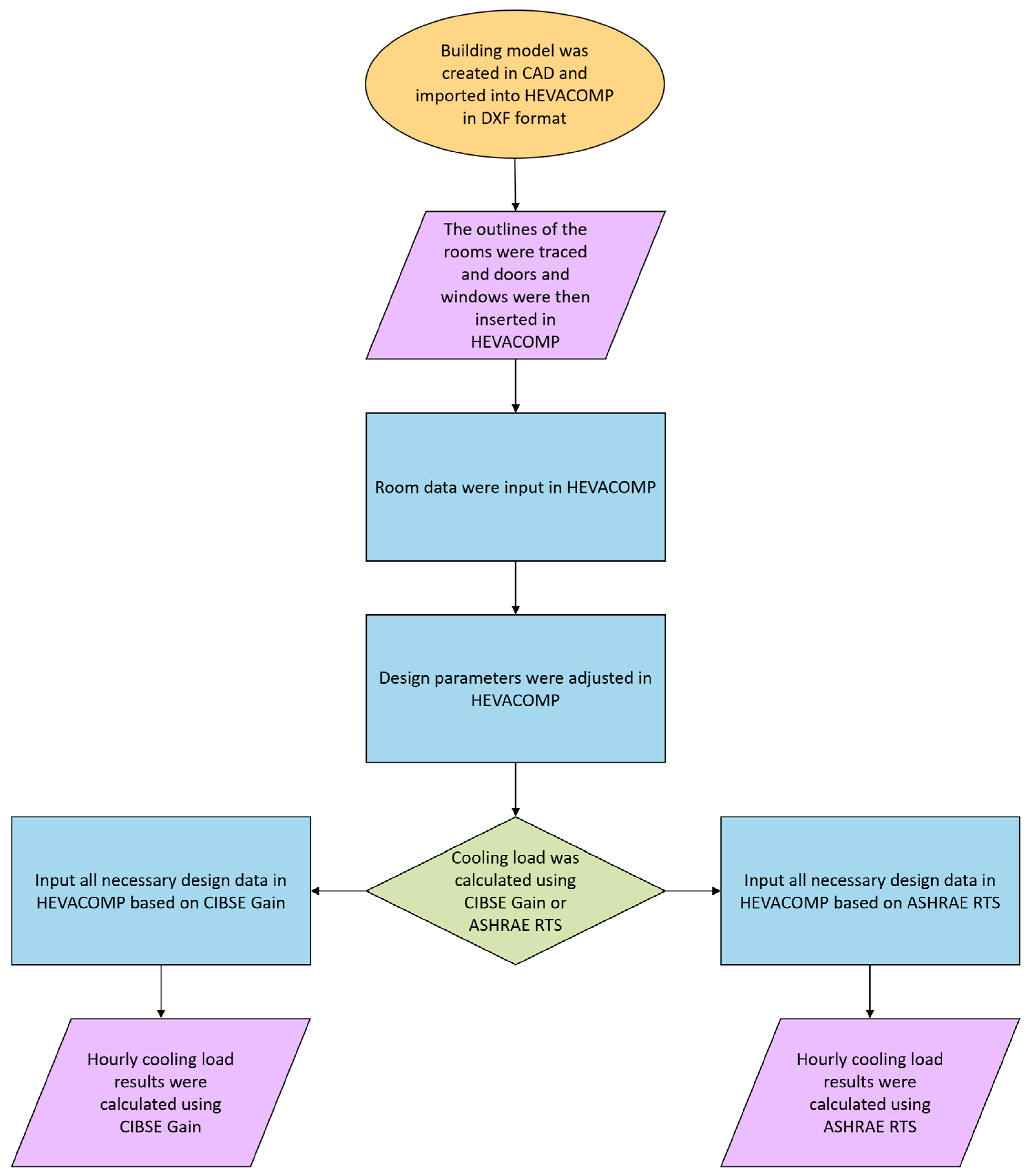
HEVACOMP V8i thermal modelling software was used for this study due to its practicality and accessibility. The mock-up building was initially designed using AutoCAD and imported into the HEVACOMP software in DXF format. The building was then recreated and specific inputs relating to building’s height and properties were selected. The graphical description of the modelling is shown in
Figure 3. Once the building model was created, specific parameters could be adjusted in HEVACOMP. The tests were then ran using the CIBSE Gain (the admittance method) and ASHRAE RTS methods that are integrated into HEVACOMP. Various locations were selected by modifying the building data in the software. Weather data, including the date of peak temperatures, were kept consistent and were automatically selected by the software. A full report of the results could then be displayed with hourly cooling loads. Testing various models through the use of the software and manual calculations with known parameters is widely accepted within thermal analysis studies. For example, Tamm [
22] successfully tested a reduced-order model to validate its ability to determine solar heat gains with different variables such as shading coefficient (SC) and window-to-wall ratio (WWR).
3.4. Organisation
The inputs to the software are user-controlled, so random human error could cause inaccuracies; therefore, precise care was taken. Fields that were automated by the software were accepted and kept consistent throughout all cases. Any anomalies within the results were repeated to improve accuracy. All results were published into an MS Excel spreadsheet, and tables were generated for easy interpretation, as displayed in
Section 4.
4. Results and Discussion
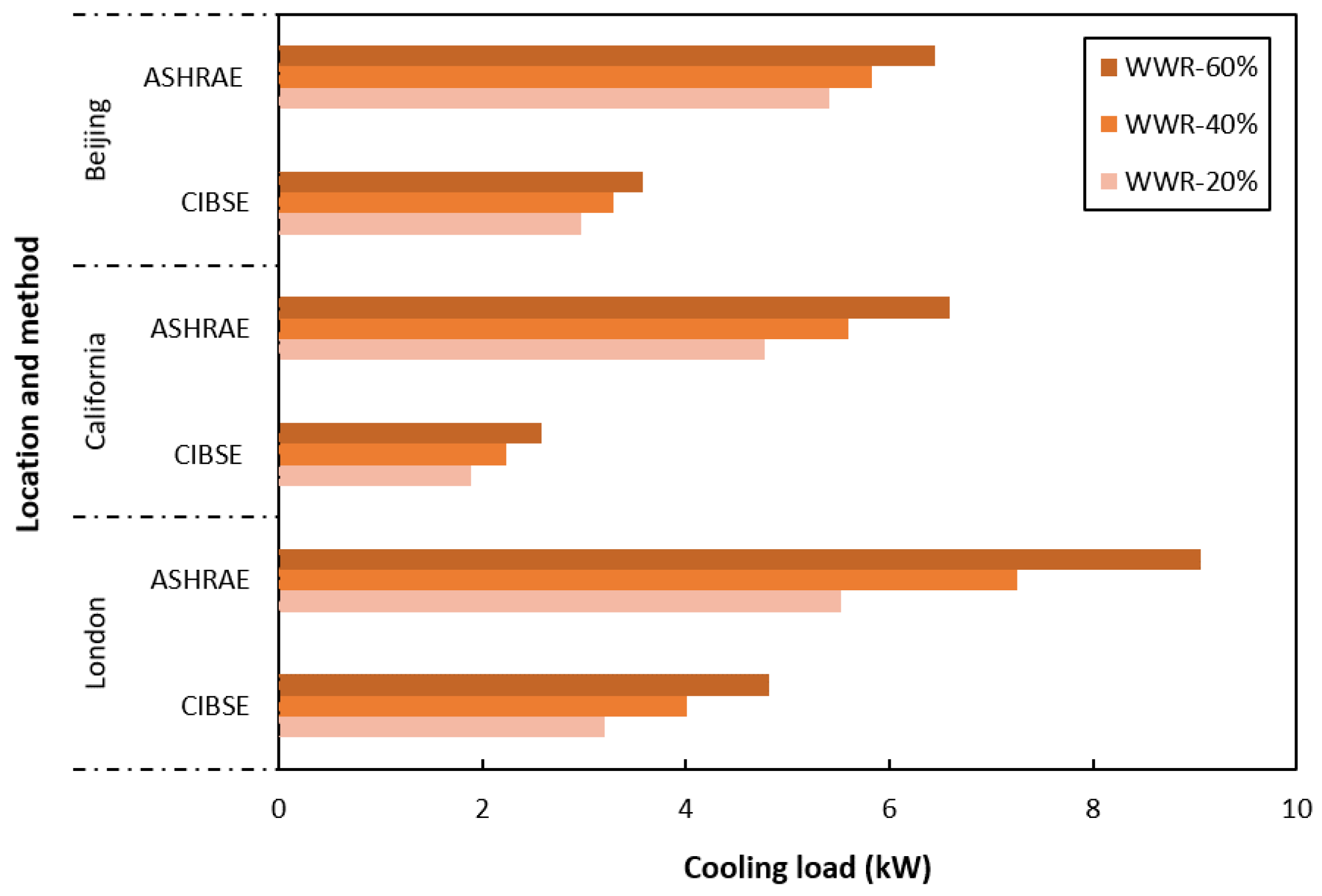
The following figures present the primary results based on the five testing parameters repeated over the three different selected locations. Overall, the most distinctive correlation was that all the tested scenarios showed a higher peak cooling load using the ASHRAE RTS method than that of CIBSE admittance. As discussed in the literature review, there are a number of limitations suggesting that the CIBSE method typically underestimates cooling loads, whereas the ASHRAE method often overpredicts. As shown in
Figure 4, both methods had a distinctive positive correlation to the WWR, but the increments were much greater in the ASHRAE method. For example, results indicate that the 60% WWR in London led to a difference of approximately 4.24 kW between the two methods, which reflected the validity of overprediction in the ASHRAE RTS method.
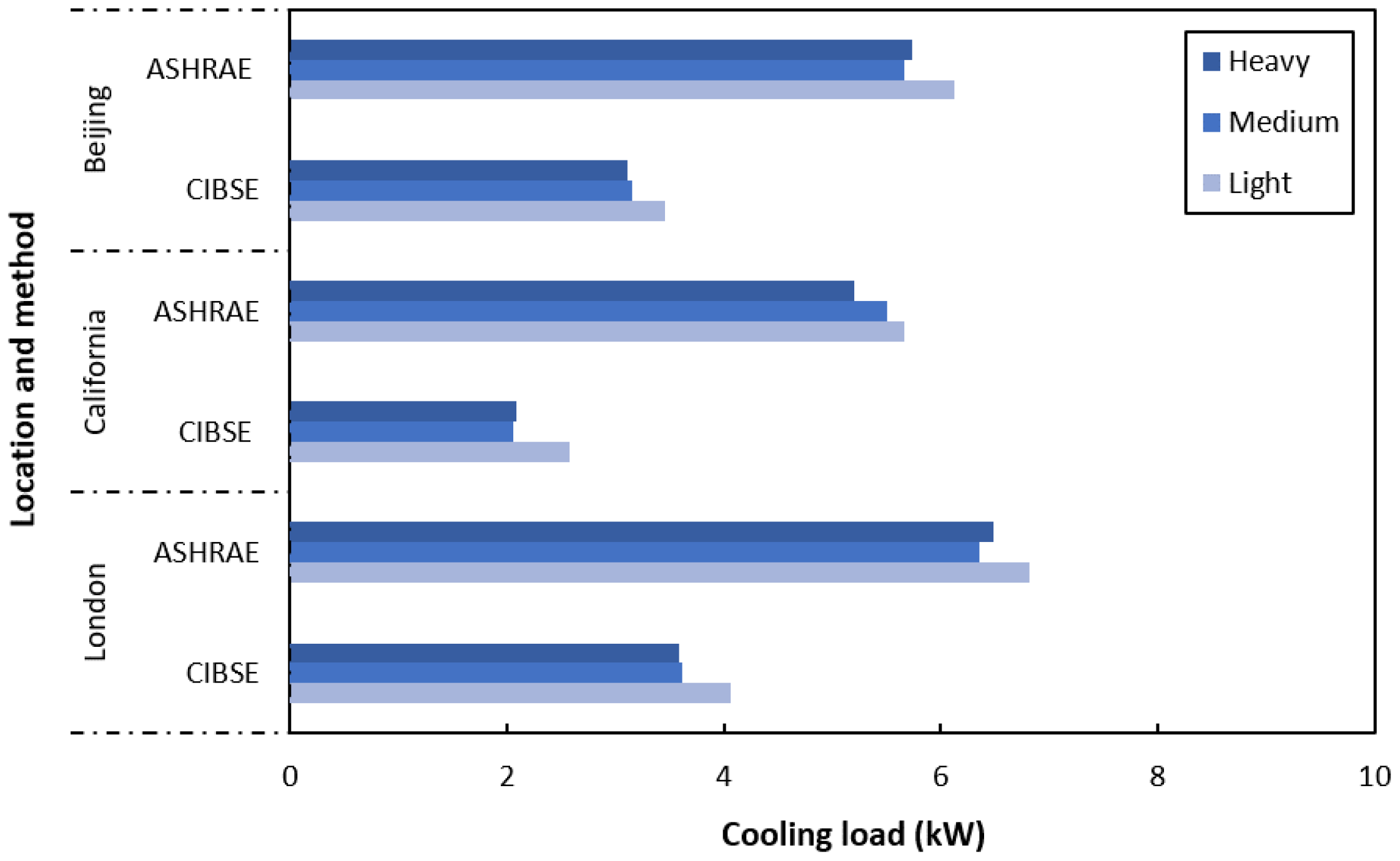
In terms of thermal property, the ASHRAE RTS method also overpredicted the cooling load (
Figure 5 shows). The largest difference between the two methods was when the building’s thermal weight varied, which led to a maximal 62.61% overprediction for the medium weight applied in California. This verified the findings of the literature review that suggested that CIBSE’s tabulated data precisely relating to environmental temperature lag factors are inaccurate and can lead to underpredictions for cooling loads. On the other hand, ASHRAE’s model of using radiant time factors is limited due to its inability to account for losses conducted back to the external environment. That being said, the results show similarities in how both methods were not highly susceptible to variations in the fabric thermal weight. For example, the difference in cooling load between light and heavy thermal mass in California for CIBSE and ASHRAE was about 0.35 and 0.46 kW, respectively. This was most likely due to heat gains to the internal environment being majorly caused by glazed areas. Therefore, although the thermal weight of the building might offset immediate heat gains, peak heat gains remained similar.
Figure 5 also indicates that the majority of results showed a descending trend among light, medium, and heavy weight; however, this differed when comparing ASHRAE’s London and Beijing results. It is most common for this phenomenon to occur due to heavy-weight building material causing the internal temperature to peak at a later time period, but once the internal environment reaches a higher temperature than that of the summer design, room temperatures are likely to remain high for a longer period of time. It is, therefore, reasonable to suggest that ASHRAE’s method of using radiant time factors prolongs the heat gain in comparison to CIBSE’s method for particular instances, independent of location.
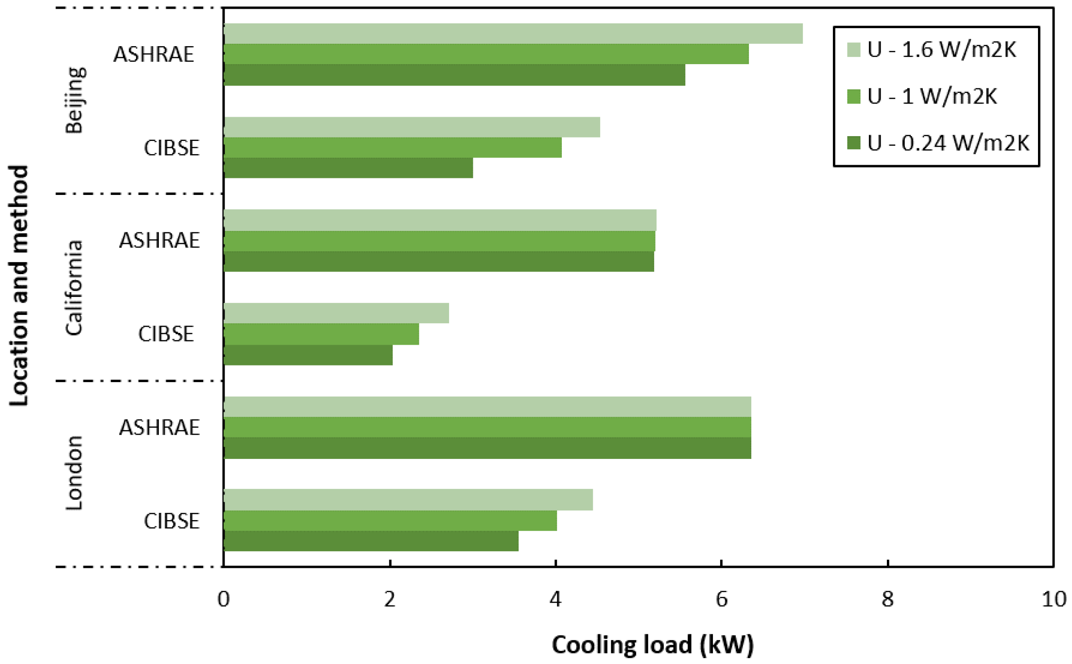
Figure 6 shows, in comparison with CIBSE method, the overpredictions of cooling load that was subject to variation in building fabric U-value using the ASHRAE method. In addition, results show a static figure for the ASHRAE RTS method in London (and even California) for the U-value test, which suggests a malfunction within the software’s logic (i.e., HEVACOMP v8i). This might have been an anomaly in the results, so it was subjected to retesting. However, the outcome remained unchanged by repeating the test. Thus, this part of the test did not display results that were true to ASHRAE’s methodologies.
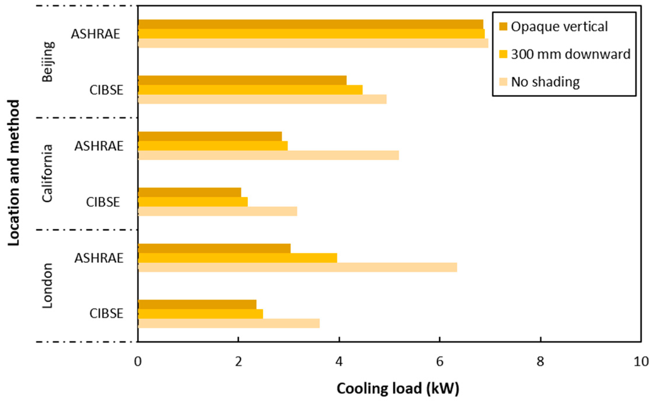
Further, shading device and orientation tests were carried out to examine how solar irradiance upon the glazed area affects the cooling loads.
Figure 7 shows that the use of different shading devices provided results of cooling loads that were close to one another over the three locations, although overprediction was found when using ASHRAE RTS method. The largest difference among the results was found when no shading was used for the ASHRAE calculation, with a maximum of 3.3 kW to the opaque vertical shading in London, while this difference was only about 1.26 kW in the CIBSE calculation.
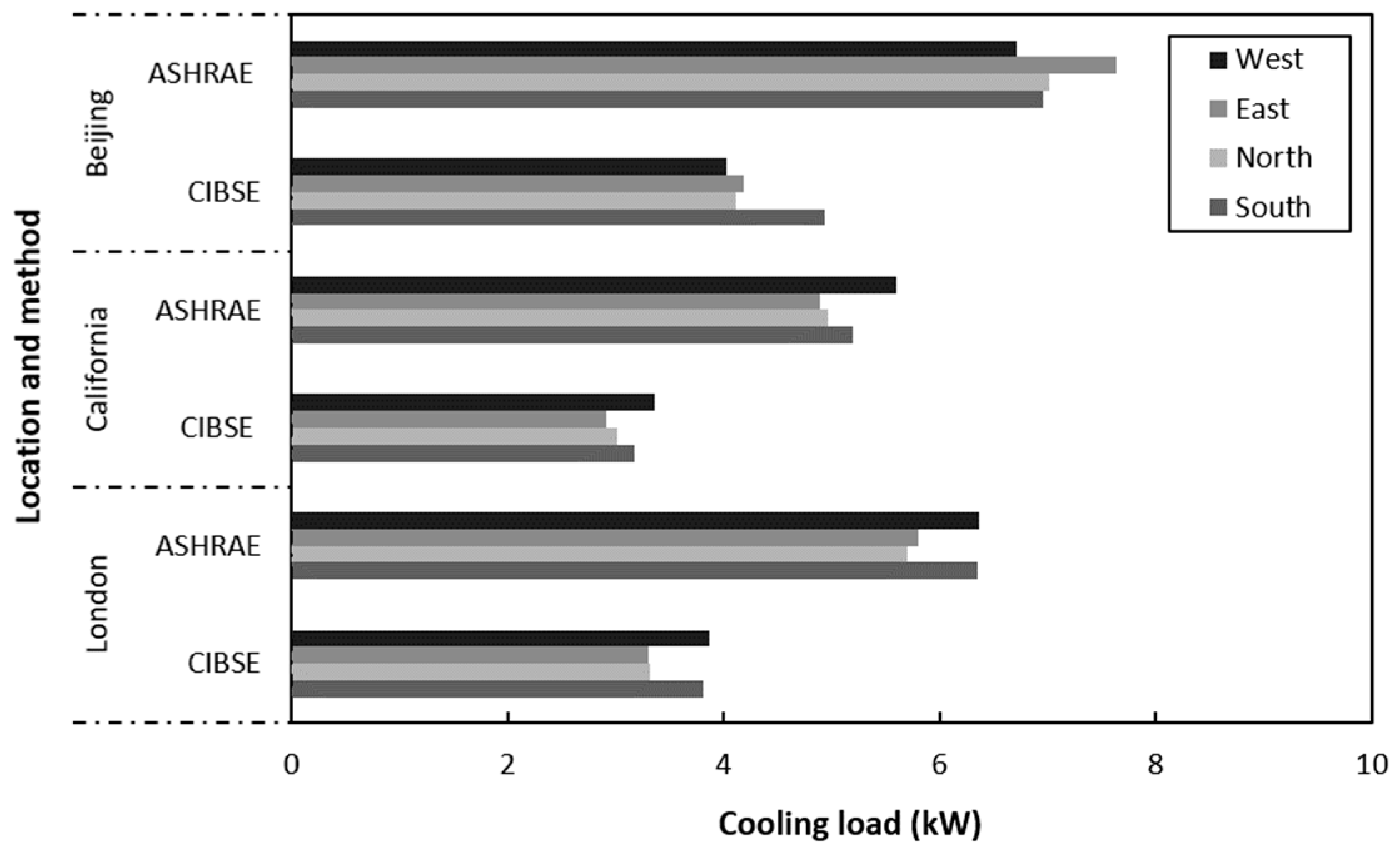
Figure 8 shows that the ASHRAE method predicted a higher cooling load than CIBSE did in regard to orientation for all three locations. This could have been caused by variations in the methods, as ASHRAE uses peak irradiance compared to CIBSE’s mean irradiance values, and because of the accuracy of the tabulated data. The patterns were very similar between the two methods for the London and California cases. However, results show distinct pattern differences for the Beijing case, especially for the higher cooling load predicted by ASHRAE when the building was facing east and north, possibly due to the inaccuracy of weather data.
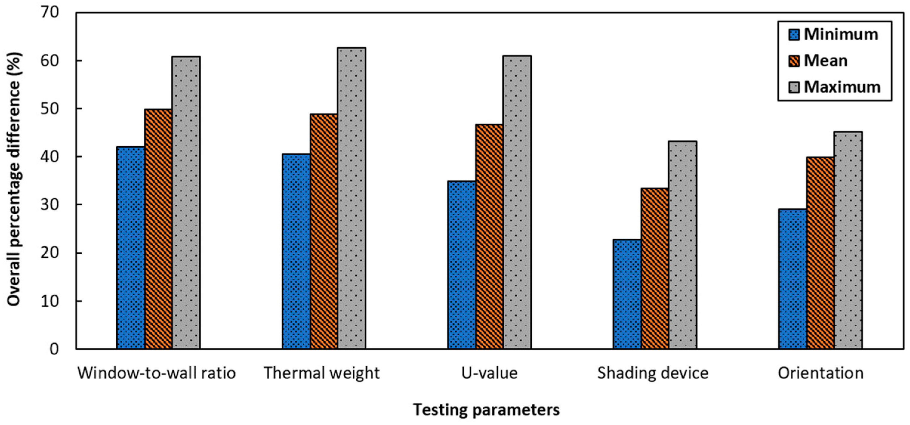
Figure 9 shows the minimal, mean, and maximal percentage differences in peak cooling load between the two methods throughout the five testing parameters. The parameters of WWR and thermal weight both presented the largest difference between the two methods. Both maximal difference due to WWR, and thermal weight between CIBSE and ASHRAE predictions were over 60%. Due to ASHRAE’s RTS method of using peak exterior irradiance and being more vulnerable to higher conductance, this result was as expected.
5. Conclusions
This paper determined following a literature review that consistent historical issues were present with both cooling load prediction methods, CIBSE admittance and ASHRAE radiant time series (RTS). There was clear consistency within the literature that ASHRAE typically overpredicts cooling loads, whereas CIBSE underpredicts them. As discussed, the main variations between the two methods were the way in which building models were dynamically modelled within their calculations. ASHRAE RTS uses radiant time coefficients accounting for previous heat gains for the past 23 h to establish a cooling load. In comparison, CIBSE admittance uses tabulated data to accommodate for fluctuations and storage effects with the use of temperature swings and time lags associated with the decrement factor.
The study demonstrated a parametric test that had been performed by modelling a mock-up building in HEVACOMP v8i software and analysing the cooling load results. Overall, ASHRAE predicted a much larger peak cooling load than the CIBSE method did, with a maximal average difference of over 60%. The ASHRAE model showed much higher extremities to parameter changes, especially with regard to solar radiation on glazed surfaces. Contrary to expectations, there was only a slight total mean difference between the two models responding to a change from light to heavy thermal weight.
As discussed in the literature review, ASHRAE’s limitation is the inability to conduct heat to the external environment; however, this flaw is most extreme in highly conductive materials, unlike the building fabric used within this study. The substantial predicted cooling load difference was caused by solar radiation through the glazed area, and discrepancies were only minor when considering the building fabric. This was further supported by the results of the shading device and window-to-wall ratio tests. When analysing the WWR results, the highest level of discrepancy was seen in the London scenario, where at 20% WWR for the ASHRAE’s model results, it was 5.52 kW, which considerably increased to 9.06 kW for 60% WWR. However, the CIBSE’s model only increased by 1.62 kW. Additionally, the shading device test in London displayed a 3.3 kW decrease in cooling load between no shading and opaque vertical shading using the ASHRAE RTS method. In comparison, the CIBSE’s decrease was 1.26 kW. This indicated that the ASHRAE’s model was highly receptive to solar gains, which was a leading contributor to the ASHRAE’s predictions being much higher in all tests.
Furthermore, the inability of the ASHRAE RTS to take into account heat losses from the internal environment leads to overpredictions of cooling load, which is more questionable when conductive materials are implemented in building fabric. On the other hand, calculations in CIBSE admittance were for a swing in fabric heat gain leading to fluctuations in the heat energy transmitted to and from the building fabric, and the swing external temperature could have been significantly underpredicted, which contributed to reduced cooling load estimates. Thus, it is important that longitudinal data are maintained to provide revised calibrated figures, ensuring relevancy and applicability to various parameters.
6. Limitations and Future Research
The collected data within this test were limited due to its small size; therefore, definitive conclusions could not be reached. However, the results present strong consistency with the previously discussed literature. To solidify the results of this study, a starting point would be to replicate the tests on a larger magnitude, with an increase in parameters such as building configuration, weather conditions, and locations. A larger sample also ensures that errors are less relevant and thereby do not dramatically affect the overall results. To establish clear accuracy for both models (i.e., CIBSE admittance and ASHRAE RTS), a study should be carried out through an in-situ test to establish the actual cooling load for both methods’ predictions. Performing this type of test with a larger sample size requires a longer test, apparatuses, and field trips, which, however, were outside the scope of this paper.
The next decade is a critical period in the fight against climate change; therefore, it is important that equipment is accurately sized to prevent high emission rates and a lack of efficiency [
23]. The two methods in this study showed a large variation in cooling load predictions, meaning that inaccuracy was still present within either or both methods. Further studies may be carried out to establish a collaborative model using CIBSE’s traits to compensate for ASHRAE’s performance gaps discussed above by, for instance, using temperature swings, time lags, and decrement factors rather than radiant time factors.


