Statistical Properties in Jazz Improvisation Underline Individuality of Musical Representation

Abstract

Statistical learning is an innate function in the brain and considered to be essential for producing and comprehending structured information such as music. Within the framework of statistical learning the brain has an ability to calculate the transitional probabilities of sequences such as speech and music, and to predict a future state using learned statistics. This paper computationally examines whether and how statistical learning and knowledge partially contributes to musical representation in jazz improvisation. The results represent the time-course variations in a musician’s statistical knowledge. Furthermore, the findings show that improvisational musical representation might be susceptible to higher- but not lower-order statistical knowledge (i.e., knowledge of higher-order transitional probability). The evidence also demonstrates the individuality of improvisation for each improviser, which in part depends on statistical knowledge. Thus, this study suggests that statistical properties in jazz improvisation underline individuality of musical representation.

1. Introduction

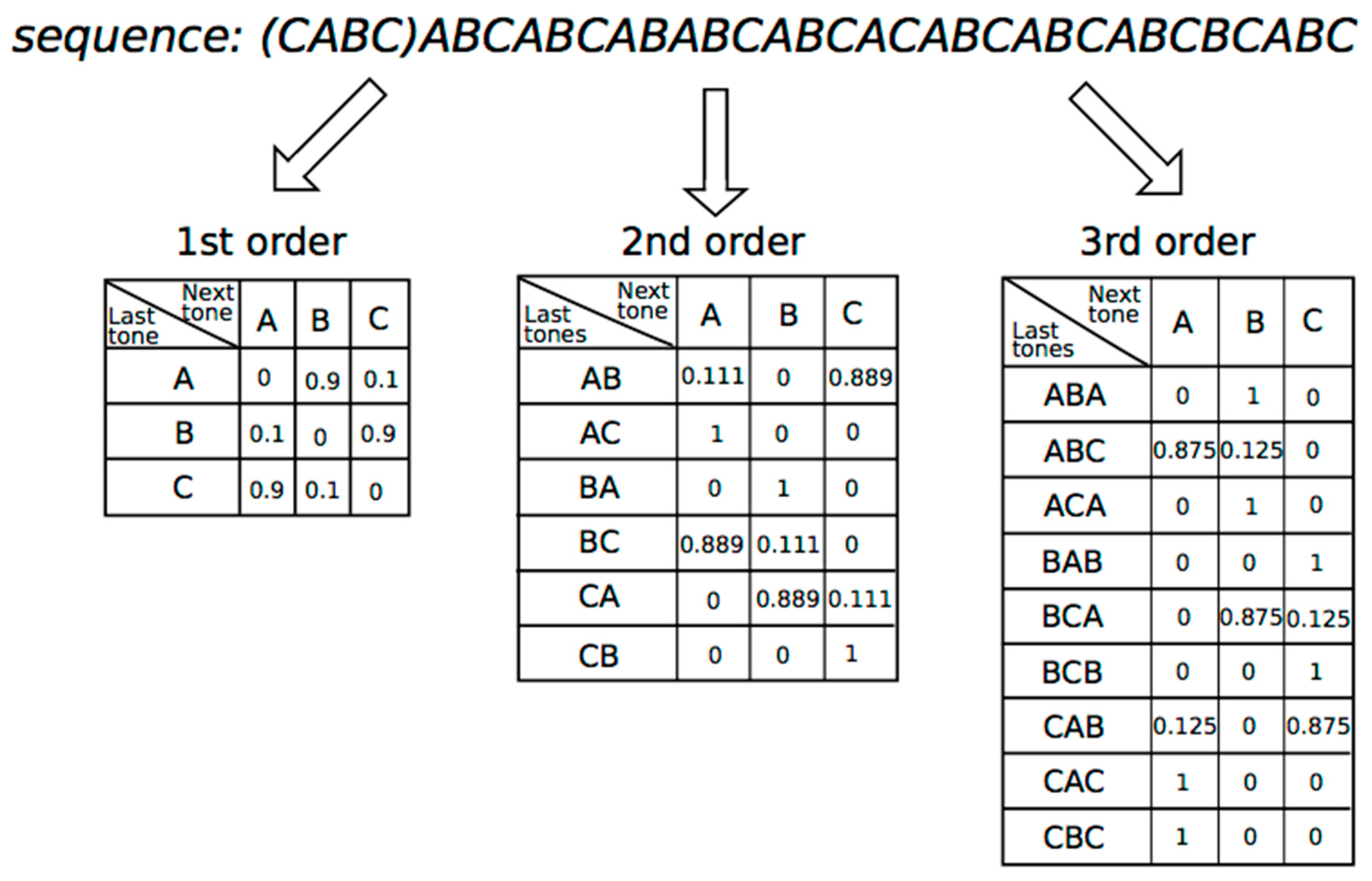
1.1. Statistical Learning: A Mathematical Model of a Learning System in the Brain

According to the hypothesis of statistical learning (SL), our brain has an ability to learn the transitional probabilities (TPs) of sequential information such as speech and music without intention, and predicts a future state using the learned statistical information [1,2,3]. Statistical learning, which occurs even in sleeping neonates and infants [4,5], is considered an implicit and innate system in humans. Evidence has suggested that, even if humans are unaware of what they learn, neurophysiological responses disclose statistical learning effects [6,7,8,9,10,11,12,13]. This learned knowledge can be in part expressed via an abstract medium such as a musical melody [14,15,16]. Thus, statistical knowledge may be reflected in the melodies written by an improviser: a high-probability sequence in music may be one that an improviser is more likely to choose, while creative artists are capable of producing low-probability (i.e., novel, unexpected) improvisations. Indeed, statistical learning has been applied to develop an automatic composition system that gives to computers learning and creative ability similar to those of the human brain [17]. The statistical-learning model is often expressed by the Markov process in which the probability of the forthcoming state is statistically defined only by the latest state, as in the information theory framework of Claude Shannon [18], including the use of n-grams to estimate the statistical structure of environmental information, and the development of entropy as a quantitative measure of the predictability of information [19]. Using multi-order Markov stochastic models, some researchers have also investigated the relationships between human statistical knowledge and statistical structure in music [20,21,22,23]. It has been suggested that the musical creativity of humans in part depends on the statistical learning that occurs in the brain [24,25,26,27].

1.2. Corpus Study in Music: Classical and Jazz Music

Music has numerous domain-specific structures (e.g., tonal pitch spaces, hierarchical tension, attraction contours) [28,29]. This suggests that statistical learning may be inadequate as a model of human music composition. Indeed, improvisers acquire extensive music-specific knowledge such as knowledge of harmonics and musical grammar, and intentionally follow these theories when composing music. The characteristics inherent in music can be revealed by referring to music-specific structures, such as harmonics and tonalities, in musical scores. This suggests that musical knowledge underlying composition strategies can be extracted based on music’s specificity. On the other hand, it has been suggested that musicians access their statistical knowledge when composing music [20,21,22,23]. It is of note, however, that we cannot exclude the possibility that pitch choices during improvisation may strongly depend on aesthetic preferences involved in domain-specific and long-term musical knowledge such as tonality, as well as learned transition probabilities, although it is difficult to empirically reveal these effects because long-term exposure to music is hard to measure. Nonetheless, in jazz music, at least compared to other types of musical composition, in which an improviser deliberates and refines a composition scheme for a long time based on musical theory, musicians are forced to immediately play their own music, partially using long-term training associated with procedural learning [30,31,32,33]. Thus, the performance of musical improvisation is intimately bound to statistical knowledge because of the necessity of intuitive decision-making [34,35,36] and auditory-motor planning based on procedural knowledge. To understand the relationships between improvisational musical representation and statistical knowledge, it is important to examine the stochastic structure embedded in musical improvisation. According to previous studies, the brain codes the statistics of auditory sequences as relative information such as distribution of relative-pitch frequencies, and this information can be used in the comprehension of other sequential structures [7,8]. Thus, this study investigates distribution of relative-pitch frequencies (i.e., pitch interval) in music. This procedure has the advantage also of eliminatng the effects of differences in key on transitional patterns. The present study examines how TP of sequence associated with relative but not absolute pitch is distributed in improvisation.

1.3. Computational Modeling of Musical Improvisation

According to SL theory, the brain automatically computes TP distributions in sequential phenomena. The TP distributions sampled from sequential information such as music are often expressed by nth-order Markov models. The nth-order Markov model is based on the conditional probability of an element e_n+1 given the preceding n elements:

$$P\left(e_{n+1}|e_n\right)=\frac{P\left(e_{n+1}{{\displaystyle \cap }}^{}{e}_n\right)}{P\left(e_n\right)}$$

(1)

From the viewpoint of Psychology, the formula can be interpreted as positing that the brain predicts a subsequent event e_n+1 based on the preceding events in a sequence. In other words, learners expect the event with the highest TP based on the latest n states, whereas they are likely to be surprised by an event with lower TP. The TPs of all transition patterns in a piece of music can be expressed by a TP matrix (Figure 1).

1.4. Study Purpose

The purpose of the present study is to examine the statistical structure embedded in musical improvisation based on various-order hierarchical models of TPs, and to reveal the statistical differences among improvisers. The TPs of melody in pieces of improvisational music played by Bill Evans, McCoy Tyner, and Herbert Jeffrey Hancock (hereafter, Herbie Hancock) were calculated based on nth-order Markov models (Figure 2). In Study 1, using the TPs, information contents (I) were calculated in the framework of information theory. In previous studies, information contents could be regarded as surprising or predictable. In other words, lower information contents mean higher predictabilities and smaller contents mean more surprise, whereas higher information contents mean lower predictabilities and larger surprise [37,38,39,40,41]. From the psychological perspective, a tone with lower information content based on a TP may be one that an improviser is more likely to predict and choose as the next tone, compared to tones with higher information contents. Thus, information content can be used in computational studies of music to discuss psychological phenomena involved in prediction and statistical learning. Information contents based on TPs were compared among improvisers and sequences. It was hypothesized that statistical similarity may represent common styles which all improvisers shared, whereas statistical differences among improvisers may represent the specific characteristics of each improviser. In Study 2, chronological variations of the TPs were investigated. It was hypothesized that there may be two types of chronological variation: TPs that gradually decrease, and those that gradually increase, consistent with chronological order. If so, these findings suggest that statistical knowledge in music gradually shifts over a composer’s lifetime. Second, differences in the statistical structure between musicians and between pieces of music were examined. It was hypothesized that there were statistical characteristics shared between different musicians and between pieces of music. If so, these findings suggest that statistics embedded in musical improvisation may represent individualities of musical expression.

2. Study 1

2.1. Methods

We used the improvisational sequences of the highest pitches from 21 pieces of music played by three improvisors (i.e., 7 improvisations per performer,

Table 1. Music sample used in the present study.

Improvisors	Titles
W. J. Evans	Autumn Leaves from Portrait in Jazz, 1959
	Israel from Explorations, February 1961
	I Love You Porgy from Waltz for Debby, June 1961
	Stella by Starlight from Conversations with Myself, 1963
	Who Can I Turn To from Bill Evans at Town Hall, 1966
	Some Day My Prince Will Come from the Montreux Jazz Festival, 1968
	A Time for Love from Alone, 1969
H. J. Hancock	Cantaloupe Island from Empyrean Isles, 1964
	Maiden Voyage from Flood, 1975
	Some Day My Prince Will Come from The Piano, 1978
	Dolphin Dance from Herbie Hancock Trio ’81, 1981
	Thieves in the Temple from The New Standard, 1996
	Cotton Tail from Gershwin’s World, 1998
	The Sorcerer from Directions in Music, 2001
M. Tyner	Man from Tanganyika from Tender Moments, 1967
	Folks from Echoes of a Friend, 1972
	You Stepped Out of a Dream from Fly with the Wind, 1976
	For Tomorrow from Inner Voice; 1977
	The Habana Sun from The Legend of the Hour, 1981
	Autumn Leaves from Revelations, 1988
	Just in Time from Dimensions from Dimensions, 1984

). The present study only analyzed the highest pitch because the definition of melody in each title is still controversial in musicological study, as different melodies could concurrently appear in different titles of music, and melody is often played at the highest pitches. The TPs of sequences at the highest pitches were calculated based on five different hierarchical models. The probability of a forthcoming tone was statistically defined by the last tone to five successive tones, respectively (i.e., first- to fifth-order Markov chains). For each type of pitch transition, all pitches were numbered so that the first pitch was 0 in each transition, and an increase or decrease in a semitone was 1 and −1 based on the first pitch, respectively. This reveals how the pitches, but not the notes, transitioned from the first pitch. For example, the transition of C5, D5, E5, F5, and B4 was numbered 0, 2, 4, 5, and −1. This procedure was employed to eliminate the effects of the change of key on transitional patterns. Each transition pattern was chronologically ordered based on the time courses in which music was played by each musician. Using the transitional patterns that appear in all pieces of music, the time-course variations of the TPs were analyzed by multiple regression analyses using the stepwise method. The criteria of the variance inflation factor (VIF) and condition index (CI) were set at VIF < 2 and CI < 20 to confirm that there was no multi-collinearity. The VIF is a measure of the effect of other predictor variables on a regression coefficient. CI represents the collinearity of combinations of variables in the data set (actually the relative size of the eigenvalues of the matrix). Using TP matrices in music, each statistical characteristic was compared by Kendall’s tau coefficient analysis. The criteria of the eigenvalue were set above 1. Furthermore, the TPs were weight-averaged in all pieces of music for each musician and for all musicians. Using the weight-averaged TP matrices for each musician, statistical characteristics were compared among musicians by correlation analysis. The representative phrases of transition patterns with the highest probabilities for each musician were decoded as music scores. Statistical significance levels were set at p = 0.05 for all analyses.

2.2. Results

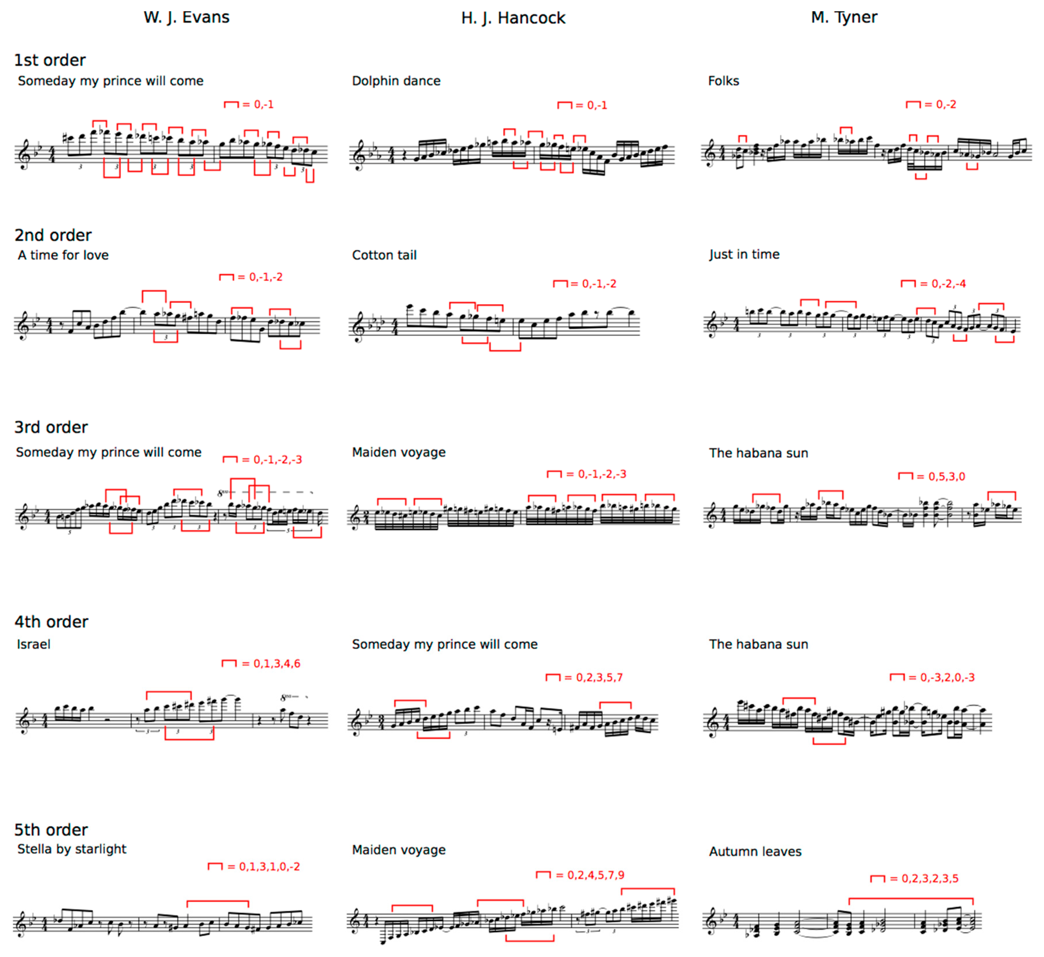
2.2.1. Time-Course Variation in Musical Improvisation

W. J. Evans

Fifteen transitional patterns with two tones that appear in all pieces of music were detected ((0,0), (0,1), (0,−1), (0,10), (0,2), (0,−2), (0,3), (0,−3), (0,4), (0,−4), (0,5), (0,−5), (0,7), (0,8), and (0,−8)). Using these transitional patterns, a multiple linear regression was carried out to predict the chronological order in which music is played by each musician, based on the TPs of the 15 transitional patterns. No significant regression equation was detected, however. Forty transitional patterns with three tones that appear in all pieces of music were detected ((0,−1,0), (0,1,−1), (0,−1,−1), (0,1,2), (0,1,−2), (0,−1,2), (0,−1,−2), (0,1,3), (0,1,−3), (0,−1,−3), (0,1,4), (0,1,5), (0,2,0), (0,−2,0), (0,−2,−1), (0,2,3), (0,−2,−3), (0,2,4), (0,−2,−4), (0,−2,−5), (0,−2,−6), (0,−2,−7), (0,3,0), (0,3,1), (0,−3,−1), (0,3,2), (0,−3,−2), (0,−3,−4), (0,−3,−5), (0,3,6), (0,−3,−6), (0,3,7), (0,−3,−7), (0,4,5), (0,−4,−5), (0,4,7), (0,−4,−7), (0,5,3), (0,−5,−9), and (0,7,4)). Using these transitional patterns, a multiple linear regression was carried out to predict the chronological order in which music was played by each musician, based on the TPs of the 40 transitional patterns. No significant regression equation was detected, however. Sixteen transitional patterns with four tones that appear in all pieces of music were detected ((0,−1,−2,−3), (0,1,3,1), (0,1,3,4), (0,−1,−3,−4), (0,1,5,8), (0,−2,0,−2), (0,−2,−1,−3), (0,2,3,5), (0,−2,−3,−5), (0,2,4,5), (0,−2,−5,−9), (0,−2,−7,−11), (0,−3,−2,2), (0,−3,−4,−6), (0,−3,−7,−10), and (0,4,7,11)). Using these transitional patterns, a multiple linear regression was carried out to predict the chronological order in which music was played by each musician, based on the TPs of the 16 transitional patterns. A significant regression equation was found (F(2,4) = 12.71, p = 0.018), with an adjusted R2 of 0.80 (

Table 2. Summary of multiple regression analyses carried out with the stepwise method to predict the chronological order in which music is played by each musician based on the TPs.

a. W. J. Evans
		Model 1					Model 2
Hierarchy	Variable	B	SE B	β	VIF	CI	B	SE B	β	VIF	CI
Third	0,2,3,5	−171.28	66.20	−0.76 *	1.00	4.08	−144.06	42.75	−0.64 *	1.05	3.33
	0,−3,−4,−6						627.99	214.37	0.55 *	1.05	6.85
	R2	0.49					0.80
	F	6.69 *					12.71 *
Forth	0,1,3,4,6	−317.34	97.30	−0.83 *	1.00	3.92
	R2	0.62
	F	10.64 *
b. M. Tyner
		Model 1					Model 2
Hierarchy	Variable	B	SE B	β	VIF	CI	B	SE B	β	VIF	CI
Second	0,−2,−5	172.15	38.79	0.89 **	1.00	6.37	191.08	20.78	0.99 **	1.06	5.51
	0,5.7						−485.35	127.57	−0.41 *	1.06	7.89
	R2	0.76					0.93
	F	19.70 **					43.63 **

* p < 0.05 ** p < 0.01; SE = standard error, VIF = variance inflation factor, CI = condition index.

a). The predicted chronological order is equal to 4.12–144.06 (transition of (0,2,3,5)) + 627.99 (transition of (0,−3,−4,−6)). The TPs of (0,2,3,5) and (0,−3,−4,−6) gradually decreased and increased consistently with the chronological order, respectively ((0,2,3,5) p = 0.028, (0,−3,−4,−6) p = 0.043). These TPs were significant predictors of chronological order.

Four transitional patterns with five tones that appear in all pieces of music were detected ((0,−1,−2,−3,−4), (0,1,3,4,6), (0,1,5,8,12), and (0,−3,−2,2,5)). Using these transitional patterns, a multiple linear regression was carried out to predict the chronological order in which music is played by each musician, based on the TPs of the four transitional patterns. A significant regression equation was found (F(1,5) = 12.71, p = 0.022), with an adjusted R2 of 0.62 (Table 2a). The predicted chronological order is equal to 7.02–317.34 (transition of (0,1,3,4,6)). The TPs of (0,1,3,4,6) gradually decreased consistently with the chronological order (p = 0.022). These TPs were significant predictors of the chronological order. Transitional patterns with six tones that appear in all pieces of music were detected ((0,−3,−2,2,5,9)). Using these transitional patterns, a multiple linear regression was carried out to predict the chronological order in which music is played by each musician, based on the TPs of the transitional pattern. No significant regression equation was detected, however.

H. J. Hancock

Sixteen transitional patterns with two tones that appear in all pieces of music were detected ((0,0), (0,1), (0,−1), (0,2), (0,−2), (0,3), (0,−3), (0,4), (0,−4), (0,5), (0,−5), (0,6), (0,7), (0,−7), (0,9), and (0,−9)). Using these transitional patterns, a multiple linear regression was carried out to predict the chronological order in which music was played by each musician, based on the TPs of the 16 transitional patterns. No significant regression equation was detected, however. Nineteen transitional patterns with three tones that appear in all pieces of music were detected ((0,0,0), (0,1,0), (0,−1,−3), (0,2,0), (0,−2,0), (0,−2,−2), (0,2,4), (0,−2,−4), (0,2,5), (0,−2,−5), (0,−2,−7), (0,3,0), (0,3,5), (0,−3,−5), (0,3,7), (0,4,2), (0,−4,−7), (0,5,0), and (0,5,3)). Using these transitional patterns, a multiple linear regression was carried out to predict the chronological order in which music was played by each musician, based on the TPs of the 19 transitional patterns. No significant regression equation was detected, however. Transitional patterns with four tones that appear in all pieces of music were detected ((0,1,0,−2)). Using these transitional patterns, a multiple linear regression was carried out to predict the chronological order in which music was played by each musician, based on the TPs of the transitional pattern. No significant regression equation was detected, however. No transitional patterns with five or more tones that appear in all pieces of music were detected.

M. Tyner

Seventeen transitional patterns with two tones that appear in all pieces of music were detected ((0,0), (0,1), (0,−1), (0,10), (0,2), (0,−2), (0,3), (0,−3), (0,4), (0,−4), (0,5), (0,−5), (0,6), (0,−6), (0,7), (0,−7), and (0,8)). Using these transitional patterns, a multiple linear regression was carried out to predict the chronological order in which music was played by each musician, based on the TPs of the 17 transitional patterns. No significant regression equation was detected, however. Thirty-two transitional patterns with three tones that appear in all pieces of music were detected ((0,0,0), (0,1,3), (0,2,0), (0,−2,0), (0,−2,−2), (0,2,3), (0,−2,3), (0,−2,−3), (0,2,4), (0,−2,−4), (0,2,5), (0,−2,−5), (0,2,7), (0,−2,−7), (0,3,0), (0,−3,0), (0,3,1), (0,−3,2), (0,−3,−3), (0,3,5), (0,−3,−5), (0,−3,−6), (0,3,7), (0,−3,−7), (0,4,2), (0,−4,−2), (0,4,7), (0,−4,−7), (0,5,2), (0,5,3), (0,5,5), and (0,5,7)). Using these transitional patterns, a multiple linear regression was carried out to predict the chronological order in which music was played by each musician, based on the TPs of the 32 transitional patterns. A significant regression equation was found (F(2,4) = 43.63, p = 0.002), with an adjusted R2 of 0.93 (Table 2b). The predicted chronological order is equal to –0.12 + 191.08 (transition of (0,−2,−5)) − 485.35 (transition of (0,5,7)). The TPs of (0,−2,−5) and (0,5,7) gradually increased and decreased consistently with the chronological order, respectively ((0,−2,−5) p = 0.001, (0,5,7) p = 0.019). These TPs were significant predictors of the chronological order. Seven transitional patterns with four tones that appear in all pieces of music were detected ((0,2,4,2), (0,−2,−5,−9), (0,3,5,3), (0,−3,−5,−7), (0,−3,−7,−5), (0,4,2,0), and (0,5,3,0)). Using these transitional patterns, a multiple linear regression was carried out to predict the chronological order in which music was played by each musician, based on the TPs of the seven transitional patterns. No significant regression equation was detected, however. Transitional patterns with five tones that appear in all pieces of music were detected (0,5,3,0,−4). Using these transitional patterns, a multiple linear regression was carried out to predict the chronological order in which music was played by each musician, based on the TPs of the transitional pattern. No significant regression equation was detected, however. No transitional patterns with six tones that appear in all pieces of music were detected.

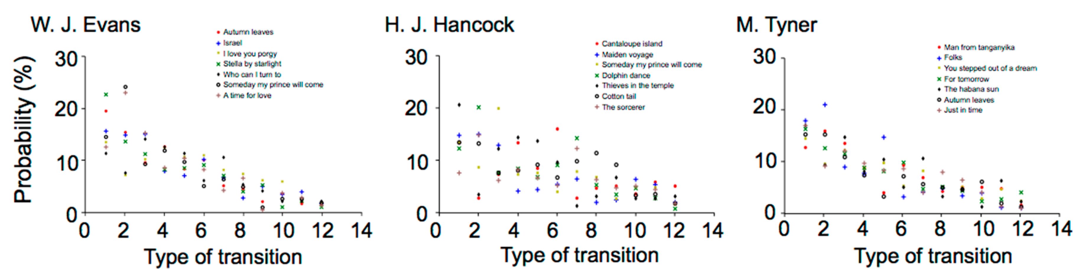
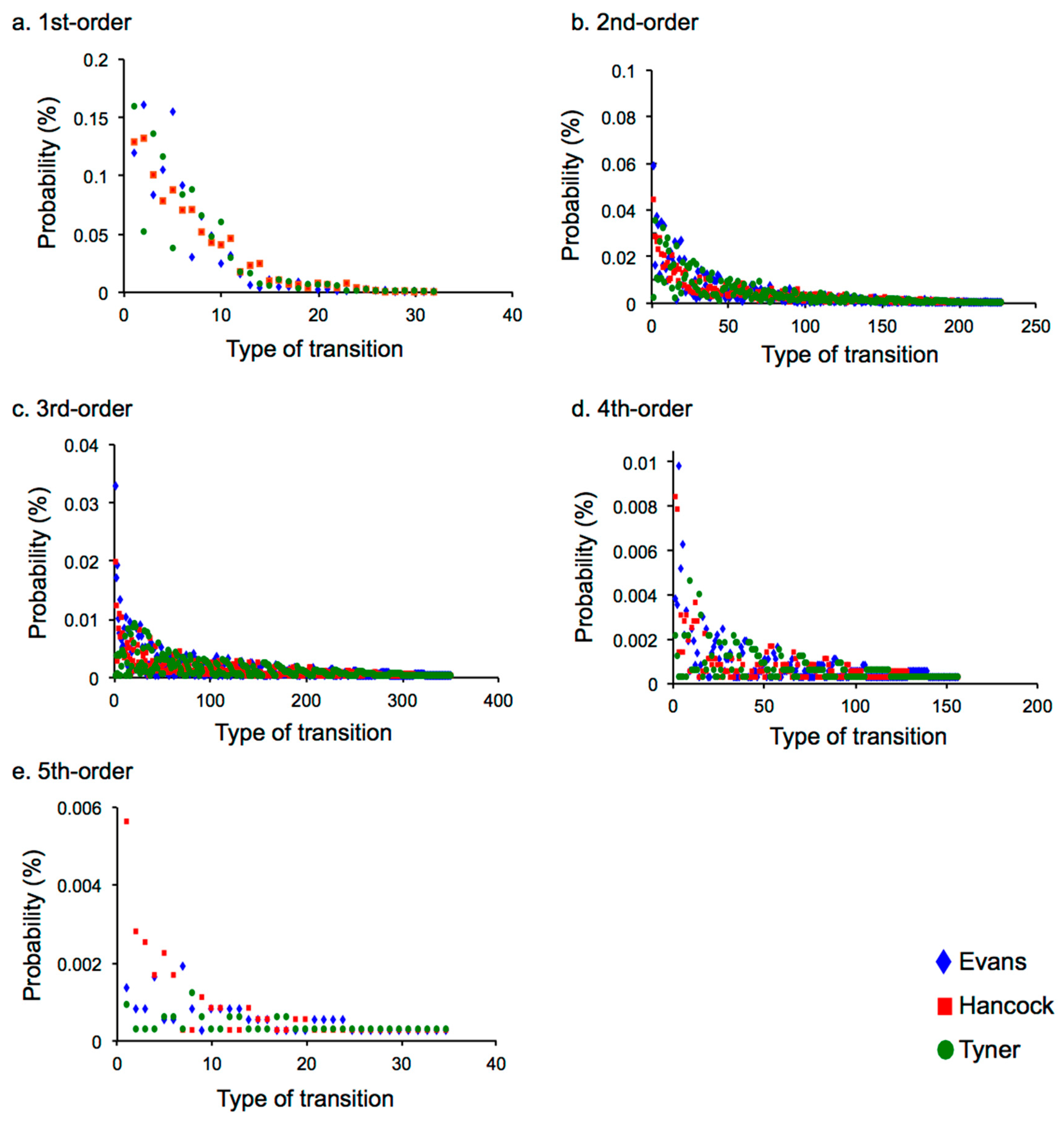
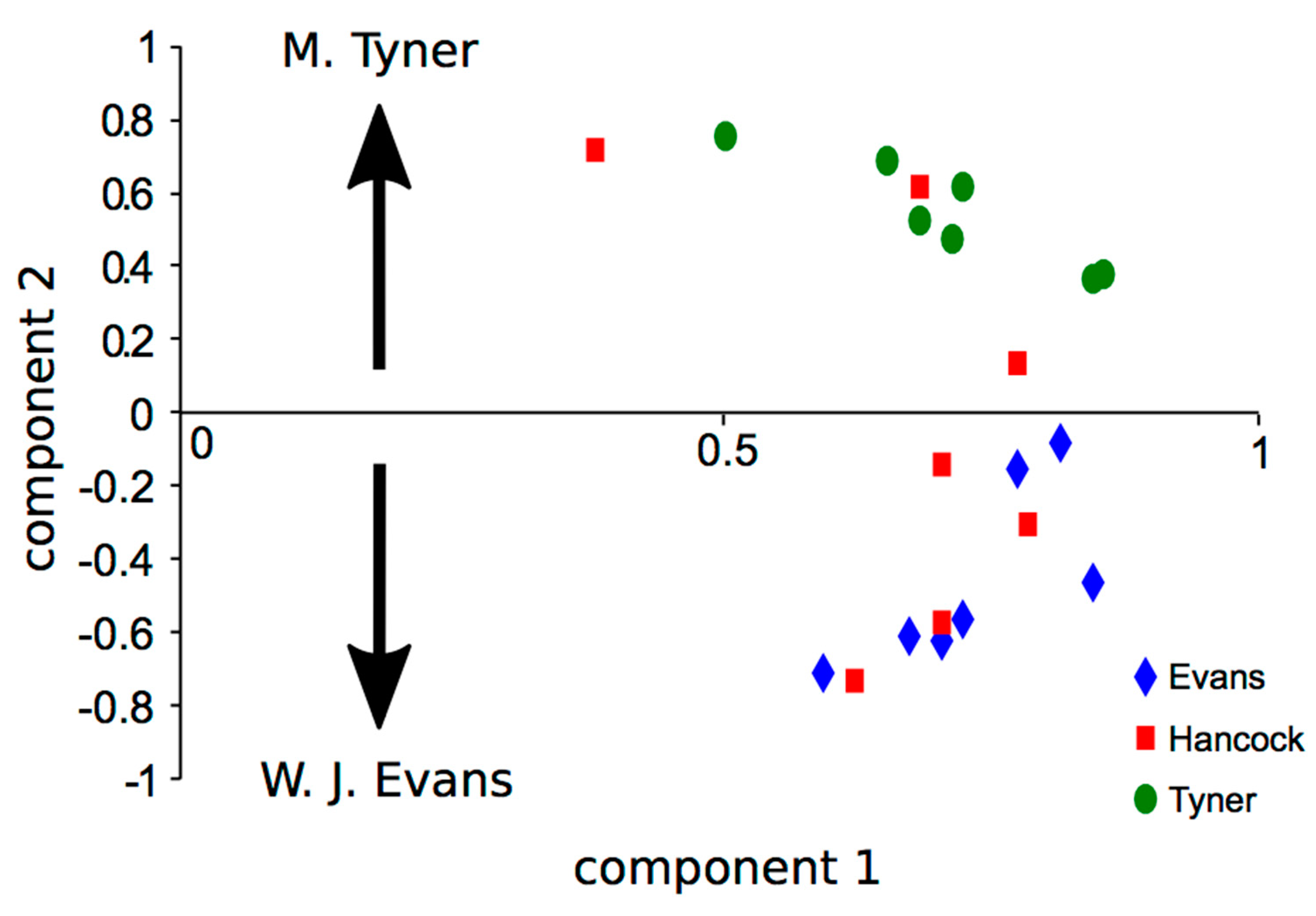
2.2.2. Difference in Statistical Characteristics between Pieces of Music and between Musicians

All of the results in the correlation analysis for each piece of music are shown in the Supplementary Material. All of the pieces of music improvised by W. J. Evans are strongly (0.7 ≦ |r| < 1.0, p < 0.01; Supplementary, red) or moderately (0.4 ≦ |r| < 0.7, p < 0.01; Supplementary, green) related to each other (Figure 3). Some pieces of music improvised by H. J. Hancock and M. Tyner are strongly or moderately related to each other. There were smaller correlations in music improvised by H. J. Hancock than in that by M. Tyner. More correlations between pieces of music improvised by W. J. Evans and H. J. Hancock were detected compared to those between J. Evans and M. Tyner or between H. J. Hancock and M. Tyner.

Correlations could be detected between musicians in the same title of music: between W. J. Evans and M. Tyner in “Autumn Leaves” (r = 0.620), and between W. J. Evans and H. J. Hancock in “Someday My Prince Will Come” (r = 0.719). “Autumn Leaves” improvised by W. J. Evans was related only to “Autumn leaves” improvised by M. Tyner whereas “Autumn Leaves” improvised by M. Tyner was related to six pieces of music improvised by W. J. Evans. All results of the correlation analysis of the weight-averaged TP matrices in each musician are shown in Figure 4. In the first- and second-order TPs, musical improvisations are strongly and moderately related to each other, respectively. In the third-order TP, musical improvisations by H. J. Hancock are weakly (0.2 ≦ |r| < 0.4) related to those by both W. J. Evans (r = 0.356, p < 0.001) and M. Tyner (r = 0.303, p < 0.001). In the fourth- and fifth-order TPs, musical improvisations by W. J. Evans are weakly (r = 0.222, p < 0.001) and moderately (r = 0.409, p < 0.001) related to those by H. J. Hancock, respectively. Musical improvisations by M. Tyner are not, however, related to either those of W. J. Evans or of H. J. Hancock.

In the principal component analysis, the decision was made to specify a four-factor solution (eigenvalue > 1;

Table 3. The results of principal component analysis.

a Eigenvalue, percentages of variance and cumulative variance.
		Total		Variance *	Cumulative *
Component 1		10.79		51.40	51.40		Component 1
Component 2		5.91		28.15	79.55		Component 2
Component 3		1.37		6.52	86.07		Component 3
Component 4		1.21		5.76	91.84		Component 4
b. Eigenvectors for the principal components
			Component 1		Component 2	Component 3		Component 4
W. J. Evans	Autumn leaves		0.71		−0.62	0.09		−0.18
	Israel		0.85		−0.46	−0.12		0.02
	I Love You Porgy		0.78		−0.15	0.34		−0.39
	Stella by Starlight		0.68		−0.61	0.12		−0.16
	Who Can I Turn To		0.82		−0.08	0.52		−0.12
	Some Day My Prince Will Come		0.60		−0.71	0.07		0.19
	A Time for Love		0.73		−0.56	−0.12		0.20
H. J. Hancock	Cantaloupe Island		0.39		0.72	0.24		0.38
	Maiden Voyage		0.71		−0.14	−0.64		0.23
	Some Day My Prince Will Come		0.78		0.14	−0.47		−0.38
	Dolphin Dance		0.71		−0.57	−0.11		0.34
	Thieves in the Temple		0.69		0.62	0.12		0.12
	Cotton Tail		0.79		−0.30	0.21		0.13
	The Sorcerer		0.63		−0.73	0.01		0.15
M. Tyner	Man fromTanganyika		0.72		0.48	−0.06		−0.42
	Folks		0.69		0.53	−0.32		−0.01
	You Stepped Out of a Dream		0.66		0.69	0.03		0.23
	For Tomorrow		0.73		0.62	0.03		−0.03
	The Habana Sun		0.51		0.76	0.03		0.23
	Autumn Leaves		0.85		0.37	−0.13		−0.31
	Just in Time		0.86		0.38	0.20		0.18

* percentage.

and Figure 5). The four factors accounted for 91.84% of the total variance. All of the pieces of music loaded higher than 39 on Factor 1, suggesting that this explains the general component of the jazz musical improvisation of the three musicians. All of the pieces of music improvised by W. J. Evans loaded lower than 0, and those by M. Tyner loaded higher than 0 on Factor 2, suggesting that this explains a component of improvisation in W. J. Evans or M. Tyner. Four pieces of music improvised by H. J. Hancock loaded lower than 0, and the other three pieces of music loaded higher than 0. Factors 3 and 4 did not detect a component for a musician and a piece of music. “Who Can I Turn To?” improvised by W. J. Evans (0.52) and “‘Maiden Voyage” improvised by H. J. Hancock (−0.64) loaded heavily on Factor 3. The representative phrases of transition patterns with the highest probabilities, that were weight-averaged in each musician, were decoded as music scores (Figure 2).

2.3. Discussion

2.3.1. Time-Course Variation of Statistics in Musical Representation

The present study hypothesized that a tone with a higher TP in a musical sequence may be one that a composer is more likely to choose, and that the TP matrix calculated from musical improvisation can represent in part the characteristics of a composer’s statistical knowledge. This study investigated how characteristics of musical improvisation are reflected in TP distributions. Consistent with chronological order in music by W. J. Evans, the third-order TPs of (0,2,3,5] and fourth-order TPs of (0,1,3,4,6] gradually decreased. The third-order TPs of (0,−3,−4,−6] gradually increased. The transition in which TPs gradually decreased (i.e., (0,2,3,5) and (0,1,3,4,6)) may be popular musical phrases compared to the transition in which TPs gradually increased (i.e., (0,−3,−4,−6)). For instance, the transition (0,2,3,5] generally appears as (D,E,F,G] and (A,B,C,D] in C major. The transition (0,1,3,4,6] appears as (C,Db,Eb,E,Gb] in altered scale. This finding suggests that, in the later period of his life, W. J. Evans played statistically novel musical improvisation. In other words, he tried several compositional methods in which he avoided familiar transitional patterns. Consistent with chronological order in the music of M. Tyner, the second-order TPs (0,−2,−5] and (0,5,7] gradually increased and decreased consistently with chronological order, respectively. Both transitions may be popular musical phrases. For instance, the transition (0,−2,−5] appears as (D,C,A], (E,D,B], (G,F,D], and (A,G,E] in C major. In H. J. Hancock, however, no significant time-course variations of TP were detected. From a psychological viewpoint, there might be no chronological variations of statistical knowledge in musical improvisation in H. J. Hancock, compared to W. J. Evans and M. Tyner. These results suggest that time-course (chronological) variations in the statistical knowledge of the composer are reflected in musical improvisation. The time-course variations of statistical structures in musical improvisation may represent those of a composer’s statistical knowledge.

2.3.2. Statistical Characteristics that Depend on Music and Musician

All the pieces of music improvised by W. J. Evans correlated to each other. These findings suggest that there are specific statistical characteristics within music by W. J. Evans. On the other hand, there were smaller correlations in music improvised by H. J. Hancock than by M. Tyner. More correlations between W. J. Evans and H. J. Hancock were detected compared to those between W. J. Evans and M. Tyner or between H. J. Hancock and M. Tyner. In the correlation analysis of the weight-averaged TP matrices for each musician, the lower-order (i.e., first- and second-order) TP distributions are related to each other. On the other hand, in the higher-order (i.e., fourth- and fifth-order) TP distribution, music by W. J. Evans is related to that of H. J. Hancock. Music by M. Tyner is not related to either that of W. J. Evans or of H. J. Hancock. Furthermore, the results of the principal component analysis detected a component of W. J. Evans or M. Tyner but not of H. J. Hancock. Given the chronological order in which musicians played (i.e., W. J. Evans: 1959–1969, H. J. Hancock: 1964–2001), the music by W. J. Evans may have influenced the higher-order statistical knowledge (i.e., knowledge of higher-order transitional probability) of H. J. Hancock when compared to M. Tyner. In other words, at higher-order levels, H. J. Hancock may refer to musical improvisation by W. J. Evans. Correlations could be detected between W. J. Evans and M. Tyner in “Autumn Leaves,” and between W. J. Evans and H. J. Hancock in “Someday My Prince Will Come” (Supplementary Materials). This suggests that there were statistical characteristics of this music shared between different musicians. Furthermore, in W. J. Evans and M. Tyner, “Autumn Leaves” by W. J. Evans was related only to “Autumn Leaves” by M. Tyner whereas “Autumn Leaves” by M. Tyner was related to six pieces of music by W. J. Evans. These results may be logical because of the chronological order. This also supports the hypothesis that H. J. Hancock may refer to musical improvisation by W. J. Evans. The first- to third-order transition patterns with the highest probabilities in H. J. Hancock were also the same as those in W. J. Evans (Figure 2), suggesting the similarity of statistical characteristics between the two musicians.

2.3.3. Improvisation

It is widely accepted that statistical knowledge causes a sense of intuition, spontaneous behaviour and skill acquisition based on procedural learning, and is further closely tied to musical production, including creativity, composition, and playing. Particularly, jazz musicians intuitively engage in musical improvisation based on their knowledge and experience, which do not necessarily follow explicit music-specific rules. They are forced to express intuitive creativity and immediately play their own music based on long-term training associated with procedural and implicit learning. Thus, it is considered that the performance of musical improvisation is intimately bound to statistical knowledge because of the necessity of intuitive decision-making [34,35,36] and auditory-motor planning based on procedural knowledge). That is to say, the statistics embedded in musical improvisation may represent the musician’s individuality of expression that has been developed via learning and knowledge. In the present study, the transitional patterns that appear in all pieces of music were used to verify the statistical characteristics of familiar sequences in musical improvisation. There are several billion types of transitional patterns in music. Thus, it is difficult to define statistical significance when we target all of the transitional patterns. Future study is needed to investigate transitional patterns that do not appear in some pieces of musical improvisation.

It is of note that this study did not directly reveal implicit statistical knowledge of music because only the statistics of musical scores were analyzed. Thus, there may be other possible explanations for the results. For instance, it might be part of a deliberate plan to improvise music moving from familiar to increasingly unfamiliar, based on the statistical structure of music. The possibility cannot be excluded that these findings do not necessarily reflect a composer’s implicit statistical knowledge. Future studies should investigate, in parallel, how implicit statistical learning in music is reflected in neurological response and how learned knowledge is expressed in musical improvisation [27].

3. Study 2

3.1. Methods

The pieces of music were the same as in study 1. We used the improvisational sequences of the highest pitches from 21 pieces of music played by three improvisors (i.e., 7 improvisations per performers, Table 1). The pitches were extracted using the transcriptions by Yasutoshi Inamori (Chuoart Publishing Co., Ltd.), Tomoyuki Hayashi (Doremi Music Publishing Co., Ltd.), The McCoy Tyner Collection: Piano Transcriptions: Jazz Giants (Hal Leonard Corporation), and Herbie Hancock Excellent Performance Collection (Doremi Music Publishing Co., Ltd.). Furthermore, the pitches were also confirmed by hearing. The present study only analyzed the highest pitch because the definition of melody in each musical title is still controversial in musicological study, since different melodies could concurrently appear in different titles of music, and melody is often played at the highest pitches. The highest pitches were chosen based on the following definitions: pitches connected with ties can be counted as one, and grace notes were excluded. Using all the sequences at the highest pitches, TPs were calculated for each piece of music as a statistic based on Markov chains. The nth-order Markov chain is the conditional probability of an event e_n+1, given the preceding n events, based on Bayes’ theorem (see Formula (1)).

Then, for each type of pitch transition, all pitches were numbered so that the first pitch was 0 in each transition, and an increase or decrease in a semitone was 1 and −1 based on the first pitch, respectively. This revealed interval patterns, but not pitch pattern. This procedure was employed to eliminate the effects of change of key on transitional patterns. The interpretation of the change of key depends on the musician, and it is difficult to define in an objective manner. Thus, the results in the present study may represent a variation of the statistics associated with relative pitch rather than absolute pitch. Only the transitional patterns that appear in all music were used in the present study (

Table 4. The transitional patterns of pitch intervals that appear in all music sequences based on 0th- and first-order Markov models.

0th-Order	1st-Order
0	2,0
1	−2,0
−1	2,4
2	−2,−4
−2	−2,−5
3	−2,−7
−3	3,0
4	−3,−5
−4	3,7
5	−4,−7
−5	5,3
7

). From the second-order Markov chains of interval transitions, transitional patterns that appear in all music could not be detected. Information content (I) was calculated using TPs in the framework of information theory.

I(P(e_n+1|e_n)) = log₂ 1/P(e_n+1|e_n) (bit)

(2)

Chi-square-test for uniformity (goodness-of-fit test) was conducted to analyze TP distributions, followed by repeated-measure analysis of variances (ANOVAs) with a between-factor improviser (Bill Evans vs Herbie Hancock vs McCoy Tyner), and a within-factor sequences for each hierarchy of the Markov model (i.e., 0th- and first-order Markov chains). When significant effects were detected, Bonferroni-corrected post-hoc tests were conducted for further analysis. Statistical significance levels were set at p < 0.05 for all analyses.

3.2. Results

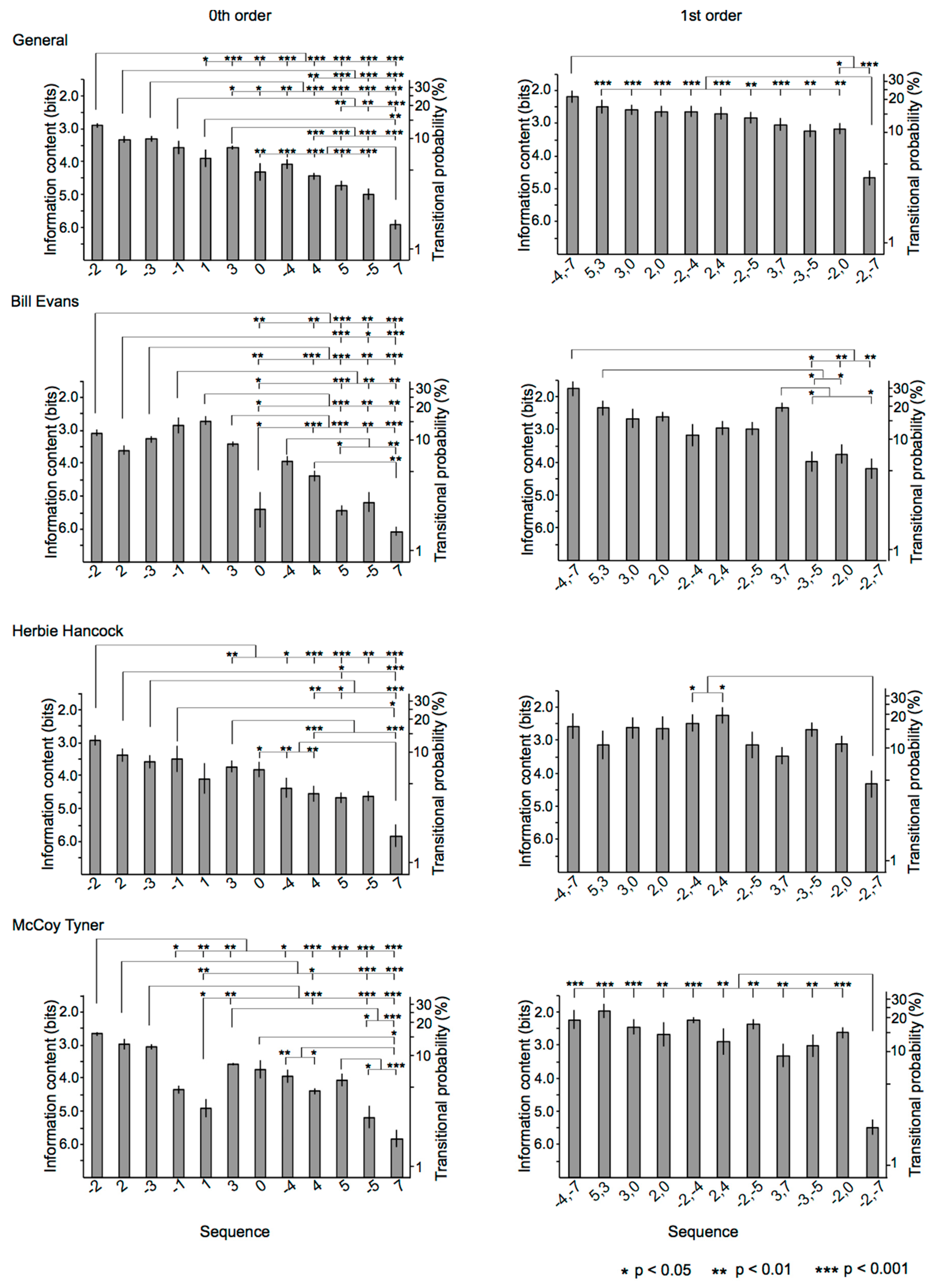
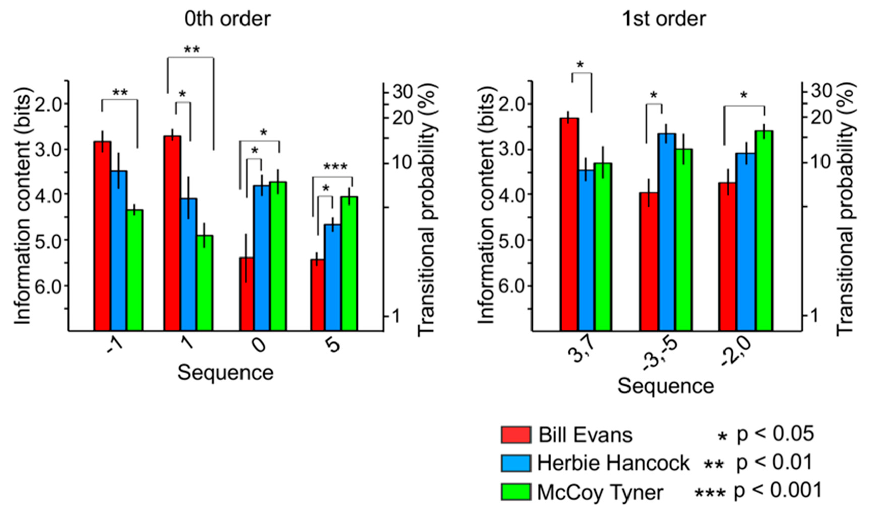
3.2.1. 0th-Order Markov Model

The main sequence effect was significant (F (4.25, 76.50) = 32.38, p < 0.001, partialη² = 0.64) (Figure 6). The TPs of (−2) were significantly higher than those of (1) (p = 0.044), (3) (p < 0.001), (0) (p = 0.001), (−4) (p < 0.001), (4) (p < 0.001), (5) (p < 0.001), (−5) (p < 0.001), and (7) (p < 0.001). The TPs of (2) were significantly higher than those of (4) (p = 0.001), (5) (p < 0.001), (−5) (p < 0.001), and (7) (p < 0.001). The TPs of (−3) were significantly higher than those of (3) (p = 0.017), (0) (p = 0.026), (−4) (p = 0.003), and (4) (p < 0.001), (5) (p < 0.001), (−5) (p < 0.001), and (7) (p < 0.001). The TPs of (−1) were significantly higher than those of (5) (p = 0.002), (−5) (p = 0.001), and (7) (p < 0.001). The TPs of (1) were significantly higher than those of (7) (p = 0.001). The TPs of (3) were significantly higher than those of (4), (5), (−5), and (7) (all: p < 0.001). The TPs of (7) were significantly lower than those of (0) (p = 0.001), (−4) (p < 0.001), (4) (p < 0.001), (5) (p < 0.001), and (−5) (p < 0.001).

The improviser-sequence interactions were significant (F (22) = 2.28, p < 0.001, partialη² = 0.35) (Figure 6). In Bill Evans, the TPs of (−2) were significantly higher than those of (0) (p = 0.001), (4) (p = 0.002), (5) (p < 0.001), (−5) (p = 0.001), and (7) (p < 0.001). The TPs of (2) were significantly higher than those of (5) (p < 0.001), (−5) (p = 0.021) and (7) (p < 0.001). The TPs of (−3) were significantly higher than those of (0) (p = 0.003), (4) (p < 0.001), (5) (p < 0.001), (−5) (p = 0.001), and (7) (p < 0.001). The TPs of (−1) were significantly higher than those of (0) (p = 0.043), (5) (p < 0.001), (−5) (p = 0.002), and (7) (p = 0.001). The TPs of (1) were significantly higher than those of (0) (p = 0.015), (5) (p < 0.001), (−5) (p = 0.003), and (7) (p = 0.001). The TPs of (3) were significantly higher than those of (0) (p = 0.010), (4) (p < 0.001), (5) (p < 0.001), (−5) (p = 0.005), and (7) (p < 0.001). The TPs of (−4) were significantly higher than those of (5) (p = 0.011) and (7) (p = 0.001). The TPs of (4) were significantly higher than those of (7) (p = 0.002).

In Herbie Hancock, the TPs of (−2) were significantly higher than those of (3) (p = 0.003), (−4) (p = 0.012), (4) (p < 0.001), (5) (p < 0.001), (−5) (p = 0.008), and (7) (p < 0.001). The TPs of (2) were significantly higher than those of (5) (p = 0.011) and (7) (p < 0.001). The TPs of (−3) were significantly higher than those of (4) (p = 0.001), (5) (p = 0.031), and (7) (p < 0.001). The TPs of (−1) were significantly higher than those of (7) (p = 0.022). The TPs of (3) were significantly higher than those of (4) (p < 0.001) and (7) (p < 0.001). The TPs of (7) were significantly lower than those of (0) (p = 0.019), (−4) (p = 0.001), and (4) (p = 0.002).

In McCoy Tyner, the TPs of (−2) were significantly higher than those of (−1) (p = 0.014), (1) (p = 0.003), (3) (p = 0.001), (−4) (p = 0.042), and (4), (5), (−5), and (7) (all: p < 0.001). The TPs of (2) were significantly higher than those of (1) (p = 0.006), (4) (p = 0.032), (−5) (p < 0.001), and (7) (p < 0.001). The TPs of (−3) were significantly higher than those of (1) (p = 0.044), (3) (p = 0.009), (4) (p < 0.001), (−5) (p < 0.001), and (7) (p < 0.001). The TPs of (3) were significantly higher than those of (−5) (p = 0.013) and (7) (p < 0.001). The TPs of (0) were significantly higher than those of (7) (p = 0.013). The TPs of (−4) were significantly higher than those of (7) (p = 0.005). The TPs of (4) were significantly higher than those of (7) (p = 0.011). The TPs of (5) were significantly higher than those of (−5) (p = 0.019) and (7) (p < 0.001).

In the sequence of (−1), the TPs in Bill Evans were significantly higher than those in McCoy Tyner (p = 0.009) (Figure 7). In the sequence of (1), the TPs in Bill Evans were significantly higher than those in Herbie Hancock (p = 0.033) and McCoy Tyner (p = 0.001). In the sequence of (0), the TPs in Bill Evans were significantly lower than those in Herbie Hancock (p = 0.036) and McCoy Tyner (p = 0.028). In the sequence of (5), the TPs in Bill Evans were significantly lower than those in Herbie Hancock (p = 0.023) and McCoy Tyner (p < 0.001).

3.2.2. First-Order Markov Model

The main sequence effect was significant (F (6.43, 115.67) = 13.40, p < 00.001, partialη² = 0.43) (Figure 6). The TPs of (−4,−7) were significantly higher than those of (−2,0) (p = 0.019) and (−2,−7) (p < 0.001). The TPs of (−2,−7) were significantly lower than those of (5,3) (p < 0.001), (3,0) (p < 0.001), (2,0) (p < 0.001), (−2,−4) (p < 0.001), (2,4) (p < 0.001), (−2,−5) (p = 0.001), (3,7) (p < 0.001), (−3,−5) (p = 0.004), and (−2,0) (p = 0.001).

The improviser-sequence interactions were significant (F (20) = 2.83, p < 00.001, partialη² = 0.24) (Figure 6). In Bill Evans, the TPs of (−4,−7) were significantly higher than those of (−3,−5) (p = 0.024), (−2,0) (p = 0.004) and (−2,−7) (p = 0.009). The TPs of (5,3) were significantly higher than those of (−3,−5) (p = 0.031) and (−2,0) (p = 0.021). The TPs of (3,7) were significantly higher than those of (−3,−5) (p = 0.020) and (−2,−7) (p = 0.013). In Herbie Hancock, the TPs of (−2,−7) were significantly lower than those of (−2,−4) (p = 0.047) and (2,4) (p = 0.016). In McCoy Tyner, the TPs of (−2,−7) were significantly lower than those of (−4,−7) (p < 0.001), (5,3) (p < 0.001), (3,0) (p < 0.001), (2,0) (p = 0.001), (−2,−4) (p < 0.001), (2,4) (p = 0.002), (−2,−5) (p = 0.002), (3,7) (p = 0.003), (−3,−5) (p = 0.005), (−2,0) (p < 0.001).

In the sequence of (3,7), the TPs in Bill Evans were significantly higher than those in Herbie Hancock (p = 0.034) (Figure 7). In the sequence of (−3,−5), the TPs in Bill Evans were significantly lower than those in Herbie Hancock (p = 0.034). In the sequence of (−2,0), the TPs in Bill Evans were significantly lower than those in McCoy Tyner (p = 0.023).

3.3. Discussion

3.3.1. Relationships among Sequences

The present study examined the statistical structure embedded in musical improvisation based on various-order hierarchical models of TPs to reveal the statistical differences among improvisers. The TPs of the improvisational sequences containing the highest pitches in the pieces of music played by Bill Evans, McCoy Tyner, and Herbie Hancock were calculated based on different hierarchical Markov stochastic models. The TPs were compared among improvisers and sequences. It was hypothesized that there were general statistical characteristics shared among jazz improvisers, and specific statistical characteristics unique to each improviser. If so, statistical similarity may represent common styles all improvisers shared, whereas statistical differences among improvisers may represent the specific characteristics of each improviser. Thus, universal and independent statistical knowledge among improvisers can be disclosed by computational analysis of music based on the Markov model of pitch intervals in the framework of statistical learning.

In the 0th-order Markov model, the smaller the pitch interval, the higher the TP (Figure 6). From a psychological perspective, statistical learning of TPs contributes to chunk perception. For example, humans can recognize pattern and phrase embedded in tone sequences by calculating the TPs of the sequences, because TPs within phrases are higher than those between phrases. Thus, the present findings may suggest that smaller intervals of pitch can be perceived as a phrase. Furthermore, the findings in the first-order hierarchical model may also support the hypothesis that statistical learning contributes to musical improvisation. In this model, sequences that consisted of intervals of major and minor thirds (i.e., (−4,−7)), which produce a minor chord, showed the highest TPs. These sequences are also frequently used in music. On the other hand, other studies also claim that the perception of music is associated with the gestalt principle [28]. Generally, a sequence in which the interval between adjacent tones is not large is likely to be perceived as a phrase in the framework of the gestalt principle. Thus, the present findings may reflect gestalt perception as well as statistical learning. Future study is needed to investigate how these interact with each other in music perception and production using a number of pieces of improvisational music.

3.3.2. Relationships among Improvisers

The TP of the sequence of (−1) and (1) was lower in McCoy Tyner than in Bill Evans and Herbie Hancock (Figure 7). In contrast, the TP of the sequence of (0), (5), and (−2,0) showed opposite trends. The TPs of these sequences were higher in McCoy Tyner than in Bill Evans and Herbie Hancock. Difference could also be detected between Bill Evans and Herbie Hancock (i.e., (1), (3,7), and (−3,−5)). These results may support the hypothesis that musical improvisation partially depends on statistical knowledge. The individuality of improvisation style may be reflected in TP distribution in music. Interestingly, the results detected general trends of TPs among the three improvisers. The largest difference in TPs was between Bill Evans and McCoy Tyner, and the TPs in Herbie Hancock took a middle position between those of Bill Evans and McCoy Tyner. It would be interesting to determine if these trends among three improvisers represent how the musical improvisations of an improviser influence those by another improviser in the context of statistical knowledge.

3.3.3. Statistical Learning in Psychological and Computational Studies

To understand the brain’s higher-order statistical learning systems in a form closer to that used for music, sequential paradigms based on higher-order Markov models have been used in neurophysiological [6,8] as well as computational studies [19]. Furthermore, the nth-order Markov model has been applied to develop artificial intelligence that gives computers learning and decision-making abilities similar to those of the human brain, thus generating systems for automatic music composition [17,42,43]. Such models can verify hierarchies of statistical learning based on various-order TPs. Music includes higher-order statistics such as hierarchical syntactical structures and grammar. Thus, information-theoretical approaches, including information content based on nth-order Markov models, may be useful in understanding the SL as it functions in response to real-world learning phenomena in the interdisciplinary realms of brain and computational sciences.

Recent neural studies have suggested that, during statistical learning, the brain codes the statistics of auditory sequences as relative information, such as relative distribution of pitch frequencies, and that this information can be used in the comprehension of other sequential structures [7]. This suggests that the brain does not have to code and accumulate all received information and thus saves some memory capacity [44]. Thus, from the perspective of information theory [18], the brain’s SL is systematically efficient. Based on these neural findings, the present computational study investigated TP distributions of relative pitches (i.e., pitch interval) in musical improvisation. The results support the hypothesis that specific as well as general characteristics among improvisers can be detected in TP distributions of pitch intervals. These results may suggest that statistical similarities and differences represent common and specific styles among improvisers, and that universal and independent statistical knowledge among improvisers can be disclosed by computational analysis of music based on the Markov model of pitch intervals in the framework of statistical learning. It is of note, however, that the present study did not directly investigate the musicians’ statistical knowledge of music, as only the statistics of musical scores were analyzed. This suggests that there may be other possible explanations for its findings. For instance, it might have been the musician’s plan to engage in improvisation that is statistically different from other specific music. Moreover, it is not clear if actual probabilities are learned regardless of domain-specific features of music such as tonalities and harmonic syntax. Indeed, these three jazz masters may have very distinct personal styles, and are generally regarded as among the more influential jazz pianists.

Transition probabilities, however, shape only a small part of their respective styles. The neural correlates of such computational models have been investigated by a body of previous studies (see review, [45,46]. For example, the n-gram model, which is frequently verified by neural approaches, is considered to correspond to chunking and word-segmentation processes in statistical learning [2]. The online perception and production of music, however, is not the mere chunking of sequential patterns, like word segmentation, but is a dynamic form of prediction to maintain an aesthetic melody with various temporal and spectral features [47], hierarchical building, and harmonics [48], which interact with each other [28]. Musical prediction and representation are not restricted to a single stream of events but, rather, they interact with each parallel stream [49,50,51]. However, future study is needed to investigate other aspects of music such as harmony and the hierarchical building of not only single but parallel streams forming harmony.

4. Conclusions

The present study investigated how statistical knowledge is reflected in musical improvisation by analyzing statistical structures in music and differences between musicians and between pieces of music. First, the results suggest that time-course variations of statistical structures in music may represent time-course variations of a musician’s statistical knowledge, by which a forthcoming tone is statistically defined. Second, the results suggest that there are specific statistical characteristics shared between distinct pieces of music of the same title played by different musicians and between pieces of music of distinct titles played by the same musician. Third, the musical improvisation of a musician may influence the higher-order statistical knowledge (i.e., knowledge of higher-order transitional probability) of other musicians without explicit intention and awareness. Fourth, the results showed the statistical similarities and differences of improvisers’ individuality. The present study sheds new light on novel methodologies that can be employed to evaluate how musical improvisations are influenced by other musical improvisations via statistical learning, using interdisciplinary approaches including Psychology, Musicology, and Informatics.

References

1. Perruchet, P.; Pacton, S. Implicit learning and statistical learning: one phenomenon, two approaches. Trends Cogn. Sci. 2006, 10, 233–238. [Google Scholar] [CrossRef] [PubMed]
2. Saffran, J.R.; Aslin, R.N.; Newport, E.L. Statistical learning by 8-month-old infants. Science 1996, 274, 1926–1928. [Google Scholar] [CrossRef] [PubMed] [Green Version]
3. Cleeremans, A.; Destrebecqz, A.; Boyer, M. Implicit learning: News from the front. Trends Cogn. Sci. 1998, 2, 406–416. [Google Scholar] [CrossRef]
4. Teinonen, T.; Fellman, V.; Näätänen, R.; Alku, P.; Huotilainen, M. Statistical language learning in neonates revealed by event-related brain potentials. BMC Neurosci. 2009, 10. [Google Scholar] [CrossRef] [PubMed] [Green Version]
5. Kudo, N.; Nonaka, Y.; Mizuno, N.; Mizuno, K.; Okanoya, K. On-line statistical segmentation of a non-speech auditory stream in neonates as demonstrated by event-related brain potentials. Dev. Sci. 2011, 5, 1100–1106. [Google Scholar] [CrossRef] [PubMed]
6. Furl, N.; Kumar, S.; Alter, K.; Durrant, S.; Shawe-Taylor, J.; Griffiths, T.D. Neural prediction of higher-order auditory sequence statistics. NeuroImage 2011, 54, 2267–2277. [Google Scholar] [CrossRef] [PubMed]
7. Daikoku, T.; Yatomi, Y.; Yumoto, M. Statistical learning of music- and language-like sequences and tolerance for spectral shifts. Neurobiol. Learn. Mem. 2015, 118, 8–19. [Google Scholar] [CrossRef] [Green Version]
8. Daikoku, T.; Yatomi, Y.; Yumoto, M. Implicit and explicit statistical learning of tone sequences across spectral shifts. Neuropsychologia 2014, 63. [Google Scholar] [CrossRef] [Green Version]
9. Daikoku, T.; Yatomi, Y.; Yumoto, M. Pitch-class distribution modulates the statistical learning of atonal chord sequences. Brain Cogn. 2016, 108. [Google Scholar] [CrossRef] [Green Version]
10. Daikoku, T.; Yumoto, M. Single, but not dual, attention facilitates statistical learning of two concurrent auditory sequences. Sci. Rep. 2017, 7. [Google Scholar] [CrossRef]
11. Daikoku, T.; Yumoto, M. Concurrent statistical learning of ignored and attended sound sequences: An MEG study. Front. Hum. Neurosci. 2019. [Google Scholar] [CrossRef] [PubMed] [Green Version]
12. Daikoku, T.; Yatomi, Y.; Yumoto, M. Statistical learning of an auditory sequence and reorganization of acquired knowledge: A time course of word segmentation and ordering. Neuropsychologia 2017, 95, 1–10. [Google Scholar] [CrossRef] [PubMed]
13. Koelsch, S.; Busch, T.; Jentschke, S.; Rohrmeier, M. Under the hood of statistical learning: A statistical MMN reflects the magnitude of transitional probabilities in auditory sequences. Sci. Rep. 2016, 6, 1–11. [Google Scholar] [CrossRef] [PubMed] [Green Version]
14. Daikoku, T. Tonality Tunes the Statistical Characteristics in Music: Computational Approaches on Statistical Learning. Front. Comput. Neurosci. 2019, 13, 70. [Google Scholar] [CrossRef]
15. Daikoku, T. Statistical learning and the uncertainty of melody and bass line in music. PLoS ONE 2019, 14, e0226734. [Google Scholar] [CrossRef]
16. Daikoku, T. Time-course variation of statistics embedded in music: Corpus study on implicit learning and knowledge. PLoS ONE 2018, 13, e0196493. [Google Scholar] [CrossRef] [Green Version]
17. Boenn, G.; Brain, M.; De Vos, M.; Ffitch, J. Automatic Composition of Melodic and Harmonic Music by Answer Set Programming BT. In Logic Programming; Garcia de la Banda, M., Pontelli, E., Eds.; Springer: Heidelberg, German, 2008; pp. 160–174. [Google Scholar]
18. Shannon, C.E. A Mathematical Theory of Communication. Bell Syst. Tech. J. 1948, 27, 623–656. [Google Scholar] [CrossRef]
19. Pearce, M.T.; Wiggins, G.A. Auditory Expectation: The Information Dynamics of Music Perception and Cognition. Top. Cogn. Sci. 2012, 4, 625–652. [Google Scholar] [CrossRef]
20. Pearce, M.; Wiggins, G. Expectation in melody: The Influence of Context and Learning. Music Percept. 2006, 23, 377–405. [Google Scholar] [CrossRef] [Green Version]
21. Pearce, M.T.; Ruiz, M.H.; Kapasi, S.; Wiggins, G.A.; Bhattacharya, J. Unsupervised statistical learning underpins computational, behavioural, and neural manifestations of musical expectation. NeuroImage 2010, 50, 302–313. [Google Scholar] [CrossRef]
22. Omigie, D.; Pearce, M.T.; Stewart, L. Tracking of pitch probabilities in congenital amusia. Neuropsychologia 2012, 50, 1483–1493. [Google Scholar] [CrossRef] [PubMed]
23. Hansen, N.C.; Pearce, M.T. Predictive uncertainty in auditory sequence processing. Front. Psychol. 2014, 5, 1–17. [Google Scholar] [CrossRef] [PubMed] [Green Version]
24. Daikoku, T. Depth and the Uncertainty of Statistical Knowledge on Musical Creativity Fluctuate Over a Composer’s Lifetime. Front. Comput. Neurosci. 2019, 13, 27. [Google Scholar] [PubMed]
25. Daikoku, T. Method and Apparatus for Analyzing Characteristics of Music Information. U.S. Patent US20190189100, 1 October 2019. [Google Scholar]
26. Daikoku, T. Implicit learning in the developing brain: An exploration of ERP indices for developmental disorders. Clin. Neurophysiol. 2019, 130, 2166–2168. [Google Scholar] [CrossRef] [PubMed]
27. Daikoku, T. Computational models and neural bases of statistical learning in music and language: Comment on “Creativity, information, and consciousness: The information dynamics of thinking” by Wiggins. Phys. Life. Rev. 2019. [Google Scholar] [CrossRef]
28. Jackendoff, R.; Lerdahl, F. The capacity for music: What is it, and what’s special about it? Cognition 2006, 100, 33–72. [Google Scholar] [CrossRef]
29. Hauser, M.D.; Chomsky, N.; Fitch, W.T. The Faculty of Language: What Is It, Who Has It, and How Did It Evolve? Science 2002, 298, 1569 LP-1579. [Google Scholar] [CrossRef]
30. Clark, R.E.; Squire, L.R. Classical Conditioning and Brain Systems: The Role of Awareness. Science 1998, 280, 77–81. [Google Scholar] [CrossRef]
31. De Jong, N. Learning Second Language Grammar by Listening. Ph.D. Thesis, Netherlands Graduate School of Linguistics, Amsterdam, The Netherlands, 2005. [Google Scholar] [CrossRef]
32. Ellis, R. Implicitand Explicit Learning, Knowledge and Instruction. In Implicit and Explicit Knowledge in Second Language Learning, Testing and Teaching; Ellis, R., Loewen, S., Elder, C., Erlam, R., Philip, J., Reinders, H., Eds.; Multilingual Matters: Bristol, UK, 2009; pp. 3–25. [Google Scholar] [CrossRef]
33. Paradis, M. A Neurolinguistic Theory of Bilingualism; John Benjamins: Amsterdam, The Netherlands, 2004. [Google Scholar]
34. Berry, D.; Dienes, Z. Implicit Learning: Theoretical and Empirical Issues; Lawrence Erlbaum: Hove, UK, 1993. [Google Scholar]
35. Reber, A.S. Implicit Learning and Tacit Knowledge: An Essay on the Cognitive Unconscious; Oxford University Press: Oxford, UK, 1993. [Google Scholar]
36. Perkovic, S.; Orquin, J.L. Implicit Statistical Learning in Real-World Environments Leads to Ecologically Rational Decision Making. Psychol. Sci. 2017, 29, 34–44. [Google Scholar] [CrossRef]
37. Egermann, H.; Pearce, M.T.; Wiggins, G.A.; McAdams, S. Probabilistic models of expectation violation predict psychophysiological emotional responses to live concert music. Cogn. Affect. Behav. Neurosci. 2013, 13, 533–553. [Google Scholar] [CrossRef] [Green Version]
38. Pearce, M.T.; Müllensiefen, D.; Wiggins, G.A. The Role of Expectation and Probabilistic Learning in Auditory Boundary Perception: A Model Comparison. Perception 2010, 39, 1367–1391. [Google Scholar] [CrossRef] [PubMed] [Green Version]
39. Zioga, I.; Harrison, P.M.C.; Pearce, M.T.; Bhattacharya, J.; Di Bernardi Luft, C. From learning to creativity: Identifying the behavioural and neural correlates of learning to predict human judgements of musical creativity. NeuroImage 2019, 206, 116311. [Google Scholar] [CrossRef] [PubMed]
40. Daikoku, T. Entropy, Uncertainty, and the Depth of Implicit Knowledge on Musical Creativity: Computational Study of Improvisation in Melody and Rhythm. Front. Comput. Neurosci. 2018, 12, 1–11. [Google Scholar] [CrossRef] [PubMed] [Green Version]
41. Daikoku, T. Musical Creativity and Depth of Implicit Knowledge: Spectral and Temporal Individualities in Improvisation. Front Comput. Neurosci. 2018, 12, 1–27. [Google Scholar] [CrossRef] [PubMed]
42. Raphael, C.; Stoddard, J. Functional Harmonic Analysis Using Probabilistic Models. Comput. Music J. 2004, 28, 45–52. [Google Scholar] [CrossRef]
43. Eigenfield, A.; Pasquier, P. Realtime Generation of Harmonic Progressions Using Controlled Markov Selection. Available online: http://metacreation.net/wp-content/uploads/2014/09/Controlled_Markov_Selection_2010.pdf (accessed on 20 September 2020).
44. Olshausen, B.A.; Field, D.J. Sparse coding of sensory inputs. Curr. Opin. Neurobiol. 2004, 14, 481–487. [Google Scholar] [CrossRef] [PubMed]
45. Daikoku, T. Neurophysiological markers of statistical learning in music and language: Hierarchy, entropy, and uncertainty. Brain Sci. 2018, 8, 114. [Google Scholar] [CrossRef] [Green Version]
46. Yumoto, M.; Daikoku, T. Neurophysiological Studies on Auditory Statistical Learning (in Japanese). Jpn. J. Cogn. Neurosci. 2018, 20, 38–43. [Google Scholar]
47. Daikoku, T.; Yumoto, M. Musical Expertise Facilitates Statistical Learning of Rhythm and the Perceptive Uncertainty: A cross-cultural Study. Neuropsychologia 2020, 146, 107553. [Google Scholar] [CrossRef]
48. Daikoku, T.; Ogura, H.; Watanabe, M. The variation of hemodynamics relative to listening to consonance or dissonance during chord progression. Neurological Res. 2012, 34, 557–563. [Google Scholar] [CrossRef]
49. Conklin, D.; Witten, I.H. Multiple viewpoint systems for music prediction. J. New Music. Res. 1995, 24, 51–73. [Google Scholar] [CrossRef]
50. Daikoku, T.; Takahashi, Y.; Futagami, H.; Tarumoto, M.; Yasuda, H. Physical fitness modulates incidental but not intentional statistical learning of simultaneous auditory sequences during concurrent physical exercise. Neurol. Res. 2017, 30, 107–116. [Google Scholar] [CrossRef] [PubMed]
51. Daikoku, T.; Takahashi, Y.; Tarumoto, M.; Yasuda, H. Auditory Statistical Learning During Concurrent Physical Exercise and the Tolerance for Pitch, Tempo, and Rhythm Changes. Motor Control 2018, 22, 233–244. [Google Scholar] [CrossRef] [PubMed]
Figure 1. Example of transitional probability (TP) matrices based on nth-order Markov models calculated from a sequence.
Neurosci 01 00004 g001
Figure 2. Representative phrases of transition patterns with the highest probabilities that were weight-averaged in the five different hierarchical models of TPs in each musician.
Neurosci 01 00004 g002
Figure 3. TPs in transition patterns in each piece of music by W. J. Evans, H. J. Hancock, and M. Tyner. The horizontal and vertical axes represent the types of transition and the TPs, respectively. The transition patterns are arranged in descending order of TPs.
Neurosci 01 00004 g003
Figure 4. Weight-averaged TPs in transition patterns in music by W. J. Evans, H. J. Hancock, and M. Tyner. The horizontal and vertical axes represent the types of transition and the TPs, respectively. The transition patterns are arranged in the descending order of TPs.
Neurosci 01 00004 g004
Figure 5. Principal component analysis scatter plots. The horizontal and vertical axes represent principal component 1 and 2, respectively. The dots represent each piece of music.
Neurosci 01 00004 g005
Figure 6. Difference in TPs among sequences based on the 0th- and first-order Markov chains in Bill Evans, Herbie Hancock, and McCoy Tyner.
Neurosci 01 00004 g006
Figure 7. Difference in TPs among Bill Evans (red), Herbie Hancock (blue), and McCoy Tyner (green) in sequences based on the 0th- (left) and first-order (right) Markov chains.
Neurosci 01 00004 g007