Similarity and Homogeneity of Climate Change in Local Destinations: A Globally Reproducible Approach from Slovakia

Abstract

In terms of climate change, while tourism’s natural resources may be considered climate vulnerable, a large part of tourism’s primary industries are high carbon consumers. With the growth of worldwide efforts to adopt climate resilience actions across all industries, Destination Management Organizations could become focal points for raising awareness and leadership among local tourism stakeholders. The manuscript communicates a simple, reproducible approach to observing and analyzing climate change at a high territorial granularity to empower local destinations with the capability to disseminate quantifiable information about past, current, and future climate projections. In relation to Slovakia’s 39 local destinations, the approach utilizes six sub-sets of the latest high-resolution Köppen–Geiger climate classification grid data. The main climate categories’ similarity for local destinations was measured across six periods through the Pearson Correlation Coefficient of Pairwise Euclidean Distances between the linkage matrices of hierarchical clusters adopting Ward’s Linkage Method. The Shannon Entropy Analysis was adopted for the quantification of the homogeneity of the DMOs’ main climate categories, and Weighted Variance Analysis was adopted to identify the main climate categories’ weight fluctuations. The current results indicate not only a major shift from destination climates classified as cold to temperate, but also a transformation to more heterogeneous climates in the future.

1. Introduction

To date, the more than a decade old Paris Agreement, recognizing the necessity of systematic change in several domains of humankind’s existence in relation to the Earth’s environment, has been signed by 194 countries and the European Union (United Nations, 2015) [1]. The urgent necessity of adopting systematic measures in tourism, concerning the climate crisis, has also been recognized globally. In collaboration with United Nations (UN) agencies, over 850 organizations worldwide, as signatories of the Glasgow Declaration, agreed upon five common approaches to tackling the current and future threats of climate change in tourism (One Planet Sustainable Tourism Programme, 2021) [2]. In support of the Glasgow Declaration, the World Tourism Organization (UNWTO) has not only recognized the threats of climate change to tourism, but also acknowledged tourism’s negative impact, as it is responsible for 8–10% of global greenhouse gas emissions (GHG emissions), and most importantly created policy guidance for National Tourism Administrators (NTAs) to adopt systematic climate actions (UNWTO, 2024) [3]. The European Union (EU) also recognizes the tourism industry’s responsibility for GHG emissions and related consequences; therefore, the EU integrated several climate change-related actions in its “European Agenda for Tourism 2030” framework (Council of the European Union, 2022) [4]. All three of the frameworks highlight the necessity of raising awareness among tourists and stakeholders through digital tools, monitoring, and data collection on the industry’s environmental and socioeconomic impacts; all-level cooperation among stakeholders; and of allocating funding for local actions.

As the urgency of climate action increases, particularly at a global scale, there is increasing recognition of the critical role that Destination Management Organizations (DMOs) can play in local adaptation and mitigation strategies. The manuscript responds to that call by communicating a reproducible and data-driven approach to assessing climate change impacts at a granular level, specifically targeting local DMOs in Slovakia. Utilizing high-resolution Köppen–Geiger climate classification datasets and spatiotemporal statistical techniques, the case provides a transparent, scalable framework that can be adopted by DMOs globally. The study aims not only to reveal patterns of climatic transformation but also to empower DMOs with accessible tools for raising awareness, guiding policy, and enhancing destination resilience.

2. Literature Review

Since the climate shapes a destination’s natural environment, and thus its primary resources, it should be considered one of the essential prerequisites for both tourism development and sustainability. Concerns about climate change’s impact on tourism and vice versa have been a focal point of several case studies and global research efforts focusing on different partial aspects of the domain.

2.1. DMOs and Climate Change

The essential role of DMOs in local tourism adaptation and transition has been recognized over recent years. Scott et al. (2008) clearly defined the criticality of tourism industries’ and local destinations’ adaptation to climate change [5].

Dodds (2010) interviewed Canadian DMOs and identified that, due to a lack of proper technologies, accessibility, and finance, DMOs are subjectively not able to take on the role of climate change educators for local tourism stakeholders and as leaders in the fostering of preparedness in tourism-related climate change [6]. Bhandari et al. (2014) pointed out DMOs’ key role in learning and disseminating climate science among local stakeholders and further designated them as knowledge integrators for developing climate-informed strategies [7,8]. Gössling and Higham (2020) outlined the urgent role of destination management within tourism’s decarbonization and advocated for the incorporation of low-carbon strategies and climate risk assessment techniques into destination planning [9]. MacEachern et al. (2024), among others, positioned DMOs as community and tourist engagement coordinators for addressing local climate impacts [10].

Kaya (2025) positions DMOs as facilitators of collaboration for actions and strategies at local destinations, leading to climate resiliency and a transition toward environmental sustainability through the leveraging of digital tools and knowledge sharing [11]. Similarly, Rahman et al.’s (2025) systematic review recognized DMOs as local strategic leaders in coordinating climate resilience and adaptation measures [12]. DMOs are also considered mediators between policy and local implementation, and innovators in overcoming barriers to climate adaptation measures [13].

2.2. Open Data and Climate Analysis in Tourism

Scott et al.’s (2011) systematic review of the integration of existing climate information services into decision-making in tourism identified a lack of high-resolution climate data at the destination level, the underusage of climate forecasting by stakeholders, and the essentiality of public–private–people collaboration within climate resilient actions and strategies [14]. With the increasing availability of stationary observations and remote sensing data, climate projections have become more precise at a higher level of granularity; thus, data analytics focused on climate change in relation to tourism have been evolving.

Hamilton et al.’s (2005) Hamburg Tourism Model, using country-level data, computed several scenarios of climate, population, and economic projections, and predicted the reshaping of tourism geography [15]. Ciscar et al. (2011) utilized two climate models and two emission scenarios of the European Climate Modeling Initiative at a grid resolution of approximately 50 km and, in combination with economic modelling, arrived at results indicating that without adaptation to climate change EU’s household welfare would drop from 0.2 to 1% annually [16]. More interestingly, Ciscar et al. (2011) identified a future shift in tourism demand from Southern Europe to Northern and Central Europe [16]. Carrillo et al. (2022) leveraged two scenarios (RCP4.5, RCP8.5) of the fifth-phase Coupled Model Intercomparison Project (CMIP5) for estimating the Canary Islands’ future Tourism Climate Index (TCI) and Holiday Climate Index (HCI) at a high resolution (3 km grids) [17]. Their results indicate a positive shift for future winter seasons and vice versa for summer seasons [17]. Farooq et al. (2024) analyzed vegetation degradation caused by tourism and other anthropogenic activity in Pir Chinasi National Park by utilizing the United States Geological Survey’s satellite imagery data (Landsat 5, 7, and 8) at a resolution of 30 m over the period from 1995 to 2020 [17]. Their results indicate that both climate change and human society contributed to vegetation loss. Several other cases have been identified with similar approaches utilizing remote sensing data, stationary data, or their combination, addressing mainly temperature, precipitation and land surface changes, focusing on one study area or destination (Boori et al., 2015; Helali et al., 2015; Xue et al., 2022; Zhang et al., 2022; Garcia et al., 2023) [18,19,20,21,22,23].

Earlier studies that addressed climate change in tourism often employed macro-level modelling and broad-scale projections to predict geographical shifts in tourism demand. However, these models seldom offer actionable insights at the sub-national level. In contrast, newer localized studies utilize high-resolution climate and satellite data to analyze microclimatic and environmental changes at specific destinations. These often demand extensive technical expertise, domain-specific knowledge, computing power, and substantial funding. In other words, resources that many DMOs may lack, both in terms of personnel and financial capacity.

2.3. Köppen–Geiger Climate Classification

Despite the global relevance of the Köppen–Geiger classification, its application in tourism remains limited. Introduced by Köppen (1918) and later redefined and extended by Geiger (1954), the Köppen–Geiger climate classification is the most commonly known and most taught classification for the systematic categorization of land climates (Köppen, 1918; Geiger, 1954) [24,25]. The classification consists of five major climate zones (classes), each zone having a variety of second and third level subclasses based on humidity and temperature (Peel et al., 2007) [26]. The classification’s spatial consistency and accessibility make it particularly suitable for cross-destination analyses. Unlike the TCI or the Holiday Climate Index (HCI), which require complex meteorological inputs, Köppen–Geiger maps allow for straightforward integration with spatial datasets and are thus well-suited for initial assessments by resource-constrained DMOs.

Beck et al. (2018) harnessed the potential of downscaling historical high-resolution (0.0083 to 0.05) climate models (WordClim, Chelsea, CHP Clim) combined with 32 CMIP5-predictive models via bilinear interpolation, for the assembly of one of the most globally cited Köppen–Geiger classification maps at a 1 km resolution [27]. Due to its popularity, the map was reassembled using 42 CMIP6 models (Beck et al., 2023) [28].

Existing studies provide a solid foundation for understanding the evolving role of DMOs in climate adaptation and the use of open data in tourism research. Many earlier studies highlighted the vulnerability of tourism to climate change and project large-scale geographic shifts, but they often rely on macro-level models that offer limited operational guidance for local destinations. While conceptual and policy-level roles for DMOs are well documented, locally grounded and easily reproducible tools for supporting these roles remain underdeveloped.

The current work aims to bridge that gap by building on Beck et al.’s (2023) Köppen–Geiger maps by introducing a replicable methodology that quantifies climate typology changes across 39 Slovak destinations [28]. It addresses structural climate similarity, homogeneity, and fluctuation using open-source statistical tools and open-access data, contributing a much-needed local-scale dimension to climate tourism scholarship. The ultimate goal is to provide any DMO with a basic tool for raising awareness among stakeholders about their destination’s future climate.

3. Materials and Methods

The study applies a reproducible geostatistical approach to assess climate change similarity, homogeneity, and variability across 39 local DMOs in Slovakia. The chosen primary climate data source is the global Köppen–Geiger classification, an open-access spatial layer created by Beck et al. (2023) [28]. The classification was selected due to its global general acceptance and validation in climate science (Peel et al., 2007) [26]. Secondly, its simplicity in terms of interpretation makes it suitable for communication to or by stakeholders outside climate science. Last but not least, its open-access availability at high spatial and temporal resolutions (1 km, 1901–2099) makes the approach easily reproducible for any local destination with a spatial boundary.

The workflow uses open-source spatial analytics tools to enable transparency, reproducibility, and scalability. All processes of data extraction, loading, transformation, and subsequent data analysis were conducted within an Anaconda Python 3 distribution environment (Jupyter Notebook) in connection with a PostgreSQL database with a PostGIS extension.

3.1. Input Data and Preprocessing

Each of the projections of the initial six layers covers a period of approximately thirty years from 1901 to 2099 at a grid resolution of 0.00833333 degrees (≈1 km), and each grid cell contains an identification of the corresponding Köppen–Geiger classification [28].

The available GeoTIFF dumps of global Köppen–Geiger climate classification grid maps were restricted to Slovakia’s administrative boundaries, and extended by the attributes (the abbreviation, name, and HEX code of the full climate category) available for each grid cell’s identification (band ID) within the metadata of the maps. Subsequently, the loaded subsets’ intersections and their weights with Slovak DMOs’ administrative boundaries were obtained via a PL/pgSQL loop (a procedural extension of SQL in PostgreSQL) [29]. The administrative boundaries of Slovak DMOs were used from a previous case focusing, among other things, on transforming data from data lakes into structural spatial data [30].

The intersection layers containing the grid cells’ territorial weights in each DMO were then merged and used for computing spatiotemporal changes in the main climate classes’ weights between the six periods.

Although the manuscript presents its findings as a comparative analysis of climate change across DMOs, the study also aims to facilitate local-level engagement. To support this, a publicly accessible dashboard was developed to disseminate the results at the scale of individual local destinations [31]. Furthermore, the dashboard template is openly available and designed for reuse, enabling other destinations to adopt and adapt the tool for their climate communication initiatives [29].

3.2. Statistical Methods

To create effective hierarchical clusters for each period, the input data were standardized using the scikit-learn library’s Standard Scaler, which adopts the Z-score Normalization (1) [32]:

$$z_{ij}={\displaystyle \frac{x_{ij}-{\mu }_j}{{\sigma }_j}}$$

(1)

where

• $x_{ij}$ is the main climate weight (feature j) in a DMO (sample i);
• ${\mu }_j$ is the mean of the main climate weight (feature j);
• ${\sigma }_j$ is the standard deviation of the main climate weight (feature j).

The Z-score normalization transforms the data into a model with a mean of zero and a standard deviation of one, thus eliminating the influence of varying scales and units across features [32]. The transformation ensures the equal contribution of all variables to the clustering process by removing potential scale-related bias [32]. Since hierarchical clustering using Euclidean distance is sensitive to variable magnitude, standardization supports revealing true patterns [32].

Afterwards, the Scipy library’s Linkage function, adopting Ward’s Linkage Method (2) in hierarchical clustering, was used over the normalized data to create the linkage matrices for each period [33,34]:

$$∆\left(A,B\right)=\sqrt{{\displaystyle \frac{n_A{n}_B}{n_A+n_B}}{‖m_A-m_B‖}^2}$$

(2)

where

• $n_A,n_B$ are the number of elements in clusters being merged;
• $m_A{, m}_B$ are the mean vectors of clusters being merged (centroids of A, B);
• ${‖m_A-m_B‖}^2$ is the square of the Euclidean distance between the centroids of the A, B clusters.

By merging the pair of clusters that results in the smallest possible increase in the sum of squared differences within all clusters, the method minimizes the total within-cluster variance at each stage of the clustering process [33,34]. The method was used to construct hierarchical cluster trees (dendrograms) for each climate period, enabling the identification and comparison of spatial climate groups among DMOs over time.

To compare the clusters’ evolvement across periods through similarity matrices, distances between the periods’ linkage matrices were computed by using the Scipy library’s function for Pairwise Euclidean Distance computation (3) [33,35]:

$$pd\left(A,B\right)=\sqrt{\sum _{i=1}^n{(a_i-b_i)}^2}$$

(3)

where

• $A, B$ are the linkage matrices of input periods (vectors);
• $a_i,b_i$ are individual points within the input linkage matrices.

Each linkage matrix encodes the hierarchical relationships between DMOs based on their standardized climate profiles. By comparing these matrices using Euclidean distance, the study quantifies how much the overall cluster structure has shifted from one time period to another. Larger distances indicate greater divergence in cluster composition, reflecting more substantial changes in the climatic similarity patterns among destinations.

For the resulting pairwise distance matrices, the Pearson Correlation Coefficient (PCC) (4) was computed [33,36]:

$$r_{x,y}={\displaystyle \frac{1}{n}}\sum _{i=1}^n\left(x_i-\overline{x}\right)\left(y_i-\overline{y}\right)$$

(4)

where

• $x_i, y_i$ are the pairwise distances of cluster from two input periods;
• $\overline{x}, \overline{y}$ are the means of distance for each matrix.

The PPC evaluates the degree of linear similarity between the cluster structures of two time periods, indicating whether changes in DMO climate groupings occurred in a consistent or divergent manner. A coefficient value close to 1 indicates strong structural similarity, while values near 0 suggest no linear relationship, and negative values would imply inverse structural dynamics. This metric offers a simple way to track the divergence in the composition of climate classifications across destinations.

To quantify the distribution of the main climate categories’ weights in DMOs across periods in terms of their homogeneity, the Scipy library’s Entropy function was used to execute Shannon Entropy Analysis (5) [33,37]:

$$H\left(X\right)=-\sum _{i=1}^n{p}_x{\log }_2\left(p_x\right)$$

(5)

where

• $p_x$ is the proportion (probability) of weight for the main climate in a group (DMO and period);
• $n$ is the total number of unique weights in a group;
• ${\log }_2\left(p_x\right)$ is the base 2 logarithm for the proportion of a weight.

The approach measures the uncertainty or diversity in the distribution of climate classifications within the given spatial boundaries of DMOs, thereby indicating the dominance of a single climate class or balanced proportions of multiple classes. A lower entropy value indicates higher homogeneity; vice versa, a higher entropy value suggests a more even distribution. This enables the comparison of climate diversity across all DMOs and periods.

To identify the fluctuation (spread and variability) of the main climate categories’ weights in DMOs across periods, the Weighted Variance Analysis (6) technique was conducted [33,38]:

$${\sigma }_w^2={\displaystyle \frac{{\sum }_{i=1}^n{\omega }_i{(x_i-{\mu }_{\omega })}^2}{{\sum }_{i=1}^n{\omega }_i}}$$

(6)

where

• $x_i$ is a data point (the weight for the main climate category) in a group (DMO and period);
• ${\mu }_{\omega }$ is the weighted mean of the data points;
• ${\omega }_i$ is the weight of the data point.

The approach enables a more nuanced understanding of the climate classes’ dynamics by indicating how much the composition of climate classes varies across different periods. High variance values indicate greater fluctuation and suggest that the climate composition within a DMO is unstable or transitioning, while lower values imply relative consistency in climatic structure.

Due to not meeting the prerequisites of Ordinary Least Square (OLS) Regression Analysis (minor deviations in the Normality of Residuals, 19 outliers detected by Cook’s distance), the influence of the area sizes of the DMOs on the main climate’s homogeneity and fluctuation was analyzed by statsmodels library’s Robust Linear Regression Model, which adopts the Huber loss function (7) to lower sensitivity to large residuals [39,40]:

$$L_{\delta }\left(r_i\right)=\left\{\begin{array}{c}{\displaystyle \frac{1}{2}}{r}_i^2\\ \delta (\left|r_i\right|-{\displaystyle \frac{1}{2}}\delta )\end{array} \begin{array}{c}for \left|r_i\right|\le \delta \\ for \left|r_i\right|\ge \delta \end{array}\right.$$

(7)

where

• $r_i$ is the residual;
• $\delta$ is the threshold for quadratic loss (small residuals) and linear loss (large residuals).

This approach reduces sensitivity to outliers by combining the squared error loss of OLS for small residuals with a linear loss for large residuals [39,40]. Furthermore, it retains the efficiency of least squares for data conforming to standard assumptions while mitigating the influence of extreme values. Ultimately, it enabled a more reliable estimation of the relationship between the size of the DMO’s area and climate entropy/variance without distortion from outliers.

4. Results

At a first glance at the country-level subset maps for each period’s Köppen–Geiger climate classification, major changes may be observed (Figure 1a–f). While in the first period (1901–1930) the majority of the country is classified as Cold with an insignificant share of the climate classified as Polar (Figure 1a), in the last future projection (2071–2099), the majority of the territory shifts to a Temperate climate, and with no remains of the Polar climate (Figure 1f). The following subsections interpret this shift in climate more deeply.

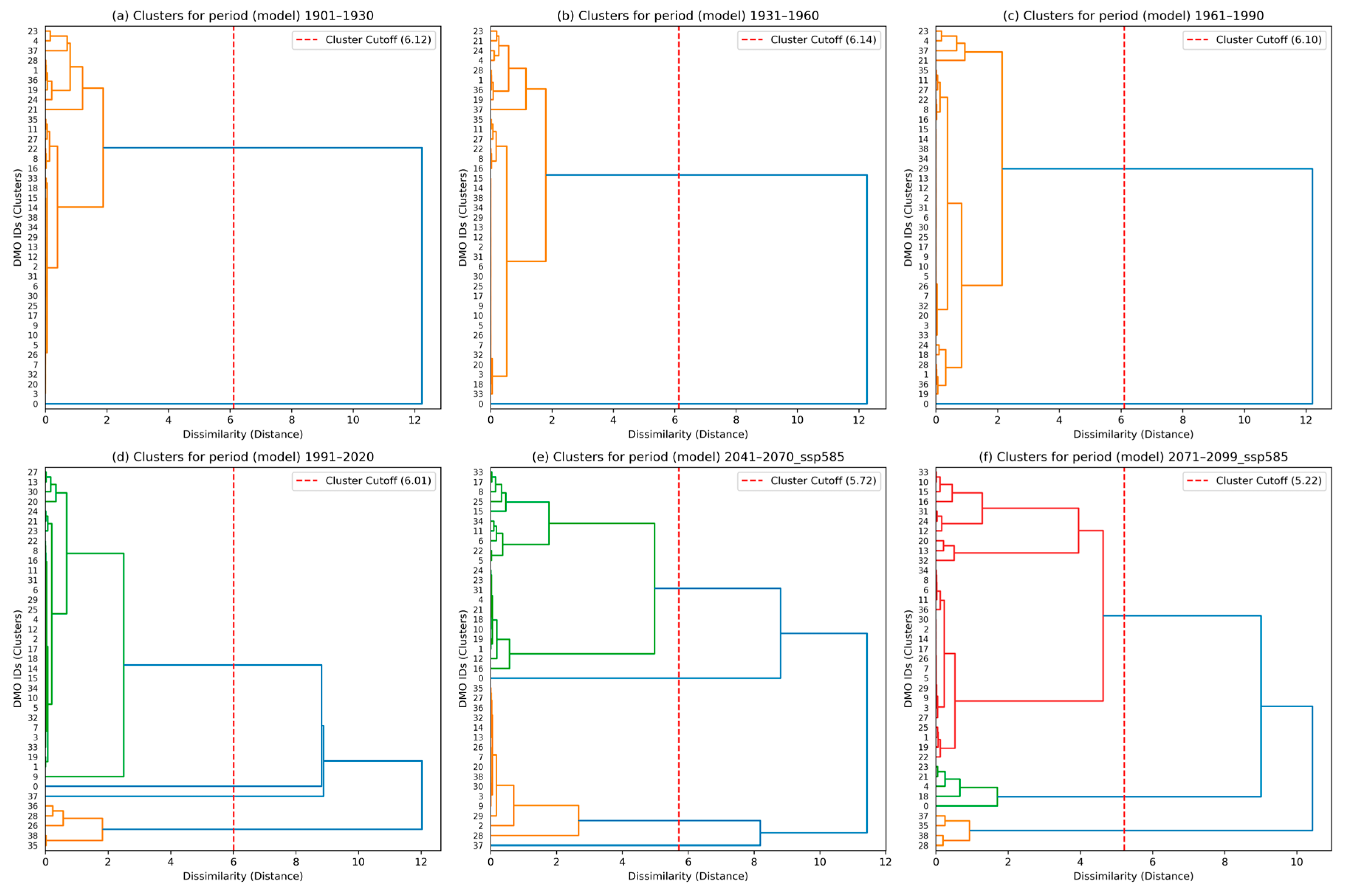
4.1. Clusters of DMOs by Köppen–Geiger Classification Main Groups

The similarity of the Köppen–Geiger classification main groups’ (hereinafter main climate) weight distribution indicates two clusters within the first three observed periods from 1901 to 1990 (Figure 2a–c). The first cluster consists of one individual DMO (DMO ID 1), and the second cluster contains the remaining DMOs. Both clusters in each period are represented by DMOs predominantly classified as Cold. A notable shift in the main climate differentiation arises in the fourth period, representing the years between 1991 and 2020 (Figure 2d). The first cluster remains; the second dissolves into three new clusters. One cluster contains an individual DMO (DMO ID 37), and one contains five DMOs (DMO IDs: 26, 28, 35, 36, and 38) that are no longer predominantly classified as Cold, but Temperate. The last cluster, representing all of the other DMOs, remains classified as Cold. In the fifth period, future projections for the years 2041–2071, a regrouping of two clusters is observable (Figure 2e). Of the two clusters containing only one DMO remain, one shifts to the Temperate climate zone. More importantly, the earlier smaller cluster of five DMOs grows by 11 members, indicating an increase in DMOs classified predominantly as Temperate. Within the last period, representing projections for 2071–2099, only three clusters remain (Figure 2f). The two clusters with one individual DMO regroup into two smaller clusters, one containing four DMOs (DMO IDs: 28, 35, 37, and 38) classified predominantly as Arid, and one containing five DMOs (Cluster 2 DMO IDs: 0, 4, 18, 21, and 23) classified as Cold, while the third cluster holds all of the other DMOs classified as Temperate.

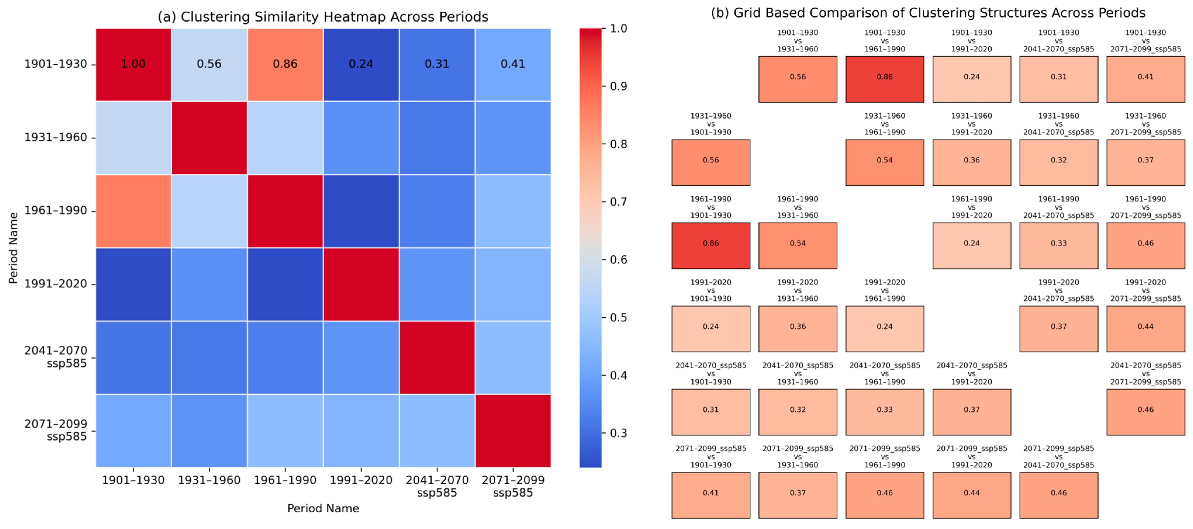
4.1.1. Clusters’ Structural Similarity

Comparing the clusters’ structural similarity over time (periods), most of the clusters shift moderately with a similarity correlation between 0.4 and 0.5 (Figure 3a,b); with the most extreme shift being observed between the periods 1960–1990 and 1991–2020 with a very low similarity correlation at 0.23, and subsequently between 1991–2020 and 2041–2071 with a score of 0.37 (Figure 3a,b). Notably, the period 1991–2020 is more similar to the latest future projection (2071–2099 with a similarity correlation of 0.46) than the first period (1901–1930 with a similarity correlation of 0.24). In other words, the current climate is less similar to the climate of our ancestors and more similar to the climate of our future descendants. Taking a closer look at the least similar periods, a proportionally stable distribution of weights among the DMOs may be observed in the 1960–1990 model, in contrast to a major shift in the clusters’ composition with larger mutual distances, indicating greater heterogeneity in the 1991–2020 model (Figure 2c,d).

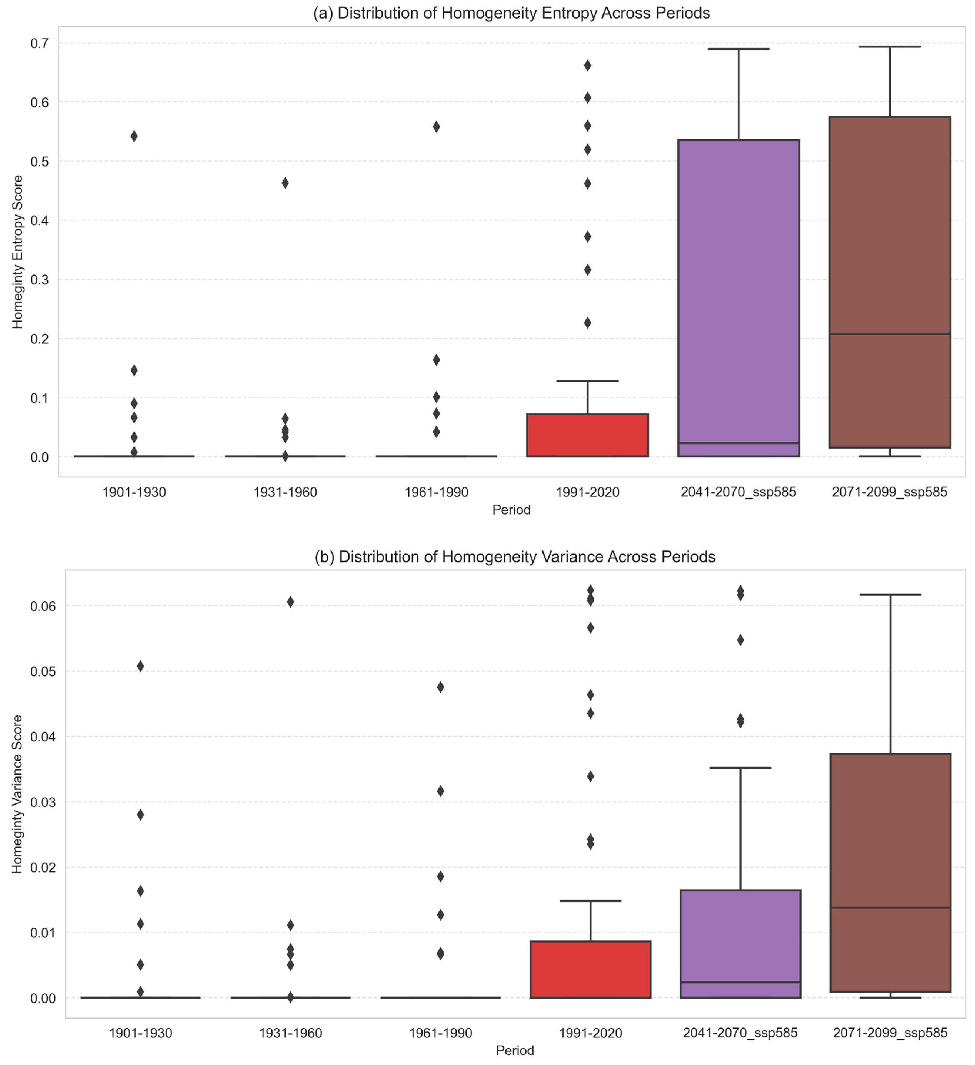
4.1.2. Change in Homogeneity Within the Köppen–Geiger Classification’s Main Climate

From the perspective of the main climate’s weight distribution uniformity across periods, the Shannon Entropy Analysis indicates shifts towards heterogeneity (Figure 4a). Within the first three observed periods, the majority of the DMOs recorded lower entropy scores, which indicates the dominant position of one main climate in a DMO, suggesting relatively stable homogeneity (Figure 4a). During the fourth period (1991–2020), the entropy scores begin to slightly grow; some DMOs (outliers with higher entropy) recorded a more even weight distribution of main climates and became more heterogeneous (Figure 4a). In the fifth period (2041–2070), the increase in heterogeneity is even more significant, observable through a higher median, wider range, and high outliers (Figure 4a). Compared to the previous periods, the last period (2071–2099) records the highest median entropy and a distribution leaning towards higher entropy scores, suggesting the lower homogeneity of the main climate categories within DMOs (Figure 4a).

Similarly, the Weighted Variance Analysis indicates very low fluctuations of the main climate categories’ weights in the first three periods (Figure 4b). The increase in variance and more fluctuation in some DMOs’ homogeneity may be observed in the fourth period (Figure 4b). The fourth and fifth periods record the highest fluctuation, the latter recording the most significant growth in variance, leading to an increase in the DMOs’ climate heterogeneity.

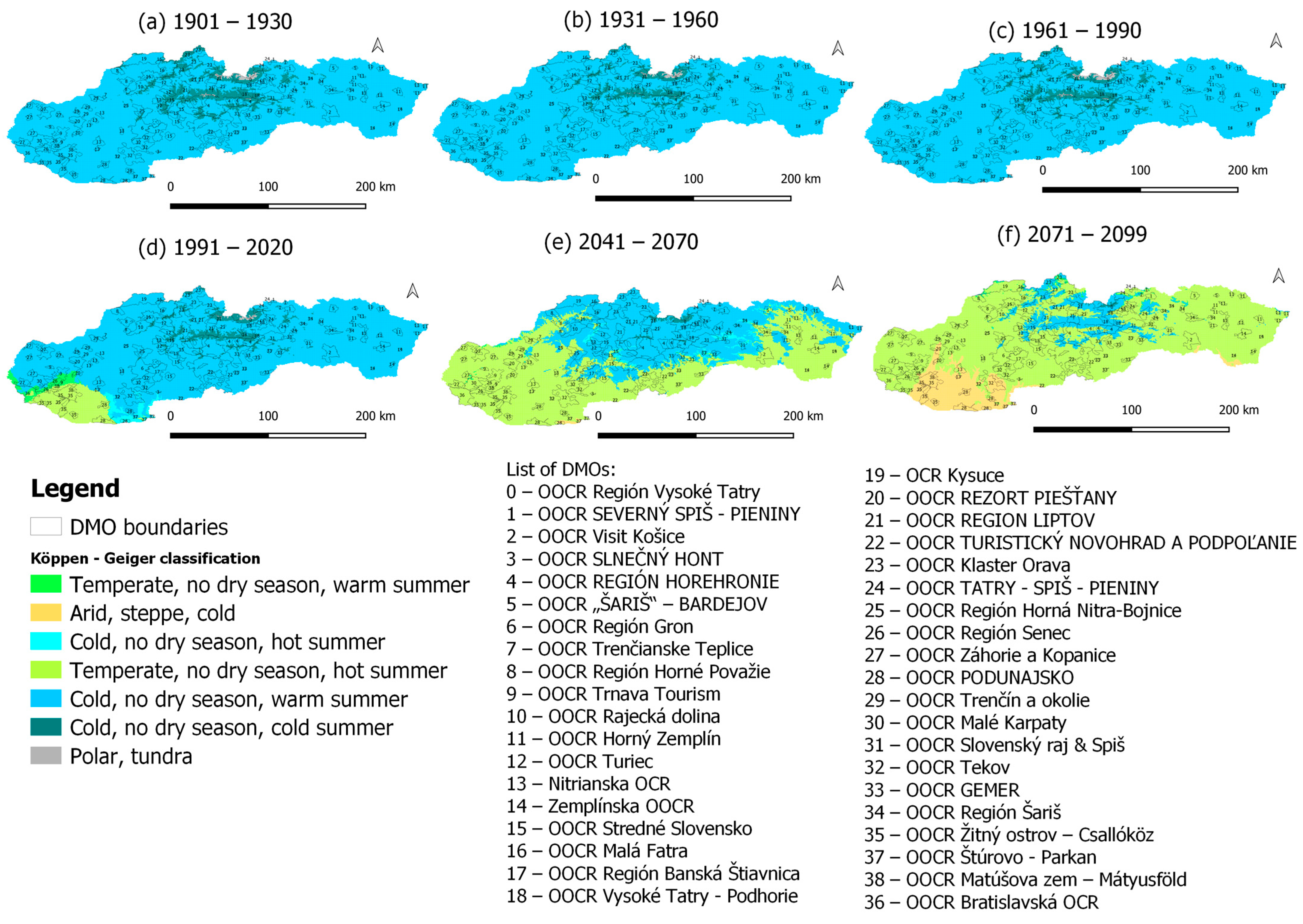
4.1.3. DMOs’ Main Climate Classification Changes

In terms of the main climate’s total weight change (total fluctuation), except for one (DMO ID 7), all of the DMOs experienced change (Figure 5a). In terms of both the median (0.98) and lower quartile (0.86), the observed changes are high (Figure 5a). A large majority of the DMOs (28) experienced extreme change (a weight change > 0.9), but the less changed DMOs still indicate quite significant changes between 0.55 and 0.87 (Figure 5a). Some of the DMOs (DMOs: 3, 9, 18, 21, 29) with extreme fluctuations indicate near-complete shifts in their main groups’ weight distributions (Figure 5a). Looking more closely at the descriptive statistics measured using the standard deviation, a variability between 0.43 and 0.47 may be observed for the highest fluctuations in 10 DMOs (4, 9, 13, 18, 19, 21, 23, 24, 27, and 29), which have the most unstable distributions in terms of their main climates’ weights (Figure 5b). Overall, the majority of the DMOs with a wide range of weights experienced significant shifts in the classifications of their main climates (Figure 5b).

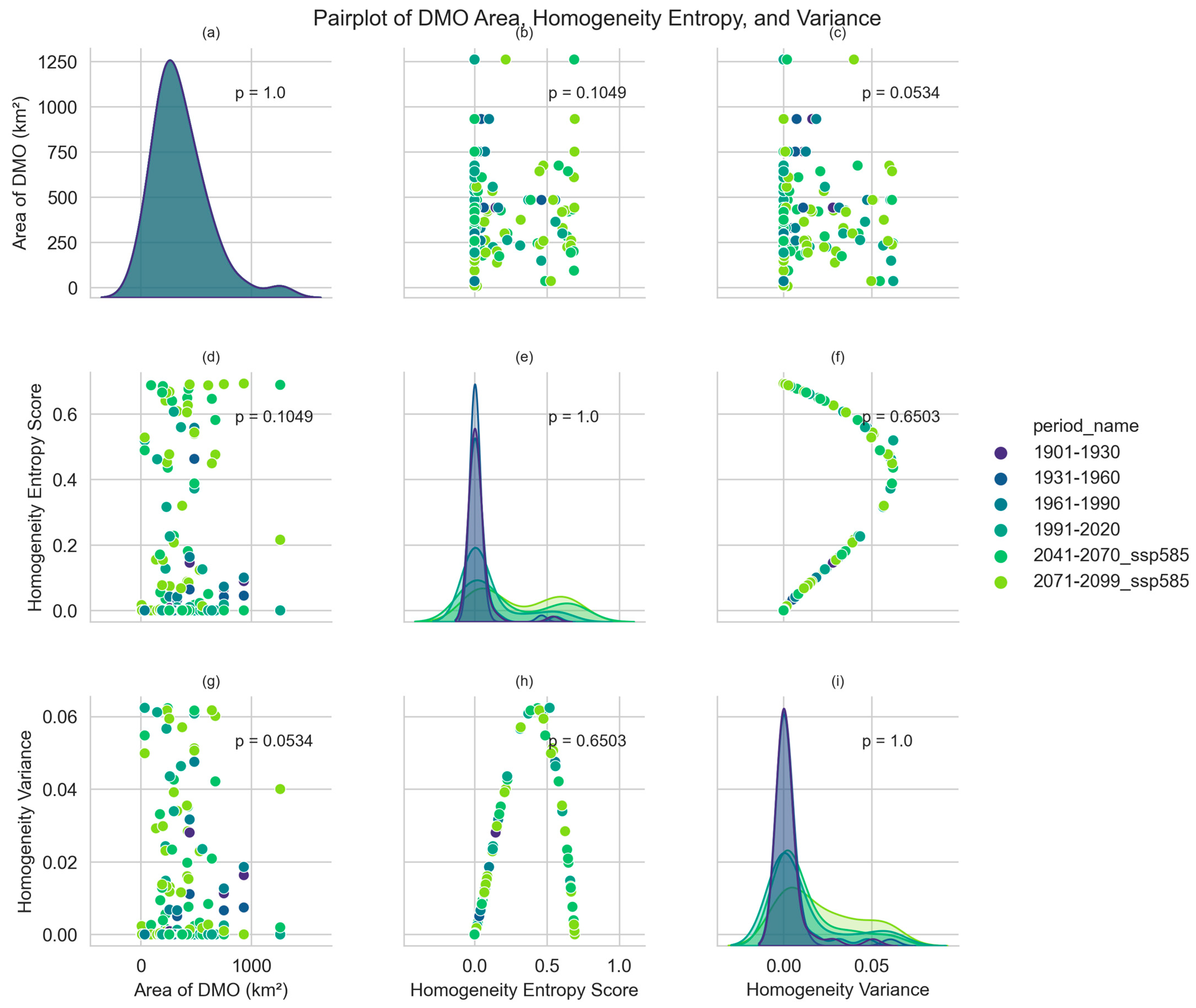
4.1.4. DMOs’ Area Size Relationship to Climate Homogeneity and Fluctuation

Even though the distribution of area sizes for the DMOs is positively skewed towards smaller areas (Figure 6a), only a very weak direct relationship is identified between the homogeneity of the DMOs’ main climates and their area sizes (Figure 6b,d). An even weaker correlation is indicated between DMOs’ area sizes and the main changes to their climates (Figure 6c,g). The low correlation values indicate no strong linearity between size and climate homogeneity or climate variance change. In other words, both smaller and larger destinations will be affected in the future, regardless of their area size.

In terms of main climate homogeneity, the Robust Regression Analysis results (coefficient = 2.78 × 10⁻⁵, p-value = 0.0049) indicate that the larger DMOs do tend to have an association with higher entropy and a more heterogenous distribution of main climates (Appendix A). From the perspective of the main climate fluctuations, the Robust Regression Analysis results (coefficient = 1.19 × 10⁻⁶, p-value = 0.055) indicate an association between area size and the increase in main climate variance change; however, only with a marginal statistical significance (Appendix A).

5. Discussion

The presented results reveal an evident transition in local DMOs from Cold to predominantly Temperate and, in some cases, even Arid climates, accompanied by increasing structural divergence, heterogeneity, and high fluctuation in the main climates’ composition. The identified patterns suggest gradual warming, as well as the fragmentation of local climate attributes, which will increasingly affect tourism-relevant natural resources. The results confirm that critical changes are already underway and are expected to intensify in the coming years, with significant implications for destination planning. As the timeline progresses toward the fifth projected period (2041–2070), the DMOs are expected to undergo significant changes in their dominant main climate class. Not only shifting toward warmer classifications but also exhibiting notable changes in climate homogeneity and variance.

The study contributes to the theoretical understanding of the relationships between climate change and tourism environment (destinations) by demonstrating how basic climate typologies can be monitored at a local scale via open data and statistical methods. In contrast to other resolutions (0.5 degrees and higher) that provide only generalized projections, the approach here allows for destination-specific analysis across time.

In relation to previous studies, the results are aligned with the urgent need for stakeholders to incorporate climate forecasting into local destinations’ decision-making processes in order to enhance resiliency (Scott et al. 2011; Gössling & Higham, 2020) [5,9]. The identified shift from Cold to Temperate climates, and even to an Arid climate, endorses the expectations of local seasonal tourism pattern change, similar to those identified by Carillo et al. (2022) [17]. The structural changes within the clusters, increasing heterogeneity and fluctuations in the main climate classes of the DMOs, support the significant transformation of tourism geographies (Hamilton et al., 2005; Ciscar et al., 2011) [15,16]. Following up on the role of DMOs as local facilitators in climate adaptation, as emphasized by Kaya (2025) and Rahman et al. (2025), more heterogeneous climates indicate that future strategies will have to be locally tailored and powered by big data running on both local stationary and remote sensing data [11,12]. Since climate change directly affects not only larger destinations but also smaller ones—without the necessary capacity, infrastructure, or financial resources—achieving climate resilience based on data-driven measures will be achievable only through stronger public–private–people collaborations, as pointed out by Scott et al. (2011) [14].

Additionally, the approach aligns with European and global climate governance frameworks, and the results reinforce the importance of integrating long-term climate data into tourism policy and capacity-building efforts. The presented approach’s results intend to support commitments in these frameworks, with emphasis on the criticality of integrating climate change considerations in DMOs’ processes. The future shifts in Slovak destinations’ main climates will change the current conditions of local landscapes and their vegetation, thus some of tourism’s natural resources may already be endangered, if not lost. Therefore, the results do confirm the criticality of protecting and restoring the local ecosystem contained in the Glasgow Declaration’s Regenerate pathway (One Planet Sustainable Tourism Programme, 2021) [2]. While the Köppen–Geiger classification does not communicate the dangers of GHG emissions, the classification’s data clearly express environmental impact at the local destination level. Subjectively, the communication of identified shifts may support local DMOs’ role in starting capacity-building and education contained in the UNWTO’s policy guidance or in the European Agenda (European Union, 2022; UNWTO, 2024) [3,4].

From a practical perspective, the results support the development of tailored climate adaptation strategies by DMOs and offer a globally reproducible approach. By grouping destinations into clusters, the study provides a framework for peer learning among similarly affected areas. If extended to other countries, it could also support cross-border knowledge exchange. In support of DMOs’ role in climate education and information dissemination, the resulting public dashboard can be utilized by any local DMO or tourism stakeholder [7,8,31]. Each DMO can be examined individually within its defined territorial boundaries across the available periods [29]. From a managerial perspective, although each DMO will need to respond to these changes independently, their positioning within shared climate clusters offers opportunities to exchange best practices and collaborate on adaptation strategies, thereby strengthening collective advocacy efforts and potentially motivating government authorities to allocate targeted funding for climate resilience actions within Slovak destinations.

Despite its contributions, this study has its limitations within the extent of the analyzed indicators and the granularity of the input data. Firstly, while the Köppen–Geiger classification projections are easily accessible, and should be understandable to ordinary citizens, the classification has its limits, mainly in terms of its nature of communicating information derived from aggregated temperature, humidity, and, in some versions, altitude data.

Secondly, due to the restricted interpretation of the findings to broader climate trends, the approach must be extended in the future to capture related behavioral dimensions and economic impacts. To deliver more complex information for local DMOs and stakeholders, the current study will be extended with indicators focusing on tourists’ comfort (e.g., the Tourism Climate Index, Holiday Climate Index, and Summer Simmer Index) and safety (e.g., Air Quality, GHG emissions, and CO₂ concentrations). To raise awareness and motivate local transition to climate resilience, future research will have to utilize open satellite imagery techniques for natural and cultural heritage vulnerability (e.g., NDVI).

Last but not least, although the approach simplifies access to climate data, it still assumes a baseline of willingness to learn and the level of digital capacity within DMOs, which may vary significantly. Due to this, additional research is needed to assess how different DMOs can realistically utilize climate change data.

References

1. United Nations. Paris Agreement. United Nations Framework Convention on Climate Change, 2015. Available online: https://unfccc.int/sites/default/files/english_paris_agreement.pdf (accessed on 1 January 2025).
2. One Planet Sustainable Tourism Programme. Glasgow Declaration: A Commitment to a Decade of Climate Action. 2021. Available online: https://www.oneplanetnetwork.org/sites/default/files/2022-02/GlasgowDeclaration_EN_0.pdf (accessed on 1 January 2025).
3. World Tourism Organization. Policy Guidance to Support Climate Action by National Tourism Administrations; UN Tourism: Madrid, Spain, 2024. [Google Scholar] [CrossRef]
4. Council of the European Union. European Agenda for Tourism 2030—Council Conclusions (Adopted on 01/12/2022); General Secretariat of the Council: Brussel, Belgique, 2022; Available online: https://data.consilium.europa.eu/doc/document/ST-15441-2022-INIT/en/pdf (accessed on 1 January 2025).
5. Scott, D.; Amelung, B.; Becken, S.; Ceron, J.P.; Dubois, G.; Gössling, S.; Peeters, P.; Simpson, M.C. Climate Change and Tourism: Responding to Global Challenges; World Tourism Organization (UNWTO): Madrid, Spain; United Nations Environment Programme (UNEP): Nairobi, Kenya, 2008. [Google Scholar]
6. Dodds, R. Destination marketing organizations and climate change: The need for leadership and education. Sustainability 2010, 2, 3449–3464. [Google Scholar] [CrossRef]
7. Bhandari, K.; Cooper, C.P.; Ruhanen, L. The Role of the Destination Management Organisation in Responding to Climate Change: Organisational Knowledge and Learning. Acta Tur. 2014, 26, 91–102. [Google Scholar]
8. Bhandari, K.; Cooper, C.; Ruhanen, L. Climate change knowledge and organizational adaptation: A destination management organization case study. Tour. Recreat. Res. 2015, 41, 60–68. [Google Scholar] [CrossRef]
9. Gössling, S.; Higham, J. The low-carbon imperative: Destination management under urgent climate change. J. Travel Res. 2020, 59, 581–598. [Google Scholar] [CrossRef]
10. MacEachern, J.; MacInnis, B.; MacLeod, D.; Munkres, R.; Jaspal, S.K.; Kinay, P.; Wang, X. Destination Management Organizations’ Roles in Sustainable Tourism in the Face of Climate Change: An Overview of Prince Edward Island. Sustainability 2024, 16, 3049. [Google Scholar] [CrossRef]
11. Kaaya, N.D. The Role of Networks Among Destination Management Organizations in Promoting Destinations’ Sustainability and Resilience: A Mixed-Methods Study. Doctoral Dissertation, University of South-Eastern Norway, Notodden, Norway, 2025. [Google Scholar]
12. Rahman, T.U.; Saud, D.; Nawaz, T. Sustainable tourism in a changing climate: Strategies for management, adaptation, and resilience. Int. J. Sustain. Tour. 2024, 1, e-24001. Available online: https://journals.penrosehub.org/index.php/home/article/view/13 (accessed on 1 January 2025). [CrossRef]
13. d’Angella, F.; Maccioni, F.; De Carlo, M. Exploring destination sustainable development strategies: Triggers and levels of maturity. Sustain. Futures 2025, 9, 100515. [Google Scholar] [CrossRef]
14. Scott, D.; Lemieux, C.J.; Malone, L. Climate services to support sustainable tourism development and adaptation to climate change. Clim. Res. 2011, 47, 111–122. [Google Scholar] [CrossRef]
15. Hamilton, J.M.; Maddison, D.J.; Tol, R.S.J. The effects of climate change on international tourism. Clim. Res. 2005, 29, 245–254. [Google Scholar] [CrossRef]
16. Ciscar, J.-C.; Iglesias, A.; Feyen, L.; Szabó, L.; Van Regemorter, D.; Amelung, B.; Nicholls, R.; Watkiss, P.; Christensen, O.B.; Dankers, R.; et al. Physical and economic consequences of climate change in Europe. Proc. Natl. Acad. Sci. USA 2011, 108, 2678–2683. [Google Scholar] [CrossRef]
17. Carrillo, J.; González, A.; Pérez, J.C.; Expósito, F.J.; Díaz, J.P. Projected impacts of climate change on tourism in the Canary Islands. Reg. Environ. Change 2022, 22, 61. [Google Scholar] [CrossRef]
18. Farooq, M.A.; Ghufran, M.A.; Ahmed, N.; Attia, K.A.; Mohammed, A.A.; Hafeez, Y.M.; Amanat, A.; Farooq, M.S.; Uzair, M.; Naz, S. Remote sensing analysis of spatiotemporal impacts of anthropogenic influence on mountain landscape ecology in Pir Chinasi National Park. Sci. Rep. 2024, 14, 20695. [Google Scholar] [CrossRef]
19. Boori, M.S.; Choudhary, P.; Kučera, F. Land use/cover disturbance due to tourism in Jeseníky Mountain, Czech Republic: A remote sensing and GIS-based approach. Environ. Earth Sci. 2015, 74, 997–1006. [Google Scholar] [CrossRef]
20. Helali, J.; Asaadi, S.; Jafarie, T.; Habibi, M.; Salimi, S.; Momenpour, S.E.; Shahmoradi, S.; Hosseini, S.A.; Hessari, B.; Saeidi, V. Drought monitoring and its effects on vegetation and water extent changes using remote sensing data in Urmia Lake watershed, Iran. J. Water Clim. Change 2022, 13, 2107–2128. [Google Scholar] [CrossRef]
21. Xue, Z.; Chen, L.; Gong, J.; Shen, S. Assessing the impact of climate change on tourism climate resources using high-resolution remote sensing data. Remote Sens. 2022, 14, 2857. [Google Scholar] [CrossRef]
22. Zhang, Y.; Wang, L.; Zhou, L. Future risk of tourism pressures under climate change: A remote sensing approach. Remote Sens. 2022, 14, 3758. [Google Scholar] [CrossRef]
23. García, D.H.; Rezapouraghdam, H.; Hall, C.M.; Karatepe, O.M.; Koupaei, S.N. Spatio-temporal variability of the earth’s surface temperature and the changes in land use/land cover: Implications for sustainable tourism development. J. Sustain. Tour. 2023, 17, 557–584. [Google Scholar] [CrossRef]
24. Köppen, W. Klassification der Klimate nach Temperatur, Niederschlag and Jahreslauf. In Petermanns Geographische Mitteilungen; Gotha: Hamburg, Germany, 1918; Volume 64, pp. 193–203, 243–248. Available online: https://koeppen-geiger.vu-wien.ac.at/pdf/Koppen_1918.pdf (accessed on 1 January 2025).
25. Geiger, R. Klassifikation der Klimate nach W. Köppen. In Landolt-Börnstein—Zahlenwerte und Funktionen aus Physik, Chemie, Astronomie, Geophysik und Technik, Alte Serie; Springer: Berlin/Heidelberg, Germany, 1954; Volume 3, pp. 603–607. [Google Scholar]
26. Peel, M.C.; Finlayson, B.L.; McMahon, T.A. Updated world map of the Köppen-Geiger climate classification. Hydrol. Earth Syst. Sci. 2007, 11, 1633–1644. [Google Scholar] [CrossRef]
27. Beck, H.E.; Zimmermann, N.E.; McVicar, T.R.; Vergopolan, N.; Berg, A.; Wood, E.F. Present and future Köppen-Geiger climate classification maps at 1-km resolution. Sci. Data 2018, 5, 180214. [Google Scholar] [CrossRef]
28. Beck, H.E.; McVicar, T.R.; Vergopolan, N.; Berg, A.; Lutsko, N.J.; Dufour, A.; Zeng, Z.; Jiang, X.; van Dijk, A.I.J.M.; Miralles, D. High-resolution (1 km) Köppen-Geiger maps for 1901–2099 based on constrained CMIP6 projections. Sci. Data 2023, 10, 724. [Google Scholar] [CrossRef]
29. Sidor, C. SK DMOs Territory Köppen-Geiger Climate Classification. Github. 2025. Available online: https://github.com/csabasidor/SK-DMOs-territory---Koppen-Geiger-climate-classification-/tree/main (accessed on 1 January 2025).
30. Sidor, C. get_dmo_base_data.py. SK-Geoheritage-at-TripAdvisor. Github. 2024. Available online: https://github.com/csabasidor/SK-Geoheritage-at-TripAdvisor/blob/main/source_codes/modules/get_dmo_base_data.py (accessed on 1 January 2025).
31. Sidor, C. SK DMOs Change of Köppen-Geiger Climate Classification (1901–2099). 2025. Available online: https://cases.idoaba.eu/sk_dmos_kgc/ (accessed on 1 January 2025).
32. Pedregosa, F.; Varoquaux, G.; Gramfort, A.; Michel, V.; Thirion, B.; Grisel, O.; Blondel, M.; Prettenhofer, P.; Weiss, R.; Dubourg, V.; et al. Scikit-learn: Machine learning in Python. J. Mach. Learn. Res. 2011, 12, 2825–2830. Available online: https://jmlr.org/papers/v12/pedregosa11a.html (accessed on 1 January 2025).
33. Virtanen, P.; Gommers, R.; Oliphant, T.E.; Haberland, M.; Reddy, T.; Cournapeau, D.; Burovski, E.; Peterson, P.; Weckesser, W.; Bright, J.; et al. SciPy 1.0: Fundamental algorithms for scientific computing in Python. Nat. Methods 2020, 17, 261–272. [Google Scholar] [CrossRef] [PubMed]
34. Ward, J.H. Hierarchical grouping to optimize an objective function. J. Am. Stat. Assoc. 1963, 58, 236–244. [Google Scholar] [CrossRef]
35. Press, W.H.; Teukolsky, S.A.; Vetterling, W.T.; Flannery, B.P. Numerical Recipes: The Art of Scientific Computing, 3rd ed.; Cambridge University Press: Cambridge, UK, 2007. [Google Scholar]
36. Pearson, K. Note on regression and inheritance in the case of two parents. Proc. R. Soc. Lond. 1895, 58, 240–242. [Google Scholar] [CrossRef]
37. Shannon, C.E. A mathematical theory of communication. Bell Syst. Tech. J. 1948, 27, 379–423. [Google Scholar] [CrossRef]
38. Hastie, T.; Tibshirani, R.; Friedman, J. The Elements of Statistical Learning: Data Mining, Inference, and Prediction, 2nd ed.; Springer: Berlin/Heidelberg, Germany, 2009. [Google Scholar] [CrossRef]
39. Seabold, S.; Perktold, J. Statsmodels: Econometric and statistical modeling with Python. In Proceedings of the 9th Python in Science Conference, Austin, TX, USA, 28–30 June 2010; pp. 92–96. [Google Scholar]
40. Huber, P.J. Robust estimation of a location parameter. Ann. Math. Stat. 1964, 35, 73–101. [Google Scholar] [CrossRef]
Figure 1. Köppen–Geiger climate classification maps of Slovakia in relation to DMO boundaries across periods. (a) 1901–1930; (b) 1931–1960; (c) 1960–1990; (d) 1991–2020; (e) 2041–2070 (version ssp585); (f) 2071–2099 (version ssp585).
World 06 00068 g001
Figure 2. DMO clusters by weights of the Köppen–Geiger classification’s main climate across periods (cluster colors based on cutoff distance threshold). (a) 1901–1930; (b) 1931–1960; (c) 1960–1990; (d) 1991–2020; (e) 2041–2070 (version ssp585); and (f) 2071–2099 (version ssp585).
World 06 00068 g002
Figure 3. Periodwise Clustering Comparison of Köppen–Geiger classification’s main group. (a) Clustering heatmap of similarity correlation; (b) grid-based comparison of periods’ similarity correlation.
World 06 00068 g003
Figure 4. Distribution of DMOs’ climate homogeneity across periods. (a) Entropy; (b) variance.
World 06 00068 g004
Figure 5. DMOs’ main climate classification change. (a) Range of weight changes; (b) distribution of weight changes.
World 06 00068 g005
Figure 6. Direct linear relationships of DMOs’ area sizes, homogeneity entropy, and variance. (a) Kernel Density Estimation for distribution of DMOs’ area; (b) Correlation test for DMOs’ area vs. Homogeneity Entropy Score; (c) Correlation test for DMOs’ area vs. Homogeneity Variance; (d) Correlation test for Homogeneity Entropy Score vs. DMOs’ area; (e) Kernel Density Estimation for distribution of Homogeneity Entropy Score; (f) Correlation Test for Homogeneity Entropy Score vs. Homogeneity Variance; (g) Correlation Test for Homogeneity Variance vs. DMO area; (h) Correlation Test Homogeneity Variance vs. Homogeneity Entropy Score; (i) Kernel Density Estimation for distribution of Homogeneity Variance.
World 06 00068 g006
Disclaimer/Publisher’s Note: The statements, opinions and data contained in all publications are solely those of the individual author(s) and contributor(s) and not of MDPI and/or the editor(s). MDPI and/or the editor(s) disclaim responsibility for any injury to people or property resulting from any ideas, methods, instructions or products referred to in the content.